7

Epidemiological studies

JULIE A MORRIS, MARTIN J GARDNER

The techniques for obtaining confidence intervals for estimates of relative risks, attributable risks and odds ratios are described. These can come either from an incidence study, where, for example, the frequency of a congenital malformation at birth is compared in two defined groups of mothers, or from a case-control study, where a group of patients with the disease of interest (the cases) is compared with another group of people without the disease (the controls).

The methods of obtaining confidence intervals for standardised disease ratios and rates in studies of incidence, prevalence, and mortality are described. Such rates and ratios are commonly calculated to enable appropriate comparisons to be made between study groups after adjustment for confounding factors like age and sex. The most frequently used standardised indices are the standardised incidence ratio (SIR) and the standardised mortality ratio (SMR).

Some of the methods given here are large sample approximations but will give reasonable estimates for small studies. Appropriate design principles for these types of study have to be adhered to, since confidence intervals convey only the effects of sampling variation on the precision of the estimated statistics. They cannot control for other errors such as biases due to the selection of inappropriate controls or in the methods of collecting the data.

Relative risks, attributable risks and odds ratios

Incidence study

Suppose that the incidence or frequency of some outcome is assessed in two groups of individuals defined by the presence or absence of some characteristic. The data from such a study can be presented as in Table 7.1.

Table 7.1 Classification of outcome by group characteristic

The outcome probabilities in exposed and unexposed individuals are estimated from the study groups by A/(A + C) and B/(B + D) respectively. An estimate, R, of the relative risk (or risk ratio) from exposure is given by the ratio of these proportions, so that

Confidence intervals for the population value of R can be constructed through a logarithmic transformation.¹ The standard error of log_e R is

This can also be written as

A 100(1 – α)% confidence interval for R is found by first calculating the two quantities

and

where Z_{1 – α/2} is the appropriate value from the standard Normal distribution for the 100(1 – α/2) percentile found in Table 18.1. The confidence interval for the population value of R is then given by exponentiating W and X as

Table 7.2 Prevalence of Helicobacter pylori infection in preschool children according to mother’s history of ulcer²

Worked example

Brenner et al. reported the prevalence of Helicobacter pylori infection in preschool children according to parental history of duodenal or gastric ulcer.² The results are shown in Table 7.2.

An estimate of the relative risk of Helicobacter pylori infection associated with a history of ulcer in the mother is

The standard error of log_e R is

from which for a 95% confidence interval

and

The 95% confidence interval for the population value of R is then given as that is, from 1·01 to 4·14. The estimated risk of Helicobacter pylori infection in children with a history of ulcer in the mother is 205% of that in children without a history of ulcer in the mother with a 95% confidence interval of 101% to 414%.

A measure of the proportion of individuals in the total population with the disease attributed to exposure to the risk factor is given by the attributable risk (AR). If p is the prevalence of the risk factor in the population and R is the relative risk for disease associated with the risk factor, then

If the prevalence, p, is assumed to have negligible sampling variation, then the 100(1 – α)% confidence interval for AR can be derived by obtaining confidence limits for the relative risk, R, as described previously and substituting these into the formula for AR given above.³ (See chapter 13 for discussion of this ‘substitution’ method.) This approach will give a reasonable approximation to confidence intervals derived from a more exact method. It is important to note that this method is not appropriate for substitution of a confounder-adjusted relative risk.^{4, 5}

Denoting the confidence interval for R by R_L to R_U, the 100(1 – α)% confidence interval for AR is given by

Worked example

In the previous example, the prevalence of history of ulcer in mothers of preschool children is 22/863 = 0·0255, and the relative risk of Helicobacterpylori infection associated with a history of ulcer is 2·05.² An estimate of the attributable risk is

As already calculated, the 95% confidence interval for R is given by R_L = 1·01 to R_U = 4·14. The 95% confidence interval for AR is thus

that is, from 0·0003 to 0·0741. The proportion of children with Helicobacter pylori infection due to history of ulcer in the mother is estimated at 26 per 1000 with a wide 95% confidence interval ranging from 0·3 per 1000 to 74 per 1000.

Unmatched case-control study

Suppose that groups of cases and controls are studied to assess exposure to a suspected causal factor. The data can be presented as in Table 7.3.

An approximate estimate of the relative risk for the disease associated with exposure to the factor can be obtained from a case-control study through the odds ratio,⁶ the relative risk itself not being directly estimable with this study design. The odds ratio (OR) is given as

Table 7.3 Classification of exposure among cases and controls

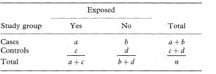
A confidence interval for the population odds ratio can be constructed using several methods which vary in their ease and accuracy. The method described here (sometimes called the logit method) was devised by Woolf⁷ and is widely recommended as a satisfactory approximation. The exception to this is when any of the numbers a, b, c, or d is small, when a more accurate but complex procedure should be used if suitable computer facilities are available. Further discussion and comparison of methods can be found in Breslow and Day.⁸ The use of the following approach, however, should not in general lead to any misinterpretation of the results.

The logit method uses the Normal approximation to the distribution of the logarithm of the odds ratio (log_e OR) in which the standard error is

A 100(1 – α)% confidence interval for OR is found by first calculating the two quantities

and

where z_{1 – α/2} is the appropriate value from the standard Normal distribution for the 100(1 – α/2) percentile (see Table 18.1). The confidence interval for the odds ratio in the population is then obtained by exponentiating Y and Z to give

Worked example

ABO non-secretor state was determined for 114 patients with spondyloarthropathies and 334 controls⁹ with the results shown in Table 7.4.

Table 7.4 ABO non-secretor state for 114 patients with spondyloarthropathies and 334 controls⁹

The estimated odds ratio for spondyloarthropathies with ABO non-secretor state is OR = (54 × 245)/(60 × 89) = 2·48. The standard error of log_e OR is

For a 95% confidence interval

and

The 95% confidence interval for the population value of the odds ratio for spondyloarthropathies with ABO non-secretor state is then given as

that is, from 1·59 to 3·85. These results show that the estimated risk of spondyloarthropathy with ABO non-secretor state is 248% of that without ABO non-secretor state with 95% confidence interval of 159% to 385%.

More than two levels of exposure

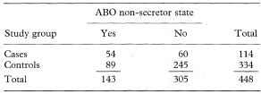
If there are more than two levels of exposure, one can be chosen as a baseline with which each of the others is compared. Odds ratios and their associated confidence intervals are then calculated for each comparison in the same way as shown previously for only two levels of exposure.

A series of unmatched case-control studies

A combined estimate is sometimes required when independent estimates of the same odds ratio are available from each of K sets of data—for example, in a stratified analysis to control for confounding variables.

One approach is to use the logit method to give a pooled estimate of the odds ratio (OR_logit) and then derive a confidence interval for the odds ratio in a similar way to that for a single 2 × 2 table. The logit combined estimate (OR_logit) is defined by

where OR_i = a_id_i/b_ic_i is the odds ratio in the ith table, a_i, b_i, c_i, and d_i are the frequencies in the ith 2 × 2 table, n_i = a_i + b_i + c_i + d_i, the summation ∑ is over i = 1 to K for the K tables and w_i is defined as

The standard error of log_e (OR_logit) is given by

where w = ∑w_i.

A 100(1 – α)% confidence interval for OR_logit can then be found by calculating

and

where z_{1 – α/2} is the appropriate value from the standard Normal distribution for the 100(1 – α/2) percentile (see Table 18.1).

The confidence interval for the population value of OR_logit is given by exponentiating U and V as

It is important to mention that, before combining independent estimates, there should be some reassurance that the separate odds ratios do not vary markedly, apart from sampling error.^6,8 Hence, a test for homogeneity of the odds ratio over the strata is recommended. Further discussion of homogeneity tests, methods for the calculation of 95% confidence intervals and a worked example are given in Breslow and Day.⁸ The logit method is unsuitable if any of the numbers a_i, b_i, c_i or d_i is small. This will happen, for example, with increasing stratification, and in such cases a more complex exact method is available.⁸

An alternative approach which gives a consistent estimate of the common odds ratio with large numbers of small strata is to use the Mantel–Haenszel pooled estimate of the odds ratio (OR_{M – H}) which is given by

A method of calculating confidence intervals for this estimate is described in Armitage and Berry.⁶ It is more complex, however, than the previous approach which extends the single case-control technique shown earlier. For samples of reasonable size both methods will usually give similar values for the combined odds ratio and confidence interval.

The scope of a stratified analysis for case-control studies can be extended using a logistic regression model.⁸ This also enables the joint effects of two or more factors on disease risk to be assessed (see chapter 8).

Worked example

A number of studies examining the relationship of passive smoking exposure to lung cancer were reviewed by Wald et al.¹⁰ The findings, which are shown in Table 7.5, included those from four studies of women in the USA. They are used below to illustrate the combination of results from independent sets of data. A test for homogeneity of the odds ratio provided no evidence of a difference between the four studies.

The logit combined estimate of the odds ratio (OR_logit) over the four studies is found to be 1·19. The standard error of log_e (OR_logit) is 0·1694.

For a 95% confidence interval

and

Table 7.5 Exposure to passive smoking among female lung cancer cases and controls in four studies¹⁰

The 95% confidence interval for the population value of the odds ratio of lung cancer associated with passive smoking exposure is then given by

that is, from 0·85 to 1·66. The risk of lung cancer with passive smoking exposure is estimated to be 119% of that with no passive smoking exposure with a 95% confidence interval of 85% to 166%.

If, alternatively, the Mantel–Haenszel method is used on these data the combined estimate of the odds ratio is found to be also 1·19, with a 95% confidence interval of 0·86 to 1·66, virtually the same result.

Matched case-control study

If each of n cases of a disease is matched to one control to form n pairs and each individual’s exposure to a suspected causal factor is recorded the data can be presented as in Table 7.6. For this type of study an approximate estimate (in fact the Mantel–Haenszel estimate) of the relative risk of the disease associated with exposure is again given by the odds ratio which is now calculated as

An exact 100(1 – α)% confidence interval for the population value of OR is found by first determining a confidence interval for s (the number of case-control pairs with only the case exposed).⁶ Conditional on the sum of the numbers of “discordant” pairs (s + t) the number s can be considered as a Binomial variable with sample size s + t and proportion s/(s + t).

The 100(1 – α)% confidence interval for the population value of the Binomial proportion can be obtained from tables based on the Binomial distribution (for example, Lentner¹¹). If this confidence interval is denoted by A_L to A_U the 100(1 – α)% confidence interval for the population value of OR is then given by

Table 7.6 Classification of matched case-control pairs by exposure

Worked example

Thirty-five patients who died in hospital from asthma were individually matched for sex and age with 35 control subjects who had been discharged from the same hospital in the preceding year.¹² The inadequacy of monitoring of all patients while in hospital was independently assessed; the paired results are given in Table 7.7.

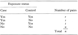
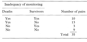
Table 7.7 Inadequacy of monitoring in hospital of deaths and survivors among 35 matched pairs of asthma patients¹²

The estimated odds ratio of dying in hospital associated with inadequate monitoring is OR = 13/3 = 4·33.

From the appropriate table for the Binomial distribution with sample size s + t = 13 + 3 = 16, proportion s/(s + t) = 13/(13 + 3) = 0·81, and α = 0·05, the 95% confidence interval for the population value of the Binomial proportion is found to be A_L = 0·5435 to A_U = 0·9595. The 95% confidence interval for the population value of the odds ratio is thus

that is, from 1·19 to 23·69. The risk of dying in hospital following inadequate monitoring is estimated to be 433% of that with adequate monitoring, with a very wide 95% confidence interval ranging from 119% to 2369%, reflecting the imprecision in this estimate.

Matched case-control study with 1: M matching

Sometimes each case is matched with more than one control. The odds ratio is then given by the Mantel–Haenszel estimate as

where M is the number of matched controls for each case, is the number of matched sets in which the case and i – 1 of the matched controls are exposed, n_i⁽⁰⁾ is the number of sets in which the case is unexposed and i of the matched controls are exposed, and the summation is from i = 1 to M.

A confidence interval for the population value of OR_{M – H} can be derived by one of the methods in Breslow and Day.⁸ These authors also explain the calculation of a confidence interval for the odds ratio estimated from a study with a variable number of matched controls for each case.⁸

Incidence rates, standardised ratios and rates

Incidence rates

If x is the observed number of individuals with the outcome (or disease) of interest, and Py the number of person-years at risk, the incidence rate is given by IR = x/Py.

The 100(1 – α)% confidence interval for the population value of IR can be calculated by first assuming x to have a Poisson distribution, and finding its related confidence interval.³ Table 18.3 gives 90%, 95% and 99% confidence intervals for x in the range 0 to 100. It also indicates how to obtain approximate confidence intervals for x taking values greater than 100. Denote this confidence interval by x_L to x_U. Assuming Py is a constant with no sampling variation, the 100(1 – α)% confidence interval for IR is given by

Worked example

Nunn et al. published mortality figures for the period 1990–95 in a rural population in south-west Uganda.¹³ They reported 28 deaths among children aged 5–12 years over 10992 person-years of observation.

Taking x = 28 and Py = 10 992, the death rate for 5–12-year olds is IR = 28/10 992 = 2·55. deaths per 1000 person-years. The 95% confidence limits for the number of deaths, x_L = 18·6 and x_U = 40·5 are found from Table 18.3 with x = 28 and α = 0·05.

The 95% confidence interval for the death rate is

that is, from 1·69 to 3·68 per 1000 person-years.

Standardised ratios

If O is the observed number of incident cases (or deaths) in a study group and E the expected number based on, for example, the age-specific disease incidence (or mortality) rates in a reference or standard population the standardised incidence ratio (SIR) or standardised mortality ratio (SMR) is O/E. This is usually called the indirect method of standardisation because the specific rates of a standard population are used in the calculation rather than the rates of the study population. The expected number is calculated as

where n_i is the number of individuals in age group i of the study group, DR_i is the death rate in age group i of the reference population, and ∑ denotes summation over all age groups.

The 100(1 – α)% confidence interval for the population value of O/E can be found by first regarding O as a Poisson variable and finding its related confidence interval¹⁴ (see Table 18.3). Denote this confidence interval by O_L to O_U.

The 100(1 – α)% confidence interval for the population value of O/E is then given by

Worked example

Roman et al. observed 64 cases of leukaemia in children under the age of 15 years in the West Berkshire Health Authority area during 1972–85.¹⁵ They calculated that 45·6 cases would be expected in the area at the age specific leukaemia registration rates by calendar year for this period in England and Wales (the standard population). Using O = 64 and E = 45·6 the standardised incidence ratio (SIR) is 64/45·6 = 1·40. Values of O_L = 49·3 and O_U = 81·7 are found from the appropriate table based on the Poisson distribution when O = 64 and α = 0·05 (see Table 18.3).

The 95% confidence interval for the population value of the standardised incidence ratio is

that is, from 1·08 to 1·79. The uncertainty in the incidence rate in West Berkshire ranges from just 8% greater incidence to almost 80% greater incidence compared to the standard England and Wales population.

Sometimes the standardised incidence ratio (or standardised mortality ratio) is multiplied by 100 and then the same must be done to the figures describing the confidence interval.

Ratio of two standardised ratios

Let O₁ and O₂ be the observed numbers of cases (deaths) in two study groups and E₁ and E₂ the two expected numbers. It is sometimes appropriate to calculate the ratio of the two standardised incidence ratios (standardised mortality ratios) O₁/E₁ and O₂/E₂ and find a confidence interval for this ratio. Although there are known limitations to this procedure if the age-specific incidence ratios within each group to the standard are not similar, these are not serious in usual applications.¹⁴ Again O₁ and O₂ can be regarded as Poisson variables and a confidence interval for the ratio O₁/O₂ is obtained as described by Ederer and Mantel.¹⁶ The procedure recognises that conditional on the total of O₁ + O₂ the number O₁ can be considered as a Binomial variable with sample size O₁ + O₂ and proportion O₁/(O₁ + O₂). The 100(1 – α)% confidence interval for the population value of the Binomial proportion can be obtained from tables based on the Binomial distribution (for example, Lentner¹¹). Denote this confidence interval by A_L to A_U. The 100(1 – α)% confidence interval for the population value of O₁/O₂ can now be found as

The 100(1 – α)% confidence interval for the population value of the ratio of the two standardised incidence ratios (standardised mortality ratios) is then given by

Worked example

Roman et al. published figures for childhood leukaemia during 1972–85 in Basingstoke and North Hampshire Health Authority which gave O = 25 and E = 23.7 and a standardised incidence ratio of 1·05.¹⁵ To compare the figures for West Berkshire from the previous example with those from Basingstoke and North Hampshire let O₁ = 64, E₁ = 45·6, O₂ = 25, and E₂ = 23·7.

The ratio of the two standardised incidence ratios is given by (64/45·6)/(25/23·7) = 1·40/1·05 = 1·33. From the appropriate table for the Binomial distribution with sample size of n = 64 + 25 = 89, proportion p = 64/(64 + 25) = 0·72, and α = 0·05, the 95% confidence interval for the population value of the Binomial proportion is found to be A_L = 0·6138 to A_U = 0·8093. The 95% confidence interval for O₁/O₂ is thus

that is, from 1·59 to 4·24.

The 95% confidence interval for the population value of the ratio of the two standardised incidence ratios is then given by

that is, from 0·83 to 2·21.

Standardised rates

If a rate rather than a ratio is required the standardised rate (SR) in a study group is given by

where N_i is the number of individuals in age group i of the reference population, r_i is the disease rate in age group i of the study group, and ∑ indicates summation over all age groups. This is usually known as the direct method of standardisation because the specific rates of the population being studied are used directly. If n_i is the number of individuals in age group i of the study group the standard error of SR can be estimated as

This can be approximated by

assuming that the rates r_i are small.⁶

The 100(1 – α)% confidence interval for the population value of SR is then given by

where Z_{1 – α/2} is the appropriate value from the Normal distribution for the 100(1 – α/2) percentile (see Table 18.1).

Note that if the rates r_i are given as rates per 10^m (for example, m = 3 gives a rate per 1000), rather than as proportions, then the standardised rate (SR) is also a rate per 10^m and SE(SR) as given above needs to be multiplied by .

Worked example

The observations presented in Table 7.8 were made in a study of the radiological prevalence of Paget’s disease of bone in British male migrants to Australia.¹⁷ The standardised prevalence rate (SR) is 5·7 per 100 with SE(SR) = 1·17 per 100.

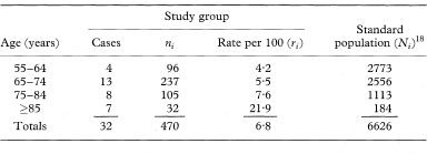
Table 7.8 Paget’s disease of bone in British male migrants to Australia by age group¹⁷

The 95% confidence interval for the population value of the standardised prevalence rate is then given by

that is, from 3·5 to 8·0 per 100.

Comment

Many of the methods described here and others are also given with examples by Rothman and Greenland.¹⁹ Several alternative methods of constructing confidence intervals for standardised rates and ratios have been developed.^20–23 Further discussion of confidence limits for the relative risk can be found in Bailey.²⁴ In particular, a method based on likelihood scores is evaluated by Gart and Nam²⁵ (see also chapter 10). A useful review of approximate confidence intervals for relative risks and odds ratios is given by Sato.²⁶

1 Katz D, Baptista J, Azen SP, Pike MC. Obtaining confidence intervals for the risk ratio in cohort studies. Biometrics 1978;34:469–74.

2 Brenner H, Rothenbacher D, Bode G, Adler G. Parental history of gastric or duodenal ulcer and prevalence of Helicobacter pylori infection in preschool children: population based study. BMJ 1998;316:665.

3 Daly LE. Confidence limits made easy: interval estimation using a substitution method. Am J Epidemiol 1998;147:783–90.

4 Greenland S. Re: “Confidence limits made easy: Interval estimation using a substitution method”. Am J Epidemiol 1999;149:884.

5 Walter SD. The estimation and interpretation of attributable risk in health research. Biometrics 1976;32:829–49.

6 Armitage P, Berry G. Statistical methods in medical research. 3rd edn. Oxford: Blackwell, 1994: 438, 509, 512, 514.

7 Woolf B. On estimating the relationship between blood group and disease. Ann Hum Genet 1955;19:251–3.

8 Breslow NE, Day NE. Statistical methods in cancer research. Volume 1—The analysis of case-control studies. Lyon: International Agency for Research on Cancer, 1980: 124–146, 169–182, 192–246.

9 Shinebaum R, Blackwell CC, Forster PJG, Hurst NP, Weir DM, Nuki G. Nonsecretion of ABO blood group antigens as a host susceptibility factor in the spondyloarthropathies. BMJ 1987;294:208–10.

10 Wald NJ, Nanchahal K, Thompson SG, Cuckle HS. Does breathing other people’s tobacco smoke cause lung cancer? BMJ 1986;293:1217–22.

11 Lentner C, ed. Geigy scientific tables. Volume 2. 8th edn. Basle: Ciba-Geigy, 1982:89–102.

12 Eason J, Markowe HLJ. Controlled investigation of deaths from asthma in hospitals in the North East Thames region. BMJ 1987;294:1255–8.

13 Nunn AJ, Mulder DW, Kamali A, Ruberantwari A, Kengeya-Kayondo J-F, Whitworth J. Mortality associated with HIV-1 infection over five years in a rural Ugandan population: cohort study. BMJ 1997;315:767–71.

14 Breslow NE, Day NE. Statistical methods in cancer research. Volume 2—The design and analysis of cohort studies. Oxford: Oxford University Press, 1988: 69, 93.

15 Roman E, Beral V, Carpenter L, et al. Childhood leukaemia in the West Berkshire and the Basingstoke and North Hampshire District Health Authorities in relation to nuclear establishments in the vicinity. BMJ 1987;294:597–602.

16 Ederer F, Mantel N. Confidence limits on the ratio of two Poisson variables. Am J Epidemiol 1974;100:165–7.

17 Gardner MJ, Guyer PB, Barker DJP. Radiological prevalence of Paget’s disease of bone in British migrants to Australia. BMJ 1978;i:1655–7.

18 Barker DJP, Clough PWL, Guyer PB, Gardner MJ. Paget’s disease of bone in 14 British towns. BMJ 1977;i:1181–3.

19 Rothman KJ, Greenland S. Modern epidemiology. 2nd edn. Philadelphia: Lippincott-Raven, 1998; chapters 14–16.

20 Ulm K. A simple method to calculate the confidence interval of a standardized mortality ratio (SMR). Am J Epidemiol 1990;131:373–5.

21 Sahai H, Khurshid A. Confidence intervals for the mean of a Poisson distribution: a review. Biom J 1993;7:857–67.

22 Fay MP, Feuer EJ. Confidence intervals for directly standardized rates: a method based on the gamma distribution. Statist Med 1997;16:791–801.

23 Kulkarni PM, Tripathi RC, Michalek JE. Maximum (max) and mid-p confidence intervals and p values for the standardized mortality and incidence ratios. Am J Epidemiol 1998;147:83–6.

24 Bailey BJR. Confidence limits to the risk ratio. Biometrics 1987;43:201–5.

25 Gart JJ, Nam J. Approximate interval estimation of the ratio of binomial parameters: A review and corrections for skewness. Biometrics 1988;44:323–38.

26 Sato T. Confidence intervals for effect parameters common in cancer epidemiology. Environ Health Perspect 1990;87:95–101.