
The most common statistical analyses are those that examine one or two groups of individuals with respect to a single variable (see chapters 4 to 7). Also common are those analyses that consider the relation between two variables in one group of subjects. We use regression analysis to predict one variable from another, and correlation analysis to see if the values of two variables are associated. The purposes of these two analyses are distinct, and usually one only should be used.
We outline the calculation of the linear regression equation for predicting one variable from another and show how to calculate confidence intervals for the population value of the slope and intercept of the line, for the line itself, and for predictions made using the regression equation. We explain how to obtain a confidence interval for the population value of the difference between the slopes of regression lines from two groups of subjects and how to calculate a confidence interval for the vertical distance between two parallel regression lines.
We also describe the calculations of confidence intervals for Pearson’s correlation coefficient and Spearman’s rank correlation coefficient.
The calculations have been carried out to full arithmetical precision, as is recommended practice (see chapter 14), but intermediate steps are shown as rounded results. Methods of calculating confidence intervals for different aspects of regression and correlation are demonstrated. The appropriate ones to use depend on the particular problem being studied.
The interpretation of confidence intervals has been discussed in chapters 1 and 3. Confidence intervals convey only the effects of sampling variation on the estimated statistics and cannot control for other errors such as biases in design, conduct, or analysis.
For two variables x and y we wish to calculate the regression equation for predicting y from x. We call y the dependent or outcome variable and x the independent or explanatory variable. The equation for the population regression line is

where A is the intercept on the vertical y axis (the value of y when x = 0) and B is the slope of the line. In standard regression analysis it is assumed that the distribution of the y variable at each value of x is Normal with the same standard deviation, but no assumptions are made about the distribution of the x variable. Sample estimates a (of A) and b (of B) are needed and also the means of the two variables ( and
and  ), the standard deviations of the two variables (sx and sy), and the residual standard deviation of y about the regression line (sres). The formulae for deriving a, b, and sres are given under “Technical details” at the end of this chapter.
All the following confidence intervals associated with a single regression line use the quantity t1 – α/2, the appropriate value from the t distribution with n – 2 degrees of freedom where n is the sample size. Thus, for a 95% confidence interval we need the value that cuts off the top 2·5% of the t distribution, denoted
A fitted regression line should be used to make predictions only within the observed range of the x variable. Extrapolation outside this range is unwarranted and may mislead.1
It is always advisable to plot the data to see whether a linear relationship between x and y is reasonable. In addition a plot of the “residuals” (“observed minus predicted”—see “Technical details” at the end of this chapter) is useful to check the distributional assumptions for the y variable.
Table 8.1 shows data from a clinical trial of enalapril versus placebo in diabetic patients.2 The variables studied are mean arterial blood pressure (mmHg) and total glycosylated haemoglobin concentration (%). The analyses presented here are illustrative and do not relate directly to the clinical trial. Most of the methods for calculating confidence intervals are demonstrated using only the data from the 10 subjects who received enalapril.
Table 8.1 Mean arterial blood pressure and total glycosylated haemoglobin concentration in two groups of 10 diabetics on entry to a clinical trial of enalapril versus placebo2
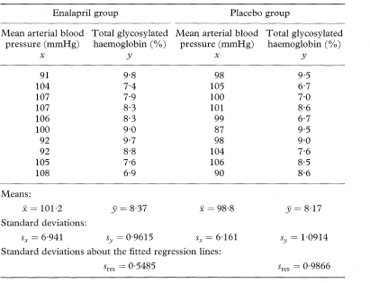
We want to describe the way total glycosylated haemoglobin concentration changes with mean arterial blood pressure. The regression line of total glycosylated haemoglobin (TGH) concentration on mean arterial blood pressure (MAP) for the 10 subjects receiving enalapril is found to be

The estimated slope of the line is negative, indicating lower total glycosylated haemoglobin concentrations for subjects with higher mean arterial blood pressure.
The other quantities needed to obtain the various confidence intervals are shown in Table 8.1. The calculations use 95% confidence intervals. For this we need the value of t0.975 with 8 degrees of freedom, and Table 18.2 shows this to be 2·306.
The slope of the sample regression line estimates the mean change in y for a unit change in x. The standard error of the slope, b, is calculated as

The 100(1 – α)% confidence interval for the population value of the slope, B, is given by


The estimated mean value of y for any chosen value of x, say x0, is obtained from the fitted regression line as

The standard error of yfit is given by

The 100(1 – α)% confidence interval for the population mean value of y at x = x0 is then

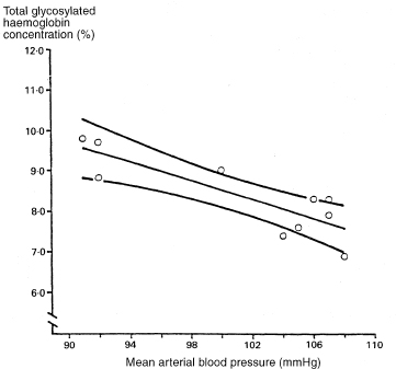
When this calculation is made for all values of x in the observed range of x a 100(1 – α)% confidence interval for the position of the population regression line is obtained. Because of the expression (x0 –  )2 in the formula for SE(yfit) the confidence interval becomes wider with increasing distance of x0 from
  .
.


The intercept of the regression line on the y axis is generally of less interest than the slope of the line and does not usually have any obvious clinical interpretation. It can be seen that the intercept is the fitted value of y when x is zero.
Thus a 100(1 — α)% confidence interval for the population value of the intercept, A, can be obtained using the formula from the preceding section with x0 = 0 and yfit = a. The standard error of a is given by

The confidence interval for a is thus given by

Figure 8.1 Regression line of total glycosylated haemoglobin concentration on mean arterial blood pressure, with 95% confidence interval for the population mean total glycosylated haemoglobin concentration.
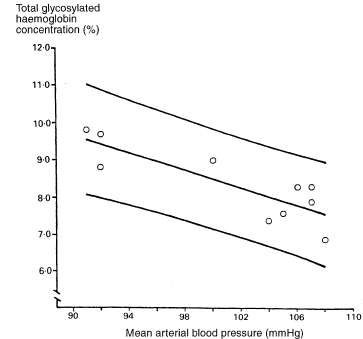
It is useful to calculate the uncertainty in yfit as a predictor of y for an individual. The range of uncertainty is called a prediction (or tolerance) interval. A prediction interval is wider than the asso-ciated confidence interval for the mean value of y because the scatter of data about the regression line is more important. Unlike the confidence interval for the slope, the width of the prediction interval is not greatly influenced by sample size.
For an individual whose value of x is x0 the predicted value of y is yfit, given by

To calculate the prediction interval we first estimate the standard deviation (spred) of individual values of y when x equals x0 as

The 100(1 – α)% prediction interval is then

When this calculation is made for all values of x in the observed range the estimated prediction interval should include the values of y for 100(1 – α)% of subjects in the population.


Regression lines fitted to observations from two independent groups of subjects can be analysed to see if they come from populations with regression lines that are parallel or even coincident.3
If we have fitted regression lines to two different sets of data on the same two variables we can construct a confidence interval for the difference between the population regression slopes using a similar approach to that for a single regression line. The standard error of the difference between the slopes is given by first calculating spool, the pooled residual standard deviation, as
Figure 8.2 Regression line of total glycosylated haemoglobin concentration on mean arterial blood pressure, with 95% prediction interval for an individual total glycosylated haemoglobin concentration.

and then

where the suffixes 1 and 2 indicate values derived from the two separate sets of data. The 100(1 – α)% confidence interval for the population difference between the slopes is now given by

where t1 – α/2 is the appropriate value from the t distribution with n1 + n2 – 4 degrees of freedom.

The difference between the estimated slopes of the two regression lines is –0·1168 – (–0·09268) = –0·02412%. The standard error of this difference is found by first calculating spool as


If the chosen confidence interval—for example., 95%—for the difference between population values of the slopes includes zero it is reasonable to fit two parallel regression lines with the same slope and calculate a confidence interval for their common slope. In practice we would usually perform this analysis by multiple regression using a statistical software package (see below). The calculation can be done, however, using the results obtained by fitting separate regression lines to the two groups and the standard deviations of the x and y values in the two groups: sx1, sx2, sy1, and sy2. First we define the quantity w as

The common slope of the parallel lines (bpar) is estimated as

The residual standard deviation of y around the parallel lines (spar) is given by

and the standard error of the slope by

The 100(1 – α)% confidence interval for the population value of the common slope is then

where t1 – α/2 is the appropriate value from the t distribution with n1 + n2 – 3 degrees of freedom.


The intercepts of the two parallel lines with the y axis are given by

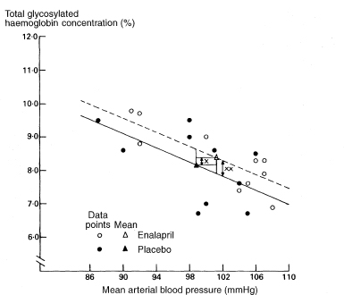
We are usually more interested in the difference between the intercepts., which is the vertical distance between the parallel lines. This is the same as the difference between the fitted y values for the two groups at the same value of x, and is equivalent to adjusting the observed mean values of y for the mean values of x, a method known as analysis of covariance.3 The adjusted mean difference (ydiff) is calculated as

and the standard error of ydiff is

The 100(1 – α)% confidence interval for the population value of ydiff is then

where t1 – α/2 is the appropriate value from the t distribution with n1 + n2 – 3 degrees of freedom.


Figure 8.3 llustration of the calculation of the adjusted difference between mean total glycosylated haemoglobin concentrations in two groups.
Differences between means:
×, observed difference =  1 –
1 –  2 = 0·20%;
× ×, adjusted difference = ydiff = 0·45%.
The methods described for two groups can be extended to the case of more than two groups of individuals,3 although such problems are rather rare. The calculations are best done using software for multiple regression, as discussed below.
We have shown linear regression with a continuous explanatory variable but this is not a requirement. Regression with a single binary explanatory variable is equivalent to performing a two-sample t test. When several explanatory variables are considered at once using multiple regression, as described below, it is common for some to be binary.
In many studies the outcome variable of interest is the presence or absence of some condition, such as responding to treatment or having a myocardial infarction. When we have a binary outcome variable and give the categories numerical values of 0 and 1, usually representing “No” and “Yes” respectively, then the mean of these values in a sample of individuals is the same as the proportion of individuals with the characteristic. We might expect, therefore, that the appropriate regression model would predict the proportion of subjects with the feature of interest (or, equivalently, the probability of an individual having that characteristic) for different values of the explanatory variable.
The basic principle of logistic regression is much the same as for ordinary multiple regression. The main difference is that the model predicts a transformation of the outcome of interest. If p is the proportion of individuals with the characteristic, the transformation we use is the logit transformation, logit(p) = log[p/(1 – p)]. The regression coefficient for an explanatory variable compares the estimated outcome associated with two values of that variable, and is the log of the odds ratio (see chapter 7). We can thus use the model to estimate the odds ratio as eb, where b is the estimated regression coefficient (log odds ratio). A confidence interval for the odds ratio is obtained by applying the same transformation to the confidence interval for the regression coefficient. An example is given below, in the section on multiple regression.
The regression method introduced by Cox in 1972 is used widely when the outcome is the time to an event.4 It is also known as proportional hazards regression analysis. The underlying methodology is complex, but the resulting regression model has a similar interpretation to a logistic regression model. Again the explanatory variable could be continuous or binary (for example, treatment in a randomised trial).
In this model the regression coefficient is the logarithm of the relative hazard (or “hazard ratio”) at a given time. The hazard represents the risk of the event in a very short time interval after a given time, given survival that far. The hazard ratio is interpreted as the relative risk of the event for two groups defined by different values of the explanatory variable. The model makes the strong assumption that this ratio is the same at all times after the start of follow up (for example, after randomisation in a controlled trial).
We can use the model to estimate the hazard ratio as eb, where b is the estimated regression coefficient (log hazard ratio). As for logistic regression, a confidence interval is obtained by applying the same transformation to the confidence interval for the regression coefficient. An example is given below, in the section on multiple regression. A more detailed explanation of the method is given in chapter 9.
In much medical research there are several potential explanatory variables. The principles of regression—linear, logistic, or Cox— can be extended fairly simply by using multiple regression.4 Further, the analysis may include binary as well as continuous explanatory variables. Standard statistical software can perform such calculations in a straightforward way. There are many issues relating to such analysis that are beyond the scope of this book—for discussion see, for example, Altman.4
Although the nature of the prediction varies according to the model, in each case the multiple regression analysis produces a regression equation (or “model”) which is effectively a weighted combination of the explanatory variables. The regression coefficients are the weights given to each variable.
For each variable in the regression model there is a standard error, so that it is easy to calculate a confidence interval for any particular variable in the model, using the standard approach of chapter 3.
The multiple linear regression model is

where Y is the outcome variable, X1 to Xk are k explanatory variables, b0 is a constant (intercept), and b1 to bk are the regression coefficients. The nature of the predicted outcome, Y, varies according to the type of model, as discussed above, but the regression model has the same form in each case. The main difference in multiple regression is that the relation between the outcome and a particular explanatory variable is “adjusted” for the effects of other variables.
The explanatory variables can be either continuous or binary. Table 8.2 shows the interpretation of regression coefficients for different types of outcome variable and for either continuous or binary explanatory variables. For binary variables it is assumed that these have numerical codes that differ by one; most often these are 0 and 1.
Table 8.2 Interpretation of regression coefficients for different types of outcome variable and for either continuous or binary explanatory variables

For multiple logistic regression models the regression coefficients and their confidence intervals need to be exponentiated (antilogged) to give the estimated odds ratio and its confidence interval. The same process is needed in Cox regression to get the estimated hazard ratio with its confidence interval.
Table 8.3 shows a multiple logistic regression model from a study of 183 men with unstable angina.5 The regression coefficients and confidence intervals have been converted to the odds ratio scale.
Some points to note about this analysis are:
Table 8.3 Logistic regression model for predicting cardiac death or non-fatal myocardial infarction.5

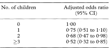
Table 8.4 Association between number of children and risk of testicular cancer in Danish men (514 cases and 720 controls)6
The correlation coefficient usually calculated is the product moment correlation coefficient or Pearson’s r. This measures the degree of linear ‘co-relation’ between two variables x and y. The formula for calculating r for a sample of observations is given at the end of the chapter.
A confidence interval for the population value of r can be constructed by using a transformation of r to a quantity Z, which has an approximately Normal distribution. This calculation relies on the assumption that x and y have a joint bivariate Normal distribution (in practice, that the distributions of both variables are reasonably Normal).
The transformed value, Z, is given by

which for all values of r has SE = 1 /  where n is the sample size. For a 100(1 – α)% confidence interval we then calculate the two quantities

where z1 – α/2 is the appropriate value from the standard Normal distribution for the 100(1 – α/2)% percentile (Table 18.1).
The values F and G need to be transformed back to the original scale to give a 100(1 – α)% confidence interval for the population correlation coefficient as


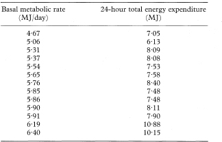
Table 8.5 Basal metabolic rate and isotopically measured 24-hour energy expenditure in 13 non-obese women7


If either the distributional assumptions are not met or the relation between x and y is not linear we can use a rank method to assess a more general relation between the values of x and y. To calculate Spearman’s rank correlation coefficient (rs) the values of x and y for the n individuals have to be ranked separately in order of increasing size from 1 to n. Spearman’s rank correlation coefficient is then obtained either by using the standard formula for Pearson’s product moment correlation coefficient on the ranks of the two variables, or (as shown below under “Technical details”) using the difference in their two ranks for each individual. The distribution of rs similar to that of Pearson’s r, so that confidence intervals can be constructed as shown in the previous section.
We strongly recommend that statistical software is used to perform regression or correlation analyses. Some formulae are given here to help explain the underlying principles.
The slope of the regression line is given by

where ∑ represents summation over the sample of size n. The intercept is given by

The difference between the observed and predicted values of y for an individual with observed values x0 and y0 is y0 – yfit, where yfit = a + bx0. The standard deviation of these differences (called “residuals”) is thus a measure of how well the line fits the data.
The residual standard deviation of y about the regression line is
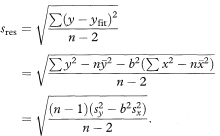
Most statistical computer programs give all the necessary quantities to derive confidence intervals, but you may find that the output refers to sres as the ‘standard error of the estimate’.
The correlation coefficient (Pearson’s r) is estimated by

Spearman’s rank correlation coefficient is given by

where di is the difference in the ranks of the two variables for the ith-individual. Alternatively, rs can be obtained by applying the formula for Pearson’s r to the ranks of the variables. The calculation of rs should be modified when there are tied ranks in the data, but the effect is minimal unless there are many tied ranks.
1 Altman DG, Bland JM. Generalisation and extrapolation. BMJ 1998;317:409–10.
2 Marre M, Leblanc H, Suarez L, Guyenne T-T, Ménard J, Passa P. Converting enzyme inhibition and kidney function in normotensive diabetic patients with persistent micro-albuminuria. BMJ 1987;294:1448–52.
3 Armitage P, Berry G. Statistical methods in medical research. 3rd edn. Oxford: Blackwell Science, 1994: 336–7.
4 Altman DG. Practical statistics for medical research. London: Chapman & Hall, 1991: 336–58.
5 Stubbs P, Collinson P, Moseley D, Greenwood T, Noble M. Prospective study of the role of cardiac troponin T in patients admitted with unstable angina. BMJ 1996;313:262–4.
6 Møller H, Skakkebæk NE. Risk of testicular cancer in subfertile men: case-control study. BMJ 1999;318:559–62.
7 Prentice AM, Black AE, Coward WA, et al. High levels of energy expenditure in obese women. BMJ 1986;292:983–7.