Studies evaluating diagnostic test performance yield a variety of numerical results. While these ought to be accompanied by confidence intervals, this is less commonly done than in other types of medical research.1
Diagnosis may be based either on the presence or absence of some feature or symptom, on a classification into three or more groups (perhaps using a pathological grading system), or on a measurement. Values of a measurement may also be grouped into two or more categories, or may be kept as measurements. Each case will be considered in turn. See Altman2 for more detailed discussion of most of these methods.
A confidence interval indicates uncertainty in the estimated value. As noted in earlier chapters, it does not take account of any additional uncertainty that might relate to other aspects such as bias in the study design, a common problem with studies evaluating diagnostic studies.3
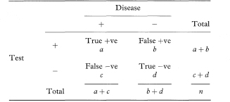
The simplest diagnostic test is one where the results of an investigation, such as an X-ray or biopsy, are used to classify patients into two groups according to the presence or absence of a symptom or sign. The question is then to quantify the ability of this binary test to discriminate between patients who do or do not have the disease or condition of interest. (The general term “disease” is used here, although the target disorder is not always a disease.) Table 10.1 shows a 2 × 2 table representing this situation, in which a, b, c, and d are the numbers of individuals in each cell of the table.
Table 10.1 Relation between a binary diagnostic test and presence or absence of disease

The two most common indices of the performance of a test are the sensitivity and specificity. The sensitivity is the proportion of true positives that are correctly identified by the test, given by a/(a + c) in Table 10.1. The specificity is the proportion of true negatives that are correctly identified by the test, or d/(b + d).
The sensitivity and specificity are proportions, and so confidence intervals can be calculated for them using the traditional method or Wilson’s method, as discussed in chapter 6. Note that the traditional method may not perform well when proportions are close to 1 (100%) as is often the case in this context, and may even give confidence intervals which exceed 100%.4 Wilson’s method is thus generally preferable.
Table 10.2 Results of ice-water test among patients with either detrusor hyperreflexia (DH) or bladder instability (BI)5
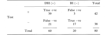
In clinical practice the test result is all that is known, so we want to know how good the test is at predicting abnormality. In other words, what proportion of patients with abnormal test results are truly abnormal? The sensitivity and specificity do not give us this information. Instead we must approach the data from the direction of the test results. These two proportions are defined as follows:
In the notation of Table 10.1, PV + = a/(a + b) and PV – = d/(c + d).
We should not stop the analysis here. The predictive values of a test depend upon the prevalence of the abnormality in the patients being tested, which may not be known. The values just calculated assume that the prevalence of detrusor hyperreflexia among the population of patients likely to be tested is the same as in the sample, namely 60/80 or 75%. In a different clinical setting the prevalence of abnormality may differ considerably.
Predictive values observed in one study do not apply universally. The rarer the true abnormality is, the more sure we can be that a negative test indicates no abnormality, and the less sure that a positive result really indicates an abnormal patient.
More general formulae for calculating predictive values for any prevalence (prev) are

and

where sens and spec are the sensitivity and specificity as previously defined. The prevalence can be interpreted as the probability before the test is carried out that the subject has the disease, also known as the prior probability of disease. PV+ and PV– are the revised estimates of the probability of disease for those subjects who are positive and negative to the test, and are known as posterior probabilities. The comparison of the prior and posterior probabilities is one way of assessing the usefulness of the test. The predictive values can change considerably with a different prevalence.
We can obtain approximate confidence intervals for prevalence- adjusted predictive values by expressing them as proportions of the number of positive or negative test results in the study.

For any test result we can compare the probability of getting that result, if the patient truly had the condition of interest, with the corresponding probability if they were healthy. The ratio of these probabilities is called the likelihood ratio (LR). The likelihood ratio for a positive test result is calculated as

and the likelihood ratio for a negative test result is calculated as

The contrast between these values indicates the value of the test for increasing certainty about a diagnosis.2
The likelihood ratio is increasingly being quoted in papers describing diagnostic test results, but is rarely accompanied by a confidence interval. The likelihood ratio for a positive test can be also expressed as the ratio of the true-positive and false-positive rates., that is

Similarly, the likelihood ratio for a negative test can be expressed as the ratio of the true-negative and false-negative rates, that is

The likelihood ratio is identical in construction to a relative risk (or risk ratio)—that is, it is the ratio of two independent proportions. It follows immediately that a method for deriving a confidence interval for a relative risk can be applied also to the likelihood ratio. There are several possible methods, not all of which are equally good. Two are considered here.
Confidence intervals for the population value of the likelihood ratio can be constructed through a logarithmic transformation,2 as described in chapter 7. The method is illustrated using LR+. The standard error of loge LR+ is

from which a 100(1 – α)% confidence interval for logeLR+ is found in the standard way. We obtain a confidence interval for LR+ by antilogging (exponentiating) these values. (The derivation of this method, sometimes called the log method, is given in the appendix of Simel et al.6)
Note that either a or b can be zero, in which case SE(loge LR+) becomes infinite. To avoid this problem, it may be preferable in such cases to add 0·5 to the counts in all four cells of the observed table before calculating both LR+ and SE(loge LR+).
The “score test” method reportedly performs somewhat better that the usual log method,7,8 although it is too complex for the formula to be given here.
Multicategory classifications represent an intermediate step between dichotomous tests and tests based on measurements. With few categories, say three or four, we can evaluate the preceding statistics using in turn each division between categories to create a binary test. Sometimes this procedure is adopted for tests which are measurements. For example, Sackett et al.10 discuss the use of serum ferritin level in five bands to diagnose, or rule out, iron-deficiency anaemia.
Many diagnostic tests are quantitative, notably in clinical chemistry. The methods of the preceding sections can be applied only if we can select a cutpoint to distinguish “normal” from “abnormal”, which is not a trivial problem. It is often done by taking the observed median value, or perhaps the upper limit of a predetermined reference interval.
This approach is wasteful of information, however, and involves a degree of arbitrariness. Classification into several groups is better than just two, but there are ways of proceeding that do not require any grouping of the data; they are described in this section.
First we can investigate to what extent the test results differ among people who do or do not have the diagnosis of interest. The receiver operating characteristic (ROC) plot is one way to do this. ROC plots were developed in the 1950s for evaluating radar signal detection. A paper by Hanley and McNeil11 was very influential in introducing the method to medicine.
The ROC plot is obtained by calculating the sensitivity and specificity for every distinct observed data value and plotting sensitivity against 1 – specificity, as in Figure 10.1. A test that discriminates perfectly between the two groups would yield a “curve” that coincided with the left and top sides of the plot. A test that is completely useless would give a straight line from the bottom left corner to the top right corner. In practice the ROC curve will lie somewhere between these extremes according to the degree of overlap of the values in the groups.
Figure 10.1 ROC curve for data in Table 10.3.
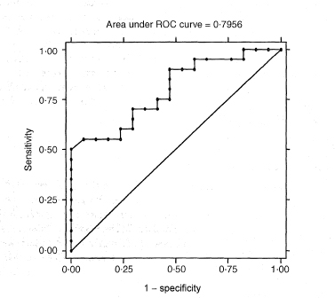
A global assessment of the performance of the test, sometimes called diagnostic accuracy,12 is given by the area under the ROC curve (often abbreviated AUC). This area is equal to the probability that a random person with the disease has a higher value of the measurement than a random person without the disease. The area is 1 for a perfect test and 0·5 for an uninformative test. The non-parametric calculation of the area under the curve is closely related to the Mann-Whitney U statistic.
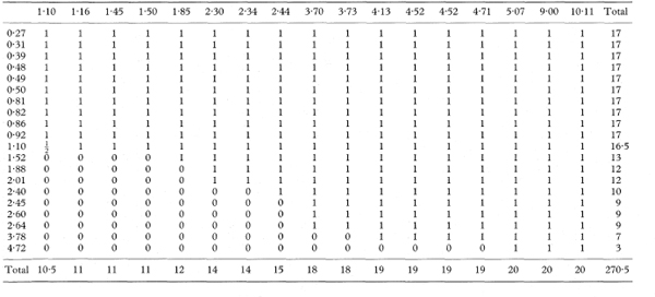
The area under the curve and its standard error can be obtained by examining every comparison of a member of each group. We consider the n individuals in the first group with values Xi and the m individuals in the second group with observations Yj, so that there are nm pairs of values Xi and Yj. For each pair we obtain a “placement score” ψij, which indicates which value is larger. We have ψij = 1 if Yj > Xi; ψij = 0·5 if Yj = Xi; and ψij = 0 if Yj < Xi. In effect we assess where each observation is placed compared with all of the values in the other group.14,15.
The area under the curve is simply the mean of all of the values ψij. In mathematical notation, we have

The area under the curve can also be written as

where

The values Ri indicate for each member of the first group the proportion of the observations in the second group which exceed it, and similarly for Cj. (They are also the row and column totals of ψij when the data are arranged in a two-way table, as in the worked example below.)
To get the standard error of AUC we first calculate the quantities

and

The standard error of AUC is then given by

An equivalent method, based on the values of Ri and Cj, and avoiding the need to calculate  and
and  is
is

where var indicates the variance. The standard error of AUC, the area under the ROC curve, can be used to construct a confidence interval in the familiar way using the general formula given in chapter 3. A 100(1 – α)% confidence interval for AUC is

where z1 – α/2 is the appropriate value from the standard Normal distribution for the 100(1 – α/2) percentile (see Table 18.1). For a 95% confidence interval, z1 – α/2 = 1·96.
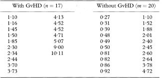
Table 10.3 Values of an index of mixed epidermal cell lym-phocyte reactions in bone-marrow transplant recipients who did or did not develop graft-versus-host disease (GvHD)13

The method just described relies on the assumption that the area under the curve has a Normal sampling distribution. Obuchowski and Lieber16 note that for methods of high accuracy (AUC > 0·95) use of the preceding method for the area under a single ROC curve may require a sample size of 200. For smaller samples a bootstrap approach is recommended (see chapter 13).
Having determined that a test does provide good discrimination the choice can be made of the best cutpoint for clinical use. The simple approach of minimising “errors” (equivalent to maximising the sum of the sensitivity and specificity) is common, but it is not necessarily best. Consideration needs to be given to the costs (not just financial) of false-negative and false-positive diagnoses, and the prevalence of the disease in the subjects being tested.12 For example, when screening the general population for cancer the cutpoint would be chosen to ensure that most cases were detected (high sensitivity) at the cost of many false positives (low specificity), who could be eliminated by a further test.
Table 10.4 Placement scores (ψij) for the data in Table 10.3
The ROC plot is more useful when comparing two or more measures. A test with a curve that lies wholly above the curve of another will be clearly better. Methods for comparing the areas under two ROC curves for both paired and unpaired data are reviewed by Zweig and Campbell.12
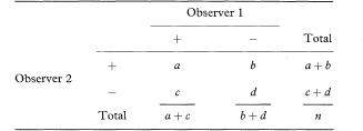
An important aspect of classifying patients into two or more categories is the consistency with which it can be done. Of particular interest here is the ability of different observers to agree on the classification. A similar situation arises when we wish to compare two alternative diagnostic tests to see how well they agree with each other. In each case, we can construct a two-way table such as Table 10.5 and compare the observed agreement with that which we would expect by chance alone, using the statistic known as kappa (K).
Kappa is a measure of agreement beyond the level of agreement expected by chance alone. The observed agreement is the proportion of samples for which both observers agree, given by po = (a + d)/n. To get the expected agreement we use the row and column totals to estimate the expected numbers agreeing for each category. For positive agreement (+, +) the expected proportion is the product of (a + b)/n and (a + c)/n, giving (a + b)(a + c)/n2. Likewise, for negative agreement the expected proportion is (c + d)(b + d)/n2. The expected proportion of agreements for the whole table (pe) is the sum of these two terms. From these elements we obtain kappa as

Table 10.5 Comparison of binary assessments by two observers
and its standard error is

from which a 100(1 – α)% confidence interval for K is found in the standard way as

where z1 – α/2 is defined as above.
Kappa has its maximum value of 1 when there is perfect agreement. A kappa value of 0 indicates agreement no better than chance, while negative values (rarely encountered) indicate agreement worse than chance.


Table 10.6 Comparison of paediatrician’s and parent’s assessments of whether children could walk downstairs17

The calculation of kappa can be extended quite easily to assessments with more than two categories.2 If there are g categories and fi is the number of agreements for the ith category, then the overall observed agreement is

If ri and ci are the totals of the ith row and ith column, then the overall expected agreement is

Kappa and its standard error are then calculated as before.
Kappa can also be extended to multiple observers, and it is possible to weight the disagreements according to the number of categories separating the two assessments.
1 Harper R, Reeves B. Reporting of precision of estimates for diagnostic accuracy: a review. BMJ 1999;318:1322–3.
2 Altman DG. Practical statistics for medical research. London: Chapman & Hall, 1991:403–19.
3 Reid MC, Lachs MS, Feinstein AR. Use of methodological standards in diagnostic test research. JAMA 1995;274:645–51.
4 Deeks JJ, Altman DG. Sensitivity and specificity and their confidence intervals cannot exceed 100. BMJ 1999;318:193–4.
5 Petersen T, Chandiramani V, Fowler CJ. The ice-water test in detrusor hyperreflexia and bladder instability. Br J Urol 1997;79:163–7.
6 Simel DL, Samsa GP, Matchar DB. Likelihood ratios with confidence: sample size estimation for diagnostic test studies. J Clin Epidemiol 1991;44:763–70.
7 Gart JJ, Nam J. Approximate interval estimation of the ratio of binomial proportions: a review and corrections for skewness. Biometrics 1988;44:323–38.
8 Nam J. Confidence limits for the ratio of two binomial proportions based on likelihood scores: non-iterative method. Biom J 1995;37:375–9.
9 Koopman PAR. Confidence limits of the ratio of two binomial proportions. Biometrics 1984;80:513–17.
10 Sackett DL, Richardson WS, Rosenberg W, Haynes RB. Evidence-based medicine. How to practise and teach EBM. London: Churchill-Livingstone, 1997:124.
11 Hanley JA, McNeil BJ. The meaning and use of the area under a receiver operating characteristic (ROC) curve. Radiology 1982;143:29–36.
12 Zweig MH, Campbell G. Receiver-operating characteristic (ROC) plots: a fundamental tool in clinical medicine. Clin Chem 1993;39:561–77.
13 Bagot M, Mary J-Y, Heslan M et al. The mixed epidermal cell lymphocyte reaction is the most predictive factor of acute graft-versus-host disease in bone marrow graft recipients. Br J Haematol 1988;70:403–9.
14 DeLong ER, DeLong DM, Clarke-Pearson DL. Comparing the areas under two or more correlated receiver operating characteristic curves: a nonparametric approach. Biometrics 1988;44:837–45.
15 Hanley JA, Haijan-Tilaki KO. Sampling variability of nonparametric estimates of the areas under receiver operating characteristic curves: an update. Acad Radiol 1997;4:49–58.
16 Obuchowski NA, Lieber ML. Confidence intervals for the receiver operating characteristic area in studies with small samples. Acad Radiol 1998;5:561–71.
17 Fooks J, Mutch L, Yudkin P, Johnson A, Elbourne D. Comparing two methods of follow up in a multicentre randomised trial. Arch Dis Child 1997;76:369–76.