11

Clinical trials and meta-analyses

DOUGLAS G ALTMAN

Confidence intervals are of special importance in the interpretation of the results of randomised clinical trials. The decision about whether or not to adopt a particular treatment is aided by knowledge of the uncertainty of the treatment effect. Most of the necessary statistical methods have been presented in earlier chapters. Here their relevance to controlled trials will be pointed out and confidence intervals for a few further measures introduced. The use of confidence intervals in meta-analyses of the data from several randomised trials is also considered.

I shall assume that two treatments are being compared. These are referred to as treatment and control, where the control group may receive an active treatment, no treatment, or placebo. There are some comments on the case of more than two groups in chapter 13.

The confidence interval indicates uncertainty in the estimated treatment effect arising from sampling variation. Note again that it does not take account of any additional uncertainty that might relate to other aspects such as the non-representativeness of the patients in a randomised trial or the studies in a meta-analysis.

Randomised controlled trials

I consider first trials using a parallel group design and then trials using the crossover design.

Parallel group trials

Continuous outcome

When the outcome is a continuous measure, such as blood pressure or lung function, the usual analysis is a comparison of the observed mean (or perhaps mean change from baseline) in the two treatment groups, using the method based on the t distribution (chapter 4).

Worked example

A randomised controlled trial compared intermittent cyclical etidronate with placebo in patients undergoing long-term oral corticosteroid therapy. The groups were compared with respect to percentage change in lumbar spine bone mineral density after two years.¹ The mean percentage increase in bone mineral density was 5·12% (SD 4·67%) in 21 etidronate-treated patients and 0·98% (SD 5·88%) in 16 placebo-treated patients. (Note that some “increases” were negative.) Using the method described in chapter 4, the mean difference between the two groups was 4·14% with standard error 1·733%. The value of t_0.975 with 21 + 16 – 2 = 35 degrees of freedom is 2·030. A 95% confidence interval for the difference between the groups is thus

that is, 0·62% to 7·66%.

If the data within each treatment group are not close to having a Normal distribution, we may need to make a log transformation of the data before analysis (described in chapter 4) or use a nonparametric method (described in chapter 5).

Binary outcome

Many trials have outcomes that are binary, often indicating whether or not the patient experienced a particular event (such as a myocardial infarction or resolution of the illness). When the outcome is binary, there are three statistics commonly used to summarise the treatment effect—the risk difference, the relative risk, and the odds ratio. Methods for constructing confidence intervals for all of these measures were presented in chapters 6 and 7; here I recast them in the context of clinical trials. None of them is uniformly the most appropriate. However, the odds ratio is not an obvious effect measure for a randomised trial, and it may mislead when events are common (say >30% of patients).²

The data from a controlled trial can be presented as in Table 11.1. The observed proportions experiencing the event are p_T = a/n_T and p_C = b/n_C The risk difference (also called the absolute risk reduction) is given by p_T – p_C or p_C – p_T, whichever is more appropriate. The appropriate confidence interval is that for the difference between two proportions, as given in chapter 6.

Table 11.1 Patient outcome by treatment group

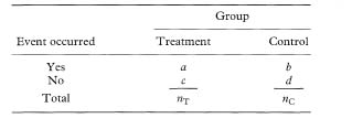
The relative risk (also called the risk ratio) (RR) is defined as the ratio of the event rates, either P_T/P_C or P/P_T. The odds ratio (OR) is defined as p_T(1 – P_C)/P_C(1 – P_T); it is more easily obtained as ad/bc. Confidence intervals for both the relative risk and odds ratio were given in chapter 7 in the sections on incidence studies and unmatched case-control studies respectively.

Worked example

Rai et al.³ carried out a randomised controlled trial of aspirin plus heparin versus aspirin in pregnant women with recurrent miscarriage. The proportions of women having a successful live birth was 32/45 (71%) in the aspirin plus heparin group and 19/45 (42%) in the aspirin only group. The relative risk of a live birth was thus R = (32/45)/(19/45) = 1·68 and log_e R = 0·226. Using the method in chapter 7, the standard error of the log relative risk is given by

The 95% confidence interval for log_e R is thus 0·132 to 0·911 and the 95% confidence interval for the relative risk is obtained as e⁰·¹³² to e⁰·⁹¹¹, or 1·14 to 2·49.

The term “relative risk” is more often used when the outcome is an adverse one. In this trial we could calculate the relative risk of failing to have a live birth. The relative risk is now (13/45)/(26/45) = 0·5, indicating a halving of the risk of an adverse outcome. A 95% confidence interval for log_e R is –1·215 to –0·171, and the 95% confidence interval for the relative risk is 0·30 to 0·84. These values cannot be obtained simply from those for the relative risk of a live birth.

Some authors present results using the odds ratio. This has the advantage that it gives a unique answer whether one takes a good or bad outcome. But, as noted above, it may be misleading when events are common as here. In their paper, Rai et al³ gave the odds ratio for a live birth as 3·37 (95% confidence interval 1·40 to 8·10). Because live births were common the odds ratio is much larger than the corresponding relative risk of 1·68. Interpreted (wrongly) as a relative risk it would imply an effect twice the size of the true one.

When the treatment of interest reduces the risk of an adverse event, so that the relative risk or odds ratio is less than 1, it may be useful to present the relative risk reduction or relative odds reduction, defined as 1 – RR or 1 – OR, with a confidence interval. These values are sometimes multiplied by 100 to give percentages. In each case, the confidence interval is obtained by making the same manoeuvre. In the above study, the relative risk of not having a live birth was 0·50 with 95% confidence interval from 0·30 to 0·84. This translates into a relative risk reduction of 50% with 95% confidence interval from 16% to 70%.

A further way of quantifying the treatment effect from trials with a binary outcome is the number needed to treat. I discuss this concept later in this chapter.

Outcome is time to an event

In many studies with a binary outcome the focus of interest is not just whether an event occurred but also when it occurred. The methods used to analyse such data go under the general name of survival analysis, regardless of whether the outcome is death or something else. A better general name is thus analysis of time to event data (see chapter 9).

The outcome in such studies is often summarised as the median survival time in each group. The treatment effect is not usually summarised as the difference between these medians, however. It is not simple to provide a confidence interval, and medians often cannot be estimated when the event rate is low. Rather, it is more common to present the hazard ratio, estimated in one of the ways described in chapter 9.

Adjusting for other variables

In some trials there is ancillary information about patients which may influence the observed treatment effect. In particular, many trials with continuous outcomes collect baseline measurements of the variable that the treatment is intended to influence. The best approach for incorporating baseline values into the analysis is to use the baseline value as a predictor (covariate) in a multiple regression analysis,⁴ as described in chapter 8. In other words, we perform a multiple regression of the final value on the treatment (as a binary indicator) and the baseline value. This analysis is sometimes called analysis of covariance; it was used in the etidronate study described earlier.¹ The regression coefficient and confidence interval from the multiple regression analysis give the adjusted treatment effect.

Other (possibly) prognostic variables are handled in the same way, being entered as explanatory variables in a multiple regression analysis. An example was given in Figure 8.3. This more general situation applies to all types of outcome and hence also to logistic and Cox regression models for binary and survival time outcomes respectively (see chapter 8). The choice of which variables to adjust for should ideally be specified in the study protocol, not by which variables seem to differ at baseline between the treatment groups.⁵

The number needed to treat

The valuable concept of the number needed to treat (NNT) was introduced by Laupacis et al.⁶ as an additional way of assessing the treatment benefit from trials with a binary outcome. It has become popular as a useful way of reporting the results of clinical trials,⁷ especially in journals of secondary publication (such as ACP Journal Club and Evidence-Based Medicine).

From the result of a randomised trial comparing a new treatment with a standard treatment, the NNT is the number of patients who need to be treated with the new treatment rather than the standard (control) treatment in order for one additional patient to benefit. It can be obtained for any trial that has reported a binary outcome.

The NNT is calculated as the reciprocal of the risk difference (absolute risk reduction, or ARR), given by 1/(P_C – P_T) (or 1/(P_T – P_C) if the outcome is beneficial to the patient). A large treatment effect thus leads to a small NNT. A treatment which will lead to one saved life per 10 patients treated is clearly better than a competing treatment that saves one life for every 50 treated. When there is no treatment effect the risk difference is zero and the NNT is infinite.

A confidence interval for the NNT is obtained simply by taking reciprocals of the values defining the confidence interval for the absolute risk reduction (see chapter 6). To take an example, if the risk difference in a trial is 10% with a 95% confidence interval from 5% to 15%, the NNT is 1/0·1 = 10 and the 95% confidence interval for the NNT is 6·7 to 20 (i.e. 1/0·15 to 1/0·05).

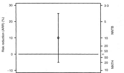
The case of a treatment effect that is not significant is more difficult. The same finding of ARR = 10% with a wider 95% confidence interval for the ARR of –5% to 25% gives the 95% confidence interval for the NNT of 10 as –20 to 4. There are two difficulties with this interval: first, the NNT can only be positive, and second the confidence interval does not seem to include the best estimate of 10. To avoid such perplexing results, the NNT is often given without a confidence interval when the treatments are not statistically significantly different. This is unsatisfactory behaviour, and goes against advice that the confidence interval is especially useful when the result of a trial is not statistically significant (chapter 14). In fact, a sensible confidence interval can be quoted for any trial.

In the example, the 95% confidence interval for the NNT was –20 to 4. The value of –20 indicates that if 20 patients are treated with the new treatment one fewer would have a good outcome than if they all received the standard treatment. In this case the inverse of the ARR is the number of patients treated for one to be harmed. This has been termed the number needed to harm (NNH).^{8, 9} However, it is more appropriate to indicate the number needed to treat for benefit (NNTB) or harm (NNTH). Using these descriptors, the value of –20 corresponds to a NNTH of 20. The confidence interval can thus be rewritten as NNTH 20 to NNTB 4. As already noted, this interval does not seem to include the overall estimate of NNTB 10.

The 95% confidence interval for the ARR includes all values of the ARR from –5% to +25%, including zero. The NNT is infinity (∞) when the ARR is zero, so the confidence interval calculated as NNTH 20 to NNTB 4 must include infinity. The confidence interval is thus most peculiar, comprising values of NNTB from 4 to infinity and values of NNTH from 20 to infinity. Figure 11.1 shows the ARR and 95% confidence interval for the example. The values NNTB = 1 and NNTH = 1 thus correspond to impossible absolute risk reductions of +100% and –100% respectively, and are not actually shown. Conversely, the midpoint on the NNT scale is the case where the treatment makes no difference (ARR = 0 and NNT = ∞). We need to remember the absolute risk reduction scale when trying to interpret the NNT and its confidence interval.

It is desirable to give a confidence interval for the NNT even when the confidence interval for the absolute risk reduction includes zero. I suggest that it is done as, for example, NNTB 10 (95% confidence interval NNTH 20 to ∞ to NNTB 4).

Figure 11.1 Relation between absolute risk reduction and number needed to treat and their confidence intervals for the example discussed in the text.

Example

Tramèr et al.¹⁰ quoted an NNT of –12·5 for a trial comparing the antiemetic efficacy of intravenous ondansetron and intravenous droperidol. The negative NNT implies here that ondansetron was less effective than droperidol. The quoted 95% confidence interval was –3·7 to oo, which is incomplete. The ARR was –0·08 with 95% confidence interval –0·27 to 0.11. We can convert this finding to the NNT scale as NNTH – 12.5 (95% confidence interval NNTH 3·7 to ∞ to NNTB 9·1). With this presentation we can see that an NNTB smaller (better) than 9·1 is unlikely.

The NNT can also be obtained for survival analysis. For these studies the NNT is not a single number, but varies according to time since the start of treatment.¹¹

Benefit per 1000 patients

One of the arguments for using the NNT rather than the absolute risk difference is that the latter is harder to assimilate. For example, it is felt that an NNT of, say, 17 is easier to judge (and remember) than the equivalent absolute risk reduction of 5.9%. One way of representing differences between proportions that has some of the appeal of the NNT is to convert to the number of patients out of 1000 who would benefit from the new treatment. Even though this change is trivial, being achieved simply by multiplying by 10, it does simplify the results. For this measure, of course, a larger number is better.

For example, among patients randomised to streptokinase or placebo within 6 hours of their myocardial infarction, the survival rates by 35 days were 91·8% and 87·5% respectively.¹² The risk difference was thus 4·3% (95% confidence interval 2·1% to 6·5%). Baigent et al.¹² reported this result as 43 patients out of 1000 benefiting from streptokinase (95% confidence interval 21 to 65).

Crossover trials

In crossover trials patients are randomised to groups which receive each treatment in a different sequence. In the most common case, two treatments are given in one of two orders (randomly chosen for each participant), often with a “washout” period in between. The strength of the crossover design is that the two treatments are compared on the same patients rather than on two separate groups. With such trials there is no issue of comparability of groups, but there are other methodological and practical difficulties;¹³ I will not dwell upon them here. Exactly the same analysis issues (and similar methodological problems) arise in within-person randomised trials.

The main difference from parallel group trials is the need to use an analysis that takes account of the paired responses for each patient in the trial. As for parallel group trials, it is essential that the confidence interval relates to the difference between treatments, not separately for the average effects with each of the treatments.

Continuous outcome

For continuous outcomes a confidence interval for the treatment effect is obtained using the method for paired continuous data presented in chapter 4.

Binary outcome

Paired binary data can be presented as in Table 11.2. As noted earlier in this chapter, the analysis of trials with binary outcomes can be based on the risk difference, the relative risk, or the odds ratio. Methods for risk differences and odds ratios derived from paired binary data were presented in chapters 6 and 7 respectively.

Table 11.2 Patient outcome (yes or no) by treatment for a clinical trial with a paired design

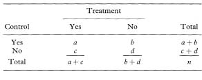
In some crossover or within-person trials the risk difference may be felt to be the appropriate outcome measure. From Table 11.2, the proportions with a good outcome are p_T = (a + c)/n and P_C = (a + b)/n, and thus the relative risk is estimated as R = (a + c) / (a + b).

As with the unpaired case, a confidence interval can be constructed for the logarithm of the relative risk. Væth and Poulsen¹⁴ have shown that the standard error of the log relative risk from paired data is

The 100(1 – α)% confidence interval for log_e R is found by first calculating the quantities

and

As with the unpaired case (chapter 7), the confidence interval for the population relative risk is obtained by taking the antilogs of the values representing the confidence interval for log_e R, namely e^w to e^x.

Worked example

Women requiring oestrogen replacement who had previously experienced skin reactions were randomly allocated to receive either a matrix patch or a reservoir patch for eight weeks followed by the other patch for eight weeks.¹⁵ Seventy-two women completed the study. The numbers discontinuing because of skin irritation are shown in Table 11.3.

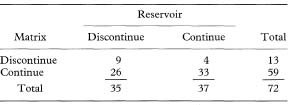
Table 11.3 Numbers of women discontinuing each type of transdermal oestradiol patch because of skin irritation¹⁵

The proportions discontinuing were 13/72 (18%) with the matrix patch and 35/72 (49%) with the reservoir patch, giving an estimated relative risk of R = 13/35 = 0·371. The log relative risk is log_eR = –0·9904. Using the above formula, the standard error of log_e R is

The 95% confidence interval for log_eR is log_eR – 1·96 × 0·2568 to log_e R + 1·96 × 0·2568, or –1·49 to –0·487. The 95% confidence interval for the relative risk R is thus e^–1·49 to e^–0·487, or 0·22 to 0·61.

Multiple groups

Some trials have more than two treatment groups. Confidence intervals can be constructed using the methods given above for any pair of groups. The question of whether to make any allowance for multiple testing is considered in chapter 13.

Subgroups

Comparing P values alone can be misleading. Comparing confidence intervals is less likely to mislead. However, the best approach here is to compare directly the sizes of the treatment effects.¹⁶ When comparing two independent estimates with standard errors (SE₁ and SE₂) we can derive the standard error of the difference very simply as Much the same procedure for comparing subgroups applies to all outcome measures, although the details may vary. (For continuous data we might prefer to use the method based on pooling the standard deviations, as described in chapter 4. It will give very similar answers unless the two standard deviations differ considerably.) A confidence interval can be constructed in the usual way (as described in chapters 4 and 6), using the difference in estimates ± z_{1 – α/2} SE_diff or ± t_{1 – α/2} SE_diff as appropriate.

Table 11.4 Serum calcium levels at one week (mmol/1)

Worked example

In a study of the effect of vitamin D supplementation for the prevention of neonatal hypocalcaemia¹⁷ expectant mothers were given either supplements or placebo and the serum calcium of the baby was measured at one week. The benefit of supplementation was reported separately for breast and bottle-fed infants, and t tests to compare the treatment groups gave P = 0·40 in the breast fed group and P = 0·0006 in the bottle-fed group (Table 11.4). It is wrong to infer that vitamin D supplementation had a different effect on breast- and bottle-fed babies on the basis of these two P values.

The estimated effect of vitamin D supplementation was 0·04 mmol/1 (95% confidence interval –0·07 to +0·15mmol/1) in 166 breast-fed babies and 0·10mmol/1 (95% confidence interval +0·04 to +0·16mmol/1) in 454 bottle-fed babies.¹⁶ The 95% confidence intervals for the two groups thus overlap considerably.

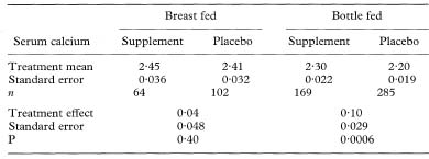
The difference in treatment effects in the two subgroups was 0·10 – 0·04 = 0·06 mmol/1. Using the preceding method, the standard error of this difference is obtained as Because of the large sample size we can use the Normal approximation to the t distribution to calculate a confidence interval. (If we use the t method there are N – 4 degrees of freedom for the t statistic where N is the total trial size.)

The 95% confidence interval for the contrast between the groups is thus 0·06 – 1·96 × 0·0561 to 0·06 + 1·96 × 0·0561, or –0·05 to 0·17 mmol/1. There is thus no good evidence that the effect of vitamin D supplementation differs between breast- and bottle-fed infants.

Table 11.5 Outcomes after intensive insulin treatment versus standard treatment following myocardial infarction²¹

Presentation

There are few problems regarding the presentation of confidence intervals from clinical trials, other than for the NNT as discussed already. One point worth emphasising is that the confidence interval should always be presented for the difference in outcome between the treatment groups. It is a common error to present instead separate confidence intervals for the means or event rates observed in each group. A similar error is to calculate the confidence interval associated with change from baseline in each group. This error has been noted in about 10% of published trials.¹⁸,¹⁹

Confidence intervals are widely used in journals of secondary publication, in which each study is given one journal page which includes both a summary of the paper and a short commentary on it. An example of the style of presentation is given Table 11.5, which summarises the results of a randomised trial comparing intensive versus standard insulin treatment after acute myocardial infarction in diabetics²⁰ as presented in Evidence-Based Medicine.

In recent years many journals have begun to require authors to present confidence intervals in their papers, especially for the principal outcomes. Particular attention has been given to randomised controlled trials, culminating in the CONSORT statement.²² These guidelines, which have been adopted by over 70 journals, include the requirement that authors present confidence intervals. Reporting of results is considered in more depth in chapters 14 and 15.

Interpretation

The interpretation of confidence intervals has been discussed earlier, notably in chapter 3. There should be no special problems relating to trials. Confidence intervals are especially useful in association with trials which have not found a significant treatment benefit, as they indicate a range of possible true effects with which the results are compatible. Given that many trials are too small to have adequate power to detect modest yet clinically valuable benefits,²³ the width of the confidence interval can signal the danger of interpreting “no significant difference” as “no difference”. Sadly, authors sometimes ignore the confidence interval when interpreting their results. For example, Sung et al.²⁴ randomised patients to octreotide infusion or emergency sclerotherapy for acute variceal haemorrhage. They randomised 100 patients despite a power calculation showing that they needed 1800 patients to have reasonable power to detect an improvement in response rate from 85% to 90%. The observed rates of controlled bleeding were 84% in the octreotide group and 90% in the sclerotherapy group. They quoted a confidence interval for the treatment difference as 0 to 19%—it should have been –7% to 19%. More seriously, they drew the unjustified conclusion that “octreotide infusion and sclerotherapy are equally effective in controlling variceal haemorrhage”.

Meta-analysis

Many systematic reviews of the literature include a statistical meta-analysis to combine the results of several similar studies. There is a clear need to present confidence intervals when summarising a body of literature. This section considers metaanalyses of randomised trials. Much the same considerations apply to meta-analyses of other types of study, including epidemiological studies.

I will not describe here methods of performing meta-analysis, but will focus instead on the use of confidence intervals in the display of results.

Analysis

Meta-analysis is a two-stage analysis. For each trial a summary of the treatment effect is calculated and then a weighted average of these estimates is obtained, where the weights relate to the precision of each study’s estimate (effectively, the width of the confidence interval). There are various methods of meta-analysis for both binary and continuous data.^{25, 26} In each case, a confidence interval is obtained from the pooled estimate and its standard error using the general formula given in chapter 3. Confidence intervals feature prominently in the presensation of results of metaanalyses.

For any type of outcome an analysis may used a “fixed” or “random” effects approach. The former considers only the data to hand whereas the latter assumes that the studies are representative of some larger population of trials that might have been performed.^{25, 26} Although in many cases the two methods agree quite closely., the random effects approach gives wider confidence intervals because it allows for an additional element of uncertainty.

Continuous outcome

The principal methods for performing meta-analysis of trials with continuous outcomes are the weighted mean difference and the standardised (weighted) mean difference. These methods yield a mean effect with a standard error, so confidence intervals are easily calculated using the general approach outlined in chapter 3.

Binary outcome

As for single trials, meta-analysis of several similar trials with a binary outcome can be based on the risk difference, the relative risk, or the odds ratio. None can be considered to be the best for all circumstances. The Mantel–Haenszel method is commonly used. It was described in chapter 7 in the context of stratified case-control studies. Although most familiar as a means of combining odds ratios, there are also versions of the Mantel-Haenszel method for obtaining either a pooled relative risk or risk difference.²⁷

Worked example

Figure 11.2 shows the risk ratio associated with coronary artery bypass grafting versus coronary angioplasty and its 95% confidence interval for each trial and for the overall estimate (based on a fixed effect analysis). The four smallest trials have been combined.²⁸ For each trial the risk ratio and 95% confidence interval are shown both numerically and graphically. The size of the black boxes is proportional to the weight given to each trial’s results in the meta-analysis. The diamond represents the overall treatment effect (also shown by the dashed line) and its 95% confidence interval, obtained by combining the results of the eight trials.

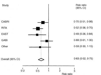
Figure 11.2 Forest plot for meta-analysis of data from eight randomised trials relating to angina in one year comparing coronary artery bypass surgery with coronary angioplasty.²⁸

Outcome is time to an event

Meta-analysis of trials is also possible where the outcome is time to an event. There are serious practical problems, however, as many published papers do not provide the necessary information. Acquiring the raw data from all studies, while desirable, is rarely feasible. Some methods based on published summary statistics have been described by Parmar et al.²⁹

Presentation

Although tables are helpful in meta-analyses, especially to show the actual summary data from each trial, it is usual to show graphically the results of all the trials with their confidence intervals. The most common type of plot is called a forest plot. Such plots tabulate the summary results, estimates and confidence intervals for each study, and depict these graphically. Sometimes the weight given to each trial is also shown. A simplified example is shown in Figure 11.2.

When the effect size has been summarised as relative risk or odds ratio the analysis is based on the logarithms of these values. The forest plot benefits from using a log scale for the treatment effect as the confidence intervals for each trial are then symmetric around the estimate (see Figure 11.2).

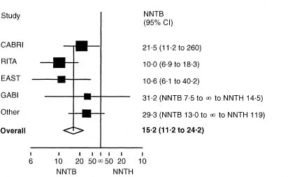
Figure 11.3 Forest plot for the same trials as shown in fig 11.2, showing NNTB for coronary artery bypass surgery and its 95 % confidence interval for each trial and for the overall estimate. The four smallest trials have been combined.

It is common to use 95 % confidence intervals both for each trial and for the overall pooled effect, but some authors use wider confidence intervals (often 99%) for the pooled estimate on the grounds that one is looking for convincing evidence regarding treatment benefit, while others use 99% confidence intervals for the results of each trial.

A forest plot can also be made using the NNT. Noting, as before, that the NNT should be plotted on the absolute risk reduction scale, it is relatively simple to plot NNTs with confidence intervals for multiple trials, even when (as is usual) some of the trials did not show statistically significant results. Figure 11.3 shows such a plot for the same trials as in Figure 11.2. The plot was produced using the absolute risk reduction scale, and then relabelled (this cannot be done in many software packages). Both scales can be shown in the figure.

Interpretation

As already noted, confidence intervals are an especially important feature of meta-analyses. Systematic reviews of the literature aim to provide a reliable answer based on all available evidence. It is important to know not just the average overall effect but also to be able to see how much uncertainty is associated with that estimate.

Software

CIA can perform all of the methods described for randomised controlled trials, but not those for meta-analysis, for which specialist software is advisable.

Comment

I have shown how the analysis of clinical trials, including the calculation of confidence intervals, varies for parallel and crossover trials, corresponding to whether the data are unpaired or paired respectively. Some other trial designs also affect the analysis. This applies in particular to cluster randomised trials, in which patients are randomised in groups, such as those with a particular general practitioner or attending a particular hospital. For such trials analysis of individual patient data is misleading and will lead to confidence intervals which are too narrow. It is essential that the analysis of such trials is based on the randomised clusters.³⁰

Although the focus of interest in this chapter has been on primary treatment effects, there is a similar need to provide confidence intervals for other outcomes, including adverse events and cost data. Such information is usually missing from published reports.³¹

1 Pitt P, Li F, Todd P, Webber D, Pack S, Moniz C. A double blind placebo controlled study to determine the effects of intermittent cyclical etidronate on bone mineral density in patients undergoing long term oral corticosteroid therapy. Thorax 1998;53:351–6.

2 Sackett DL, Deeks JJ, Altman DG. Down with odds ratios! Evidence-Based Med 1996;1:164–6.

3 Rai R, Cohen H, Dave M, Regan L. Randomised controlled trial of aspirin and aspirin plus heparin in pregnant women with recurrent miscarriage associated with phospholipid antibodies (or antiphospholipid antibodies). BMJ 1997; 314:253–7.

4 Senn S. Baselines and covariate information. In: Statistical issues in drug development. Chichester: John Wiley, 1997:95–109.

5 Altman DG. Covariate imbalance, adjustment for. In: Armitage P, Colton T (eds) Encyclopedia of bio statistics. Chichester: John Wiley, 1998: 1000–5.

6 Laupacis A, Sackett DL, Roberts RS. An assessment of clinically useful measures of the consequences of treatment. N Engl J Med 1988;318:1728–33.

7 Cook RJ, Sackett DL. The number needed to treat: a clinically useful measure of treatment effect. BMJ 1995; 310:452–4.

8 McQuay HJ, Moore RA. Using numerical results from systematic reviews in clinical practice. Ann Intern Med 1997; 126:712–20.

9 Sackett DL, Richardson WS, Rosenberg W, Haynes RB. Evidence-based medicine. How to practise and teach EBM. London: Churchill-Livingstone, 1997: 208.

10 Tramèr MR, Moore, RA, Reynolds DJM, McQuay HJ. A quantitative systematic review of ondansetron in treatment of established postoperative nausea and vomiting. BMJ 1997;314:1088–92.

11 Altman DG, Andersen PK. Calculating the number needed to treat for trials where the outcome is time to an event. BMJ 1999; 319:1492–5.

12 Baigent C, Collins R, Appleby P, Parish S, Sleight P, Peto R. ISIS-2: 10 year survival among patients with suspected acute myocardial infarction in randomised comparison of intravenous streptokinase, oral aspirin, both, or neither. BMJ 1998;316:1337–43.

13 Senn S. Cross-over trials in clinical research. Chichester: John Wiley, 1993.

14 Væth M, Poulsen S. Comments on a commentary: statistical evaluation of split mouth caries trials. Community Dent Oral Epidemiol 1998;26:80–3.

15 Ross D, Rees M, Godfree V, Cooper A, Hart D, Kingland C, Whitehead M. Randomised crossover comparison of skin irritation with two transdermal oestradiol patches. BMJ 1997;317:288.

16 Matthews JNS, Altman DG. Interaction 3: How to examine heterogeneity. BMJ 1996;313:862.

17 Cockbum F, Belton NR, Purvis RJ, Giles MM, et al. Maternal vitamin D intake and mineral metabolism in mothers and their newborn infants. BMJ 1980;281:11–14.

18 Altman DG, Doré CJ. Randomisation and baseline comparisons in clinical trials. Lancet 1990;335:149–53.

19 Gøtzsche PC. Methodology and overt and hidden bias in reports of 196 doubleblind trials of non-steroidal antiinflammatory drugs in rheumatoid arthritis. Controlled Clin Trials 1989;10:31–56.

20 Malmberg K for the DIGAMI Study Group. Prospective randomised study of intensive insulin treatment on long term survival after acute myocardial infarction in patients with diabetes mellitus. BMJ 1997;314:1512–15.

21 Malmberg K for the DIGAMI Study Group. Intensive insulin regimen reduced long-term mortality after MI in diabetes mellitus. Evidence-Based Med 1997;2:173.

22 Begg C, Cho M, Eastwood S, Horton R, Moher D, Olkin I, et al. Improving the quality of reporting of randomized controlled trials: the CONSORT statement. JAMA 1996;276:637–9.

23 Thornley B, Adams C. Content and quality of 2000 controlled trials in schizophrenia over 50 years. BMJ 1998;317:1181–4.

24 Sung JJY, Chung SCS, Lai C-W, Chan FKL, et al. Octreotide infusion or emergency sclerotherapy for variceal haemorrhage. Lancet 1993;342:637– 41.

25 Fleiss JL. The statistical basis of meta-analysis. Stat Meth Med Res 1993;2:121– 45.

26 DerSimonian R, Laird N. Meta-analysis in clinical trials. Controlled Clin Trials 1986;7:177–86.

27 Greenland S, Robins J. Estimation of a common effect parameter from sparse follow-up data. Biometrics 1985;41;55–68.

28 Pocock SJ, Henderson RA, Rickards AF, Hampton JR, King SB, Hamm CW et al. Meta-analysis of randomised trials comparing coronary angioplasty with bypass surgery. Lancet 1995;346:1184–9.

29 Parmar M, Torri V, Stewart L. Extracting summary statistics to perform metaanalyses of the published literature for survival endpoints. Stat Med 1998;117:2815–34.

30 Kerry SM, Bland JM. Analysis of a trial randomised in clusters. BMJ 1998;316:54.

31 Barber JA, Thompson SG. Analysis and interpretation of cost data in randomised controlled trials: review of published studies. BMJ 1998;317:1195–200.