CHAPTER 8

FOURIER TRANSFORMS

8.1 FOURIER INTEGRALS

In previous chapters, all of the partial differential equations we studied were defined on a finite domain [a, b], and the differential operators we obtained by separating variables had a discrete spectrum. In this case, the solution could be represented as an infinite series of orthogonal eigenfunctions.

In this chapter we study partial differential equations defined on an infinite domain, either (0, ∞), or (–∞, ∞), and usually the differential operators do not have a discrete spectrum. In this case, instead of getting a representation for solutions on a finite domain [a, b] in terms of generalized Fourier series, we get a representation on (0, ∞) or (–∞, ∞) in terms of improper integrals, called Fourier integrals.

8.1.1 Fourier Integral Representation

In this section we give a heuristic argument for the Fourier integral formula: Assuming that f is defined for all real numbers x, that both f and f′ are piecewise continuous

on every finite interval [–a, a], and that f is absolutely integrable on , that is,

f can be represented by its Fourier integral

where

for ω > 0. Note that since f is absolutely integrable, both of these integrals converge.

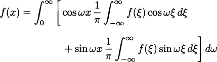
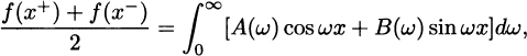
As with Fourier series, before we can determine the convergence of the integrals, we write

where A(ω) and B(ω) are as given above. This is called the Fourier integral formula for f(x) on the interval – ∞ < x < ∞. To show why this might be true, we assume that f(x) is actually continuous on every finite interval and that f′(x) is piecewise continuous. Then f(x) has a Fourier series expansion on [–a, a], and by Dirichlet’s theorem we can write

for –a < x < a, where

for n ≥ 1. Now we define ω_n = nπ/a, and rewrite the coefficients as

where

for n ≥ 1.

The formula for the Fourier series becomes

that is,

(8.1)

where for n ≥ 1. Now, as a → ∞ we have Δω_n → 0 and ω₁ → 0, and since

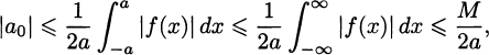
where M is a constant, a₀ → 0 as a → ∞. The series resembles a limit of Riemann sums:

(8.2)

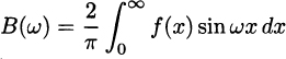
where

that is,

for 0 < ω < ∞. A rigorous proof of the Fourier integral formulas (8.2) and (8.3) requires a careful study of the limits involved, and will be given in Section 8.1.4.

In the case where f is not continuous everywhere on but is piecewise continuous on every finite interval, then according to Dirichlet’s theorem, we would expect that

(8.4)

for –∞ < x < ∞.

The formula (8.4) is called the Fourier integral representation of the function f(x), while A(ω) and B(ω) are called the Fourier integral coefficients of f. Note that if f is continuous at x, (8.4) becomes (8.2). We have the following convergence theorem, similar to Dirichlet’s theorem for Fourier series.

Theorem 8.1. (Fourier Integral Theorem)

If f and f′ are piecewise continuous on every finite interval [a, b] ⊂ and f is absolutely integrable on , that is,

the Fourier integral

where

for 0 < ω < ∞, converges to

at each point x ∈ .

8.1.2 Examples

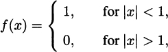
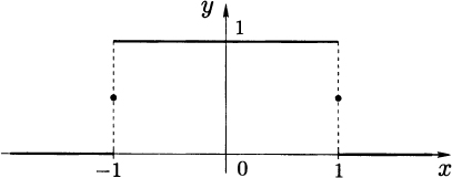
Example 8.1. Given the rectangular pulse

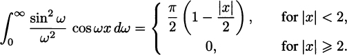
and f(l) = f(–1) = . Show that the Fourier integral formula for f is

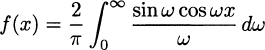
for all x ∈ .

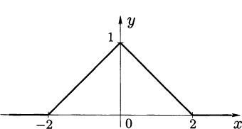
Solution. The graph of the rectangular pulse is shown in Figure 8.1. Clearly, the function f is piecewise smooth on , and

Figure 8.1 Rectangular pulse,

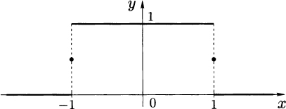
so the conditions for Dirichlet’s theorem hold. Now,

for 0 < ω < ∞, and

for 0 < ω < ∞. From Dirichlet’s theorem we have

for all x ∈ , and hence

This integral is called Dirichlet’s discontinuous factor.

In particular, for x = 0, since f(0) = 1, we have

thus, the integral converges, even though, as we show later in Lemma 8.4,

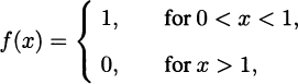
Example 8.2. Find the Fourier integral representation of the function

and f(0) =

Solution. The graph of the function f(x) is shown in Figure 8.2. Again, it is clear that the function f is piecewise smooth on , and

so the conditions for Dirichlet’s theorem hold. Now

Therefore,

so that

that is,

Figure 8.2 Exponential pulse.

and

for 0 < ω < ∞. Also,

and

for 0 < ω < ∞. Thus,

for all x ∈ .

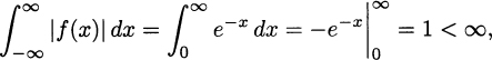
Example 8.3. Calculate the Fourier integral of the function

Solution. Clearly, f is piecewise continuous on (–∞, ∞); is absolutely integrable, since

and hence f satisfies the hypotheses of Dirichlet’s theorem. Computing the Fourier integral coefficients, we have

and since f(x) is even, then

Therefore,

for all x ∈ (–∞, ∞).

8.1.3 Fourier Sine and Cosine Integral Representations

From Examples 8.1 and 8.3, the Fourier integral of an even function contained only cosine terms, just as with Fourier series; similarly, the Fourier integral of an odd function will contain only sine terms. If the function f is defined on the interval (–∞, ∞), the Fourier integral coefficients A(ω) and B(ω) are uniquely determined, and the Fourier integral representation for f on may contain both sine and cosine terms. However, on infinite domains, the PDEs we solve using separation of variables typically have either no boundary conditions or boundary conditions specified on the subinterval (0, ∞) and usually lead to integrals containing only sine terms or to integrals containing only cosine terms. If the function f is defined only on the interval (0, ∞), we may extend it to the interval (–∞, ∞) either as an odd function f odd or as an even function f_even. From the previous remarks, the Fourier integral for f_odd on the interval (–∞, ∞) contains only sine terms, while the Fourier integral for f_even on the interval (–∞, ∞) contains only cosine terms. Both f_odd and f_eVen agree with f on the interval (0, ∞); hence, f has two different Fourier integral representations on the interval (0, ∞).

Definition 8.2. Suppose that f is defined on (0, ∞) and is absolutely integrable there, that is,

then:

(i) the Fourier cosine integral for f on (0, ∞) is

where

for 0 < ω < ∞, and

(ii) the Fourier sine integral for f on (0, ∞) is

where

for 0 < ω < ∞.

We have a result similar to Dirichlet’s convergence theorem for the Fourier sine and cosine integrals, and it follows immediately from the Fourier integral theorem.

Theorem 8.3. If f is defined on the interval (0, ∞), f and f′ are piecewise continuous on every finite subinterval of (0, ∞), and f is absolutely integrable on (0, ∞), then the following are true:

(i) For the Fourier cosine integral,

where

for 0 < ω < ∞.

(ii) For the Fourier sine integral,

where

for 0 < ω < ∞,

Example 8.4. Find the Fourier cosine and sine integral formulas for

and f(0) = 1, f(l) = .

Figure 8.3 Even extension.

Solution

• For the Fourier cosine integral, the graph of the even extension (Fig. 8.3) is the same as the graph in Example 8.1. Here,

thus, the Fourier cosine integral of f is

• For the Fourier sine integral, the graph of the odd extension of f is shown in Figure 8.4. Here,

Figure 8.4 Odd extension.

thus, the Fourier sine integral of f is

that is,

8.1.4 Proof of Fourier’s Theorem

We begin by giving an elementary proof of the following lemma.

Lemma 8.4. (Dirichlet’s Integral)

Proof. The following proof is outlined on page 397, Miscellaneous Exercise 39, in G. H. Hardy’s A Course of Pure Mathematics [26].

(a) For each n ≥ 1, define

and consider the difference u_n+1 – u_n,

therefore, u_n+1 – u_n = 0 for all n ≥ 1. Thus, u_n is constant for n ≥ 1, and

and therefore u_n = u₁ = π/2 for all n ≥ 1.

Making the substitution t = 2nx in the integral , then

(8.5)

and integrating by parts, we have

and therefore

Using L’Hospital’s rule, we have

Therefore, we may redefine the integrand on the right-hand side of (8.6) to be continuous on the interval [0, π/2], and hence bounded there. Thus, there exists a constant M > 0 such that

Letting n → ∞ in (8.5) and (8.6), we obtain

so that

(b) For each positive integer n, we have

where the last equality follows since sin t ≥ 0 for 0 ≤ t ≤ π. For 0 < t < π, we have 1 /(t + kπ) > l/[π(k + 1)], so that

Now, for x ≥ 1 we have

and replacing x by (k + 2)/(k + 1), we have

for all k ≥ 0. Therefore,

so

and this implies that

The following two lemmas are key to the proof of the Fourier integral theorem.

Lemma 8.5. If f is piecewise continuous on an interval (a, b), then

for all x ∈ (a, b).

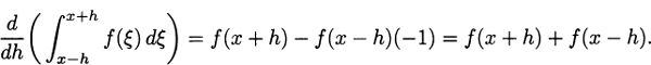
Proof. If x ∈ (a, b) and f is continuous at x, since f is piecewise continuous on (a, b), we can choose h > 0 so small that f is continuous on the interval (x – 2h, x + 2h). Writing

from the fundamental theorem of calculus, we have

From L’Hospital’s rule, since f(x⁺) and f(x^–) both exist, we have

If f has a jump discontinuity at x, again since f is piecewise continuous on (a, b), we can choose h > 0 so small that f is continuous on the interval (x – 2h, x) and also on the interval (x, x + 2h). Now the same argument given above works.

Lemma 8.6.

Proof. If ξ = 0, the result is obvious. If ξ > 0, making the change of variable x = ωξ then

On the other hand, if ξ < 0, making the change of variable x = –ωξ then

Now, for real numbers x and h, we define

and note that K is an even function of x. We have

Using Lemma 8.6, we have

and therefore

that is,

Finally, we can prove Theorem 8.1.

Theorem 8.7. (Fourier Integral Theorem)

If f and f′ are piecewise continuous on every interval (a, b), and f is absolutely integrable on (–∞, ∞), that is,

the Fourier integral

where

for 0 < ω < ∞, converges to

at each point x ∈ .

Proof. From Lemma 8.5 and the definition of K(x, h), we have

Interchanging the limit and integration processes yields

Finally, interchanging the order of integration, we have

that is,

from the definition of the Fourier integral coefficients.

8.2 FOURIER TRANSFORMS

In this section we give the definitions and basic properties of the Fourier transform. Assuming that f is defined for all real numbers x, that f is continuous on , that f′ is piecewise continuous on every finite interval (a, b), and that f is absolutely integrable on , that is,

then by Dirichlet’s theorem, f can be represented by the Fourier integral formula

(8.7)

where

for ω > 0. Thus,

that is

for –∞ < x < ∞. Note that

is an even function of ω, so that

and thus,

(8.8)

Note also that

is an odd function of ω, so that

and thus

Therefore,

and we rewrite this last equality as

(8.9)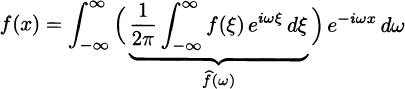

for –∞ < x < ∞. Note that if f has a jump discontinuity at x₀ ∈ , then from Dirichlet’s theorem we have

(8.10)

Definition 8.8. If f is piecewise smooth on every finite interval (a, b) and

the Fourier transform of f(x) is

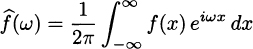
for –∞ < x < ∞.

Using (8.9) and (8.10), we can restate Theorem 8.1 in terms of Fourier transforms.

Theorem 8.9. If f and f′ are piecewise continuous on every finite interval (a, b) and f is absolutely integrable on (–∞, ∞), then

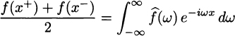
for –∞ < x < ∞.

Definition 8.10. If f is piecewise smooth on every finite interval (a, b) and absolutely integrable on (–∞, ∞), then

(8.12)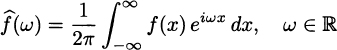

and

(8.13)

form what is called a Fourier transform pair.

Definition 8.11. If f is piecewise smooth on every finite interval (a, b), absolutely integrable on (–∞, ∞) and f is continuous on (–∞, ∞), then

(8.14)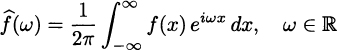

and

(8.15)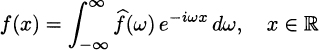

and f(x) is called the inverse Fourier transform of

Notation: For the Fourier transform and the inverse Fourier transform we have:

• The Fourier transform of f is sometimes denoted by

and

• the inverse Fourier transform of is sometimes denoted by

or any combination thereof. The reader is cautioned that there is no standard definition of the Fourier transform and the inverse Fourier transform. Hence, in some textbooks you will find the Fourier transform and the inverse Fourier transform with different factors in front and/or different signs in the exponent. We will be consistent throughout this book and use the notation presented in the preceding definitions.

Example 8.5. In this example we find the Fourier transform pair for f(x) = e^–|x|, Clearly, f satisfies the hypothesis of the Fourier integral theorem, and

Therefore,

8.2.1 Operational Properties of the Fourier Transform

In the next few theorems, we show that the Fourier transform and the inverse Fourier transform are linear operators, and state the shift theorems and the dilation theorem for the Fourier transform. We will need these results in Chapter 9 when we use transform methods to solve PDEs,

Theorem 8.12. (Linearity)

(a) If f and g are piecewise smooth on every finite interval, and absolutely integrable on , then

(b) If, in addition, f and g are continuous on , then

Proof. We will give the proof for the Fourier transform; the proof for the inverse transform is exactly the same.

for –∞ < ω < ∞.

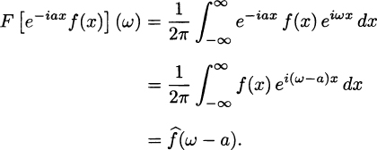
Theorem 8.13. (Shift Theorems)

If f is piecewise continuous on every finite interval and is absolutely integrable on , and a ≠ 0 is a real number, then

for –∞ < ω < ∞.

Proof. Suppose that f is piecewise smooth on every finite interval and is absolutely integrable on .

(a) From the definition of the Fourier transform, we have

(b) Again, from the definition we have

We leave the proof of (c) as an exercise.

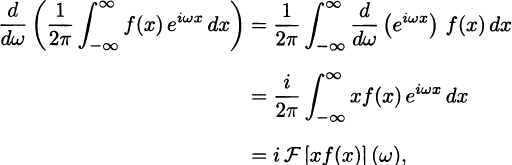
Now we indicate the relationship between the Fourier transform operator and the operations of differentiation and integration.

Theorem 8.14. (Transforms of Derivatives)

If f is piecewise smooth, f and f′ are integrable, and f(x) → 0 as |x| → ∞, then

(b) If f′ is piecewise smooth, f″ is integrable, and f′(x) → 0 as |x| → ∞, then

(c) In general, if f and f^(k), for k = 1, 2, …, n – 1, are piecewise smooth and approach 0 as |x| → ω, and f, f′, …, f⁽ⁿ⁾ are integrable, then

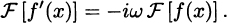
Proof. We will prove part (a); the proofs of (b) and (c) are left as an exercise,

(a) Integrate by parts and use the fact that f(x) → 0 as |x| → ω; then

and therefore

Theorem 8.15. (Transform of an Integral)

If f is continuous on (–∞, ∞), f′ is piecewise continuous on every finite interval (a, b), and f is absolutely integrable on (–∞, ∞), then

for –∞ < ω < ∞.

Proof. Using Theorem 8.14, from the fundamental theorem of calculus we have

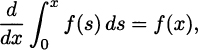
and the result follows.

Theorem 8.16. (Derivatives of Transforms)

Suppose that f is piecewise smooth on every finite interval (a, b).

(a) If f(x) and xf(x) are absolutely integrable on (–∞, ∞), then

(b) If f(x) and xⁿf(x) are integrable, then

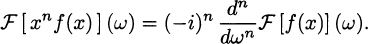
Proof. We give the proof for part (a) and leave the proof for part (b) as an exercise,

(a) We have

and therefore

for –∞ < ω < ∞.

8.2.2 Fourier Sine and Cosine Transforms

In this section we give the definitions and basic properties of the Fourier sine and cosine transforms. Given a function f defined on the semi-infinite domain [0, ∞), we can extend f to as an odd function f_odd, or as an even function f_even, and hence f can have two Fourier transforms:

and

called the Fourier sine transform and the Fourier cosine transform, respectively.

• Fourier Sine Transform

Let f_odd be the odd extension of f to (–∞, ∞), as in Figure 8.5. The Fourier transform of f_odd is

and since f_odd is an odd function, then

Now, f_odd = f on [0, ∞), and hence

for –∞ < ω < ∞. Note that this is an odd function of ω.

Figure 8.5 Odd extension.

The inverse Fourier transform of _odd is

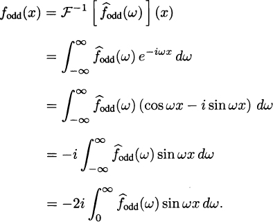
However, f_odd (x) = f(x) for x ∈ [0, ∞), so that

Therefore, if f : [0, ∞) → is extended as an odd function, we have

(8.16)

for 0 < x < ∞; note that (8.16) is just the Fourier sine integral formula.

• Fourier Cosine Transform

Let f_even be the even extension of f to (–∞, ∞), as in Figure 8.6. The Fourier transform of f_even is

and since f_even is an even function, then

Figure 8.6 Even extension.

Now, f_even = f on [0, ∞), and hence

for –∞ < ω < ∞. Note that this is an even function of ω. The inverse Fourier transform of _even is

However, f_even(x) = for x ∈ [0, ∞), so that

Therefore, if f : [0, ∞) → is extended as an even function, we have

(8.17)

for 0 < x < ∞; and note that (8.17) is just the Fourier cosine integral formula.

Definition 8.17. Let f : [0, ∞) → be continuous and absolutely integrable on (0, ∞), and let f′ be piecewise continuous on every finite interval (a, b) ⊂ (0, ∞). Then the sine and cosine transform and inverse transform are given by:

(i) The Fourier sine transform of f(x) is

and the inverse sine transform of g(ω) is

(ii) The Fourier cosine transform of f(x) is

and the inverse cosine transform of g(ω) is

Note: From the definitions above and Dirichlet’s theorem, we have

(i) , that is,

for 0 < x < ∞.

(ii) , that is,

for 0 < x < ∞.

8.2.3 Operational Properties of the Fourier Sine and Cosine Transforms

The linearity of the sine and cosine transforms is evident; we only give the results on transforms of derivatives here.

Theorem 8.18. (Transforms of Derivatives)

If f is piecewise smooth, f and f′ are integrable on [0, ∞), and lim _x→∞ f(x) → 0, then:

(a) For the Fourier sine transform, we have

and if f″ is integrable on [0, ∞) and lim _x→∞ f′(x) also, then

(b) For the Fourier cosine transform, we have

and if f″ is integrable on [0, ∞) and lim _x→∞ f′(x) also, then

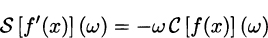
Proof. We give the proof of the first part of (a); proofs of the remaining results are left as an exercise.

(a) Integrating by parts gives

and since f(x) → 0 as x → ∞, then

Note: From Theorem 8.18, it is obvious that the following are true:

(i) If the Fourier sine transform is used to solve a PDE, then f(0); that is, u(0, t) must be known, for example, a Dirichlet boundary condition at x = 0.

(ii) If the Fourier cosine transform is used to solve a PDE, then f′(0); that is, ∂u(0, t)/∂x, must be known, for example, a Neumann boundary condition at x = 0.

8.2.4 Fourier Transforms and Convolutions

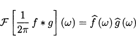
When solving PDEs using Fourier transforms, one is faced with the problem of having to find the inverse Fourier transform of a product of the form F(ω) · G(ω), where F and G are, respectively, the Fourier transforms of the functions f and g. Unfortunately, the inverse Fourier transform of the product is not the product of the inverse Fourier transforms. To find the inverse Fourier transform of a product, we need to introduce the convolution of two functions.

Definition 8.19. (Convolution Product)

If f and g are defined on all of , and are integrable over , the convolution of f and g is given by

for –∞ < x < ∞.

The following lemma lists some of the properties satisfied by the convolution.

Lemma 8.20. (Properties of the Convolution)

Suppose that a ∈ and that f, g, h are integrable over , then

(a) f * g = g * f,

(b) a(f * g) = (af) * g = f * (ag),

(c) (f * g) * h = f * (g * h),

(d) f * (g + h) = f * g + f * h.

Proof. We will prove (a) and leave the rest as an exercise,

(a) If f and g are integrable over , then

for all x ∈ .

Example 8.6. (Convolution with a Sine)

Let f be an even integrable function on , and let g(x) = sin ax for x ∈ , where a > 0 is constant; then

where is the Fourier transform of f. Solution. We have

and since f is even,

And, again, since f is even,

Theorem 8.21. (Convolution Theorem)

If f and g are integrable and satisfy the hypotheses of Dirichlet’s theorem, that is, the Fourier integral theorem, then

(a)

(b) If, in addition, f and g are continuous, then

Proof. For part (a), we have

and letting u = x – t yields

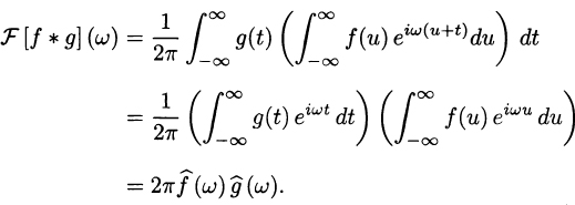
Therefore,

for – ∞ < ω < ∞. The proof of part (b) follows from the definition of the inverse Fourier transform.

Example 8.7. Find the Fourier transform of the function

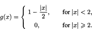
Solution. The graph of g is shown in Figure 8.7. Clearly, g and g′ are piecewise

Figure 8.7 Tent function g(x).

continuous on , and

thus, g satisfies the hypotheses of the Fourier integral theorem (i.e., Dirichlet’s theorem), and therefore, for ω ≠ 0,

since g(x) is an even function. Therefore, for ω ≠ 0, we have

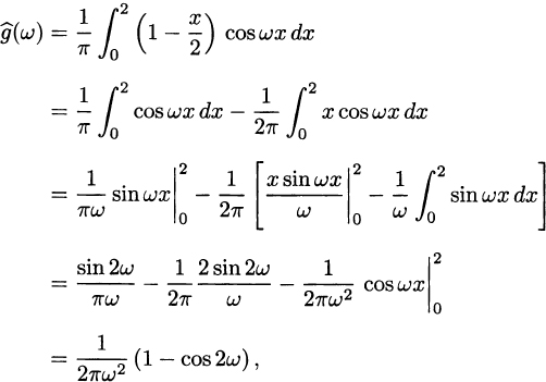
and thus,

For ω = 0, we have

Note that

and is continuous at all ω ∈

In fact, the next result shows that this is true in general (we omit the proof).

Theorem 8.22. If the function f : → is piecewise smooth on every finite interval and is absolutely integrable on , that is,

then the Fourier transform

is uniformly continuous on .

Example 8.8. Let f(x) be the rectangular pulse

and whose graph is shown in Figure 8.8 Let h(x) be the convolution of f with itself, that is,

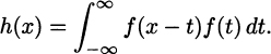
Find the Fourier transform of h(x), and use the convolution theorem to identify h(x).

Solution. First we find the Fourier transform of f(x); for ω ≡ 0 we have

Figure 8.8 Rectangular pulse.

while for ω = 0, we have

Now, the Fourier transform of h(x) = (f*f) (x) is given by

for ω ≠ 0, and (0) = 2/π. Therefore,

where (ω) was found in Example 8.7. Thus,

Note: This can be used to evaluate certain improper integrals. For example, from the above we have

and therefore

8.2.5 Fourier Transform of a Gaussian Function

In the next chapter we solve the problem of heat conduction in an unbounded region, first for an infinite rod, where there are no boundary conditions, and next for a semi-infinite rod, where there is one boundary condition. In the first case we use the Fourier transform. In the second case we use either the Fourier sine transform or the Fourier cosine transform, depending, respectively, on whether the one boundary condition is a Dirichlet condition or a Neumann condition. We will need the following integrals.

Lemma 8.23. If b > 0, then

Proof. We write

so that

Introducing polar coordinates ρ and θ, we have

and

Lemma 8.24. If b > 0, then

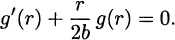
for all real numbers r.

Proof. Let b > 0 and define the function g by

for – ∞ < r < ∞. Since the improper integral converges uniformly on every finite interval and the integral

converges uniformly on every finite interval, g is differentiable. Differentiating under the integral sign, and then integrating by parts, we have

and g(r) satisfies the first-order linear differential equation

Multiplying by the integrating factor , we have

so that

for – ∞ < r < ∞, where C is constant. The constant of integration is given by

and from Lemma 8.23, we have

for –∞ < r < ∞.

Now we prove the important result that the Fourier transform of a Gaussian function is again a Gaussian function (to within a multiplicative constant).

Theorem 8.25. (Fourier Transform of a Gaussian Function)

Let a > 0 be an arbitrary constant; then

Proof. Let (ω) be the Fourier transform of the function

that is,

for –∞ < ω < ∞; then

for –∞ < ω < ∞. Since e^–ax2 is an even function, then from Lemma 8.24 we have

for –∞ < ω < ∞.

Corollary 8.26. Let a > 0 be an arbitrary constant; then

for –∞ < x < ∞.

Proof. This follows from Theorems 8.7 and 8.25.

8.3 SUMMARY

In Chapter 2 on Fourier series, we defined the Fourier series for functions in PWC(–, ), and the Fourier sine series and Fourier cosine series for functions in PWC(0, ). Thus, Fourier series are used on symmetric domains (–, ), while Fourier sine series and Fourier cosine series are used on the domain [0, ). The situation is similar here: The Fourier transform is applied to problems on (–∞, ∞), while the Fourier sine transform and Fourier cosiiie transform are appled to problems on (0, ). The Fourier transform can be written as an integral transform

and the inverse Fourier transform as

In using the Fourier transform, we enter a new world, the ω-world. In physical applications, the ω-world is also called the frequency domain, and indeed, local peaks of the Fourier transform correspond to dominant frequencies of the original function.

The Fourier sine and cosine transforms apply to functions defined on (0, ∞) and are closely related to the Fourier transform, and as such, they have very similar properties. We give several detailed examples in the text.

8.3.1 Problems and Notes

Problems from Part II:

Final exam questions:

Exercise	19.1	19.10
Notes

You should now be able to do Final Exams 1 and 3.