Google Cloud Logging, known until March 2020 as Stackdriver, is the central tool used to collect event logs from all of your systems. As with other systems we’ve discussed, it is fully managed and supports event collection at scale. It’s also directly integrated with all of the other services we’ve engaged with up until now: BigQuery, Cloud Storage, Cloud Functions, and so forth.
In this chapter, we’ll look at how to import and analyze Cloud Logging logs in BigQuery and how to tie them together to gain system-wide understanding of how your applications are operating. On the flip side of this coin, BigQuery generates logs to Cloud Logging itself, which you can also import back into BigQuery for analysis.
All of this is building up to advanced topics in Parts 4 and 5, where we’ll get into the long-term potential of the data warehouse using reporting, visualization, and real-time dashboarding. Adding performance monitoring to this mix is a surefire way to vault you ahead of your competition.
How This Is Related
What does logging have to do with data analysis or data warehouses? Why is it important for us to be familiar with how it works? One modern paradigm in DevOps is remaining cognizant of the fact that monitoring an application is closely related to monitoring what users do with an application. Detecting normal user activity, elevated error rates, unauthorized intrusions, and reviewing application logs all share some similarities.
BigQuery enters the picture as a tool for analyzing these massive amounts of real-time data over much longer periods of time and with the ability to regard Cloud Logging as only a single facet of the available data. To go all the way up the ladder again, the idea is to create insights from information from data. Simultaneously, you can analyze application-level inputs and outputs, what effect those are having on the overall system, how healthy the system is, how much it is costing you, and if it is being used as expected. Until now, it would have been difficult to get so close to the real-time unit economics of every single event on your business. Let me illustrate a little more concretely with concepts we’ll cover as we go through this chapter.
An Example: Abigail’s Flowers
Abigail’s Flowers (AF) is a successful ecommerce business that ships customized floral bouquets ordered through their website. BigQuery is already a fixture in the business, powering all of their analytics dashboards and providing real-time insight into current orders. They even have a small predictive function that allows them to forecast impending demand. How can Cloud Logging help in such a sophisticated business?
Ensure the application is recording the results of payment calls. It turns out that it’s already doing this through a Cloud Logging event.
The team creates an event sink to BigQuery for these calls and lets it run for a few hours.
Meanwhile, they ensure that the payment API itself is recording its requests and responses. This is also already being logged to Cloud Logging.
They make an event sink for the payment API as well.
The team also looks more closely at application performance using Cloud Monitoring. There are no unusual spikes or long-running calls, so they rule out slowness and timeouts as a root cause. (They make a sink anyway, just in case.)
Lastly, they review their BigQuery schemas and learn where data about user accounts and user orders is being logged.
Now they have two important types of data: the performance of the application and the behavior of the application in use. The team starts their analysis.
When do payment failures occur? Are they higher by day of the week and/or hour of the day? (Remember, this number wasn’t significant across all errors on the system, but it may be visible when looking solely at payment errors.)
What kinds of errors are occurring in payment? Do they happen on the application or in the API?
How many orders are being made when the error rate is higher?
How many distinct users are making orders when the error rate is higher?
What are the characteristics of users with high numbers of failing orders?
What are the characteristics of orders that are failing?
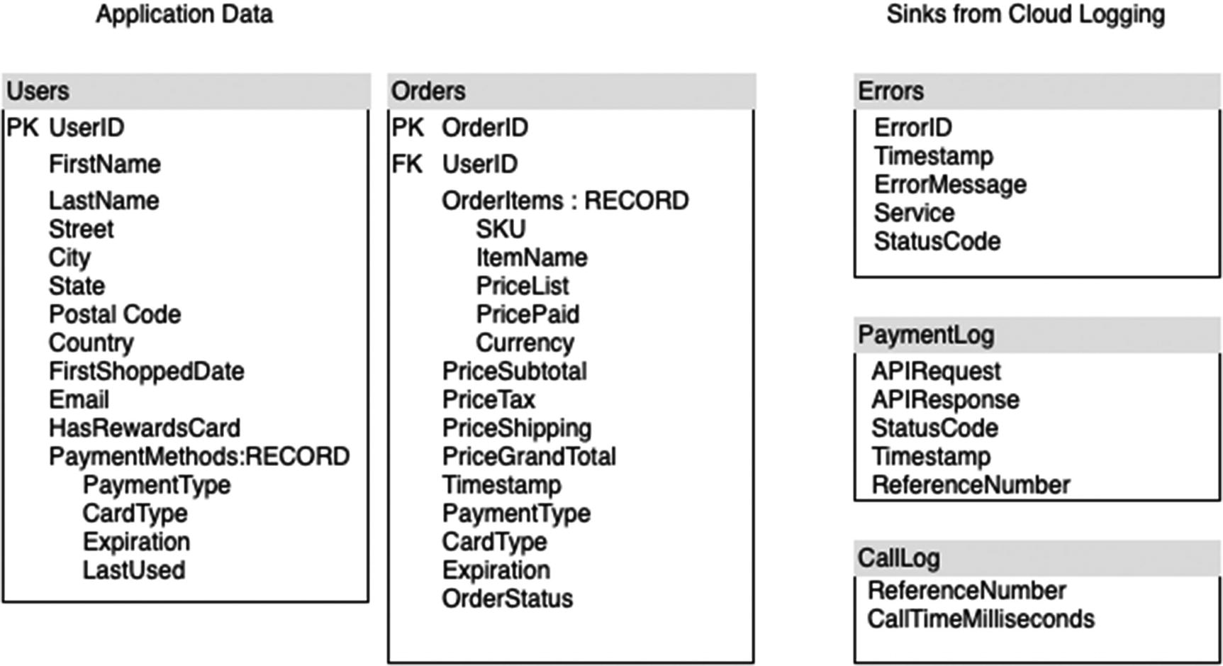
The data schema for Abigail’s Flowers
Note that BigQuery doesn’t actually have the concept of primary and foreign keys; these are just used to illustrate the logical data relations.
This information is only accessible to them because they have both the error information and the account/order information in BigQuery. If they were in separate data sources, the team would have to export each set of data and merge it manually. There might be manual data transformation errors. Also, there are millions of rows and gigabytes of data in each set, limiting the effectiveness of what can be exported. Even more interestingly, they can now create real-time dashboards that answer these questions as orders come in.
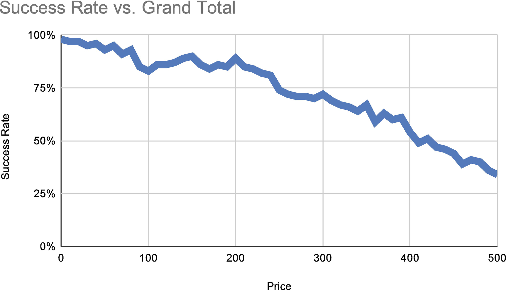
Graph showing correlation between failure rate and price
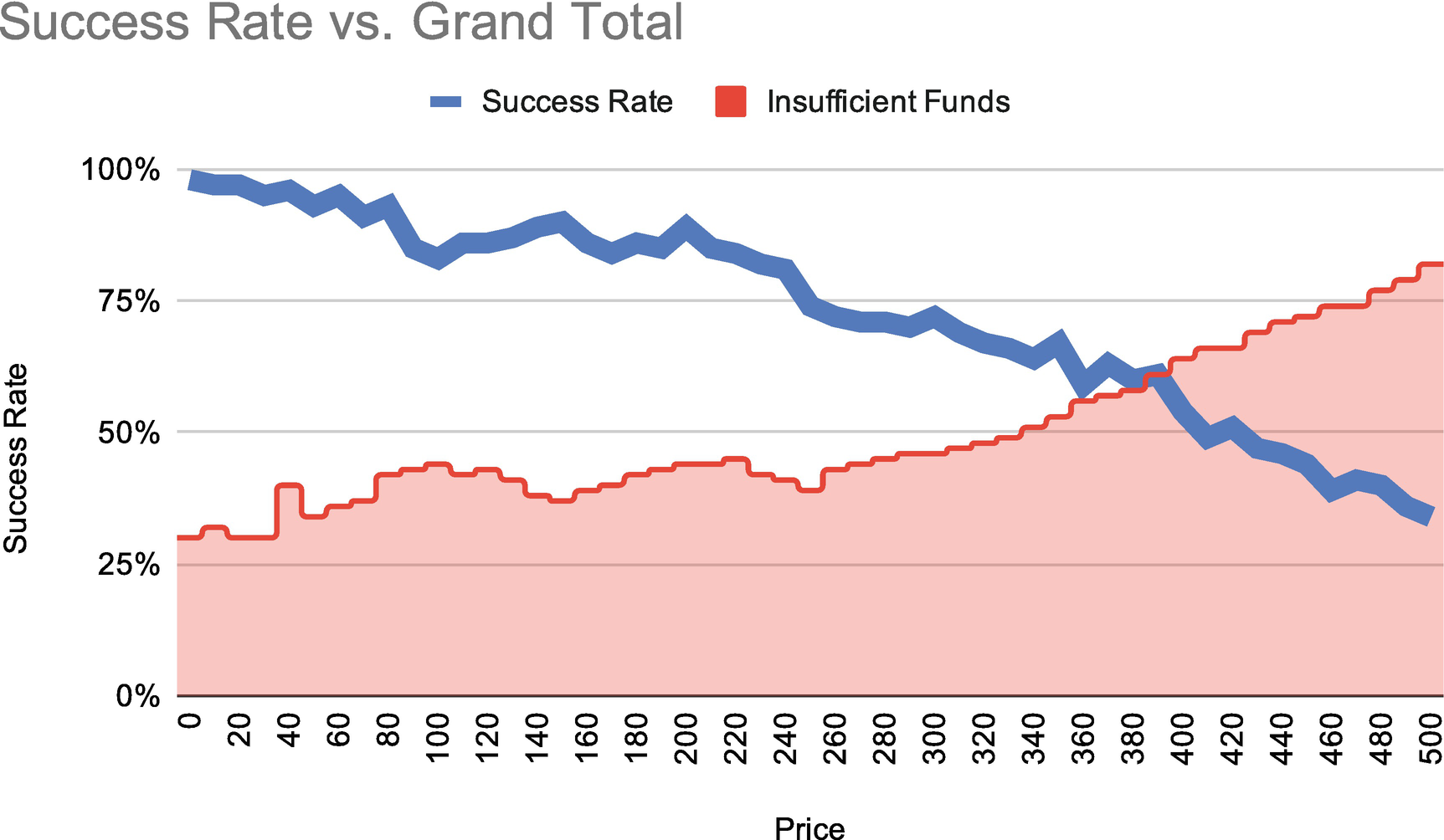
Same graph with error type included
Now it’s crystal clear: this elevated error rate is caused by an error saying that the bank declined the card for insufficient funds. As customers try to charge cards for higher and higher dollar amounts, they are more likely to be declined for this reason. It turns out there’s no problem at all. The issue is caused by customers trying to exceed their credit limits. Relieved, the team leaves the new event sinks in place, creates some additional alerting to fire if this expectation is violated, and goes off to happy hour.
It’s easy to see how this might have spiraled out of control in a less sophisticated organization. Pulling these datasets manually from multiple systems and consolidating them would lead to hours of work to look at a single static view. An inconsistent data warehouse might have made it prohibitively difficult to marry the error logs and the user account data. And as the team was analyzing increasingly stale data, they would have been unable to defend or explain new cases still arriving from customers.
This is a key insight for any business process. Shortening your feedback loop allows you to surface and react to relevant information as soon as it’s generated. Now that the team knows this could be an issue, they can monitor it continuously—and should a cluster of customers report the issue again, they can quickly determine if it has the same root cause or if a new issue has surfaced.
Using this as a template, you can easily imagine constructing more sophisticated scenarios. A live clickstream could be integrated to show how users react to unexpected conditions during payment and used to improve the website experience. An alert could be set on one customer receiving large amounts of errors from many different credit cards, indicating potentially fraudulent transactions. You could see if users who experience these errors are likely to succeed at purchasing on another card or at a later time. Or you could just see if users who encounter errors on one order are more or less likely to become repeat purchasers. These are all ways you might fruitfully integrate Cloud Logging with BigQuery (or, generically, application performance monitoring with your data warehouse tool.)
The Cloud Logging Console
Click the hamburger menu and go to the Logging tab. (Again, if you’ve done this in the past, it was called Stackdriver, but has been renamed. Google likes to rename services on a regular basis to make useful books go out of date.) After a bit, it should bring you to the primary screen, which is the Logs Viewer.
Depending on how much you’ve used Google Cloud Platform to this point, you may not have much to look at yet. By default, it will automatically show all of the services you currently use. Pretty much everything you do on Google Cloud Platform is logged here in excruciating detail. This means it’s very easy to get some data for us to look at in the logs. If you don’t have anything interesting yet, go over to the BigQuery console and do a few select statements from your tables or just select static data. Then come back here.
Looking at Logs
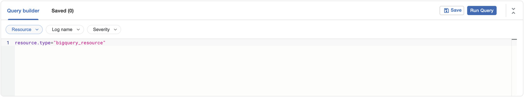
Logging/BigQuery log query panel
Click “Run Query,” and you will see your results populate. This will restrict the view just to events generated by BigQuery. The view is also close to real-time; if you continue performing activity in BigQuery, you can click the “Jump to Now” button to update the results with the latest.
The first thing you will notice here is that there is a tremendous amount of data being logged. Each service has a set of payloads that it uses when recording logs. You can also define your own logging schemas to be emitted from your own services, as we’ll discuss a little later on.
In a way, BigQuery and Cloud Logging have a lot in common. Both can ingest large amounts of data at sub-second latency and make it available for detailed analysis. The biggest difference is that Cloud Logging data is inherently ephemeral. It’s designed to collect all the telemetry you could ever need as it’s happening and then age out and expire. This makes a lot of sense, and we’ve also talked about relevant use cases for BigQuery that are quite similar. Partitioning tables by date and setting a maximum age resemble the policy that Cloud Logging uses by default.
In fact, unless you have a very small amount of traffic, the logs aren’t going to be especially useful without a way to query them for the information you need. The base case is that you’re looking for something in particular that you know to be in the logs already, and for that, you may not need BigQuery at all.
Querying via Cloud Logging
Resource type (resource.type): Each service has its own resource tab, that is, “bigquery_resource” or “gae_app.” These will determine where the log entry comes from and what other information it carries.
Log name (logName): The service’s log that you want to see. Each service (or custom application you build) will have multiple log types for each activity. For BigQuery, the major ones are from Cloud Audit and are “activity,” “data_access,” and “system_event.”
Severity (severity): Also known as log level, this helps you triage messages by their priority. The values are Emergency, Alert, Critical, Error, Warning, Debug, Info, and Notice. Having properly assigned severity is extremely important to keep your logs clean. If you are having a high-severity issue, it will be slower and harder to see if there are other, less important events in the mix.
Timestamp : When the event was logged. Note that the event itself may have other timestamps in it if it’s recording an activity that occurred across a process. This timestamp will show you when this event was recorded to Cloud Logging.
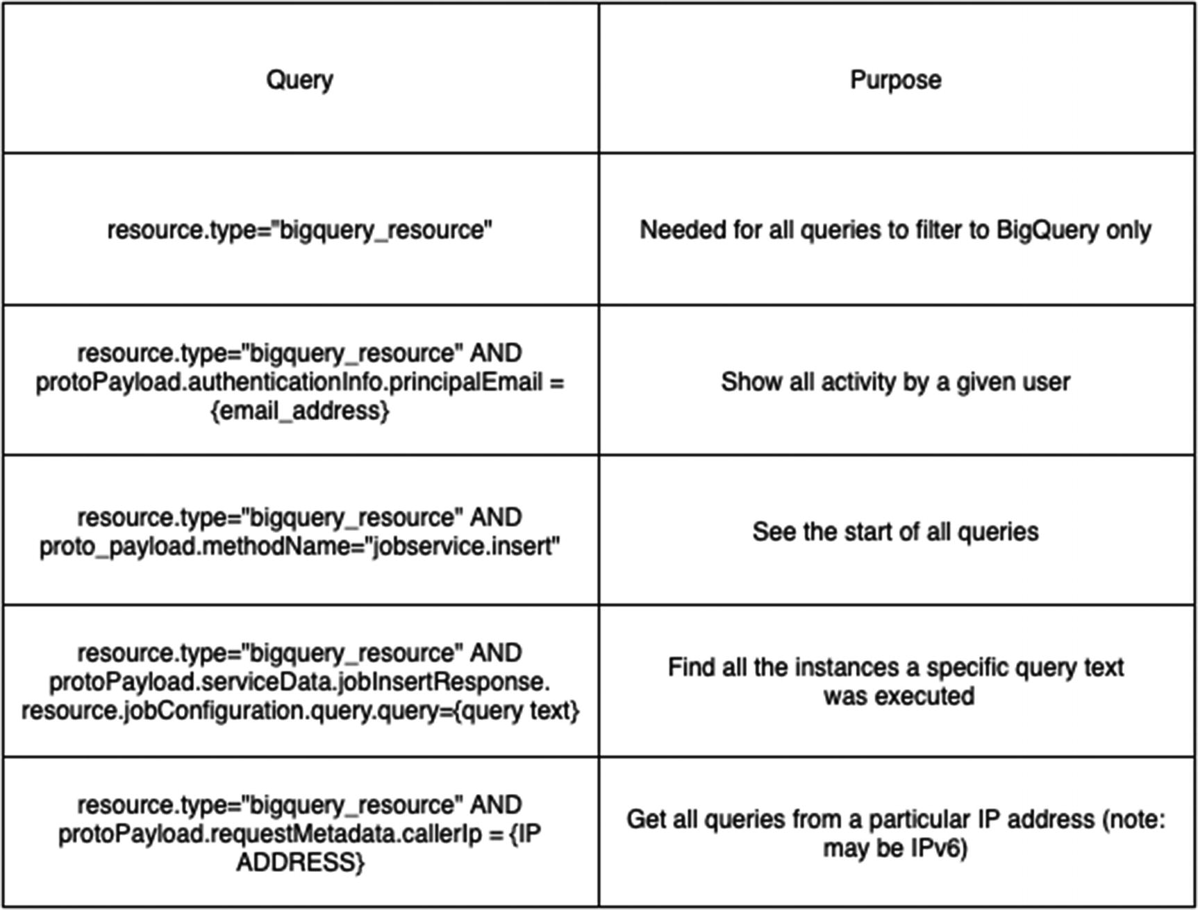
Sample queries for BigQuery logs
If you are looking for several needles in a field of haystacks, this should get you pretty far. If you need to go further back in time or tie together other pieces of data, like the AF Data Crew did, then let’s keep going.
Log Sinks to BigQuery
One of Cloud Logging’s restrictions is that it generally only records up to 30 days’ worth of data2 and only about eight weeks’ worth of metrics. It’s not uncommon to need to analyze logs going back much further for security or compliance reasons or just to track down a pesky application bug that is difficult to replicate.
The restriction makes sense when you consider the nature of the data from both the real-world example and the logging console. For the vast majority of this kind of data, if you don’t need it within a short period of time, you probably won’t ever need it.
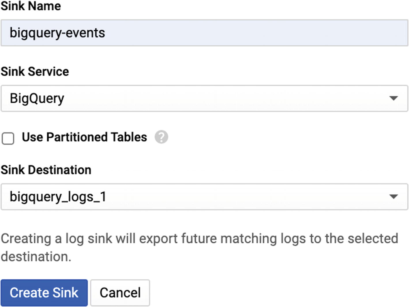
Log sinks to BigQuery
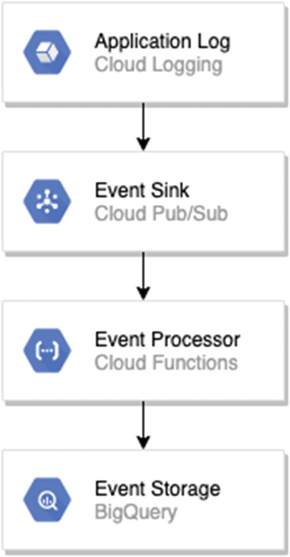
A more complicated pipeline with a log sink
What Is a Sink?
The term “sink” refers to an object that can receive events. As near as I can tell, the etymology of the term is closer to how it is used in electrical engineering, such as the term “heat sink” to indicate a conductor which receives heat from another component and disperses it away. Similarly, a sink is a one-way consumer of one or more other objects producing events. Despite some conceptual commonalities, there’s no relationship to “sync” either. The interaction is purely in a single direction—the producer makes the event and the sink receives it.
Creating a Sink
Making an event sink is very straightforward. It will appear as an option in the “Actions” dropdown on every query result. Click Actions and then “Create Sink” to open the sidebar. Since you can make a sink for any logging query, you can be as broad or narrow as you like. Sizing the query is a bit of an art: you want all the events you might conceivably need for your use cases, but you don’t want to make so many that cost and processing time are too high. If your task requires a sink instead of using Cloud Logging directly, then you can err on the side of including more data. After it has been purged from Cloud Logging, it’s gone forever unless you preserve it in this way.
Name: Obviously you want to assign a descriptive name.
Sink Service: As mentioned previously, the three main options are BigQuery, Cloud Storage, and Pub/Sub. (The fourth option, “Custom Destination”, is actually still the same as the first three, but if you want to log to a different Google cloud project.) Select BigQuery here.
Sink Destination: You have the option to use an existing dataset or make a new one. You can use an existing dataset if you want to create multiple queries that route to the same sink.
After filling this out, click Create. That’s it: all incoming events matching your query will now go to a BigQuery dataset.
An important note: If you do try to log multiple queries to the same sink, remember that the BigQuery schema for a table is set using the first row inserted. If you change anything or the queries have disagreeing schemas, the sink will fail to receive the entries that don’t align. The easiest way to avoid this, of course, is to log each query to a separate table, but you may have a valid reason not to do this. Should you have this problem, it will be sent as an email, appear as a notification on the console activity page for the project, and increment a metric (called exports/error_count).
Additionally, Cloud Logging does a fair amount of field name shortening and alteration to push logs into the BigQuery sink. More importantly, it automatically shards by timestamp using date sharding or partitioning, with date sharding by default. This means that you should use the techniques for querying date-sharded tables when querying the sink.
To edit or delete the sinks, as you would likely want to do with any samples you made, go to the Logs Router on the left sidebar, check the sink(s) you just made, and click Delete. All gone. The dataset being used as the sink will remain intact until you choose to remove it from BigQuery.
To the extent that you are a software engineer or have software engineers in your organization, now might be a good time to do a “look what I can do” presentation to open up some possibilities. Many engineering organizations haven’t yet established consistent logging practices, and you may not be as lucky as the AF Data Crew when you go to get data to investigate your problem. Understanding the interplay between any custom applications you have and your ability to administer your data warehouse is key to deriving value. And, as we’ve already seen, you will be able to help them as well.
If your engineers already have a solution, that’s great too. There are countless logging solutions out there—far too many to name. If your organization runs primarily on Amazon Web Services (AWS) , they probably already use Cloudwatch for a similar purpose. I will mention that Google does have a logging agent that you can install on servers inside AWS. And of course you can always use functions-as-a-service techniques from the previous chapter to create pathways from other cloud providers into BigQuery.
Metrics and Alerting
The other major piece of this puzzle is Cloud Monitoring. Monitoring also used to be under the Stackdriver umbrella but now just goes by Monitoring. While Monitoring is not directly related to BigQuery, it is closely related to what we’ve done with logging thus far and also ties into Google Data Studio, which we’ll discuss at a later point.
Creating Metrics
Name: Again, the name of your metric.
Description: Without all of the metadata to inspect, metrics can be somewhat more obscure than sinks. A description helps you remember what exactly you are trying to track.
Labels: You can use labels to split a metric into multiple time series using the value of a field in the relevant log entry. This is a bit beyond the scope of what we’re trying to do here, but you can learn more at https://cloud.google.com/logging/docs/logs-based-metrics/labels.
Units: If your metric measures a specific unit (megabytes, orders, users, errors, instances, etc.), you can specify it here.
Type: Can be Counter or Distribution. Counter simply records the number of times the qualifying event occurred. Distribution metrics allow you to capture the approximate range of metrics along a statistical distribution. They’re also out of scope here, but if you are interested, they are documented by Google at https://cloud.google.com/logging/docs/logs-based-metrics/distribution-metrics.
After you fill this out, you can click Create Metric, and you will have a new value representing the occurrences of this particular Cloud Logging query. To interact with this metric, you can go to “Logs-Based Metrics” on the left sidebar.
Logs-Based Metrics
When you go to the Logs-Based Metrics view, you will see a host of built-in metrics collected by GCP, as well as your custom metric(s) at the bottom. You can do a couple of things with the metric from this page by clicking the vertical ellipsis menu. Notably, you can view the logs associated with this metric. This means that if you decide in the future that the metric data is insufficient, you can “upgrade” it to an event sink by going to the logs and clicking Actions and “Create Sink” to follow the previous process.
You could also have both the metric and the sink for the same log query, using the metric on dashboards and reports, but having the sink available in BigQuery should you need to do deeper analysis.
A Note About Metrics Export
I’m afraid there is no native way to export metrics to BigQuery. If you’re interested in doing this, you’ll have to venture fairly far afield to build your own solution. Google provides a reference implementation for this use case at https://cloud.google.com/solutions/stackdriver-monitoring-metric-export.
As we get into techniques for real-time dashboarding, the value of this may become clearer. Using a system like this allows you to avoid exporting all of the event data when all you may want is the count or rate of events. This is especially true when you want to look at trends over a much longer period of time. In the example at the beginning of this chapter, the AF Data Crew might have opted to log only the number of errors by type and timestamp. This data would still have allowed them to join in the order data to see that the error rate was higher when the average order price was higher. It would not, however, have allowed them to conclusively determine that the orders experiencing failures were precisely the same orders as the ones with high costs.
There are also countless providers of real-time application monitoring, metrics collection, and so on. Depending on how your organization utilizes the cloud, your solutions for this problem may not involve BigQuery at all.
Alerting
The other tool traditionally associated with the product formerly known as Stackdriver is Alerting. Alerting connects to your metrics and provides a notification system when a metric’s value leaves a desired range. Alerting goes beyond Cloud Logging and can also be used for application health monitoring, performance checks, and so on. Most of these use cases are out of the scope of BigQuery. However, there are a couple of interesting recipes you might build with them.
Business-Level Metrics
Since you can alert on any custom metric, this means you could create alerts for things outside the DevOps scope. In the example at the beginning of this chapter, recall that the issue turned out to be high order cost causing credit cards to exceed their credit limits. Using this knowledge, you could create an alert that fires whenever the failures per dollar exceed a certain ratio. This would be an indication to your business users to check the report or dashboard or to look at the BigQuery order data and see what is causing the anomaly.
Logging Alerts to BigQuery
If you find the alert heuristics useful and want to leverage the automatic aggregation and detection that Cloud Monitoring gives you, you can specify that alerts go to a Cloud Pub/Sub as a notification channel. Then, using techniques in the previous chapter, you can build a Cloud Function that logs the alert to BigQuery and keeps a record of past alerts. (Make sure you don’t create an infinite loop doing this…)
ChatOps
Creating applications leveraging organizational messaging apps is growing increasingly common. Cloud Monitoring supports notification to Slack, email, SMS, and so on natively, but you could also build an application that allows users to acknowledge and dig into the cause for a given alert. For example, an alert might trigger a message to a relevant Slack channel with details about the error condition, but also link to a BigQuery-powered view to look at the data causing it.
Feedback Loops
Way back in Chapter 2, I laid out a rubric for assessing your own organization’s data maturity. The rubric references feedback loops as a key mechanic to achieve a higher degree of maturity. That concept specifically bears revisiting now as we wrap up Part 3. If you have successfully completed your project charter and are looking down the road to the future, you have likely also thought about this in some form. Luckily, you have everything in place to move to the next level. If you’ll permit me the discursion, let’s step up a bunch of levels from organizational theory and look at the dynamics themselves.
The concept of feedback loops arises in innumerable disciplines across history. The first recorded feedback loop was invented in 270 BCE when Ctesibius of Alexandria created a water float valve to maintain water depth at a constant level. The term itself is at least a hundred years old. The feedback loop, at heart, is the recognition that a system’s output is used as part of its input. The system changes itself as it operates. This has profound implications for the understanding of any functioning system. (It’s also, in a lot of ways, the opposite of the sink concept we discussed earlier in the chapter.)
In a way, human history has progressed in tandem with the shortening of feedback loops. Consider the amount of time delivering a message has taken throughout history. Assuming it arrived at all, a transatlantic letter took months to arrive at its destination in the 17th and 18th centuries. By the 19th century, that had shrunk to days. In the early 20th century, the first transatlantic Morse code messages were arriving and dropping times to hours, minutes, and seconds. Now, I can ping a server from the west coast of the United States to the United Kingdom in less than 200 milliseconds and not even think twice about it.
What I am getting at is that the faster a message can be received and interpreted, the faster it can be acted upon and another message sent. While there are many reasons to construct a data warehouse, including business continuity, historical record keeping, and, yes, data analysis, the real additional value in constructing one today is the promise of shortening feedback loops. Not only can you shorten them but you can also dramatically increase the complexity of messages and their effects on the system. Major organizations are adopting one-to-one personalization techniques to address their consumers on an individual basis. Technologies like BigQuery level that playing field so that even smaller organizations can begin implementing these insights without extreme cost or concession.
This won’t happen evenly across your organization or its functions. There’s also no single blueprint to making good interpretations or good decisions based on those interpretations. In fact, without the mediation of data scientists and statisticians, business leaders might jump to the wrong conclusion. This risk increases measurably if there is a risk the data is inaccurate, as it might have been at lower levels of organizational maturity. Using these tools is a foundational part of the strategy, but it is not the only part.
I encourage you to think about ways in which you have already shortened certain feedback loops and can shorten others. More transformationally, you can now begin to think about new feedback loops, like the credit card acceptance scenario we looked at. Adding even more data sources into the mix, as we’ll see in Part 5, can take feedback loops out of the organization and into the world at large. As more organizations, government agencies, and other groups put their datasets into the public domain, you can create feedback loops that understand and react to human behavior itself.
Summary
Cloud Logging, formerly called Stackdriver, is a scaled logging solution attached to all services on the Google Cloud Platform. It receives events automatically from across GCP, as well as custom applications and external sources that you can define. The logging console has a robust searching mechanism to look at events, but they can be persisted for only a maximum of 30 days. Using sinks, you can persist the data indefinitely to BigQuery, where you can analyze and connect it to other data. Cloud Monitoring allows you to synthesize information from logs into real-time dashboards and insights. These tools are both critical in shortening the length of feedback loops and delivering ever-increasing business value.
In the next chapter, we’ll return to the familiar ground of SQL and discuss more advanced concepts you can implement in your data warehouse.