In this chapter, we introduce a propagation source estimator under snapshot observations: a sample path based source estimator (Jordan Center). According to Chap. 5, a snapshot provides partial knowledge of network status at a given time t. Many approaches have been proposed to identify propagation sources under snapshot observations, including Jordan Center, Dynamic Message Passing, effective distance based method, etc. Within these methods, Jordan center is a representative one and many variations and improvements have been made based on this method. Here, we present the details of the Jordan Center estimator. For the techniques involved in other methods under snapshot observations, readers could refer to Chap. 9 for details.
7.1 Introduction
Malicious attack propagation in networks refer to the spread process of attack throughout the networks, and have been widely used to model many real-world phenomena such as the spreading of rumors over online social networks, and the spreading of computer virus over the Internet. The problem of identifying propagation source has attracted many attentions. For example, Shah and Zaman proposed Rumor Center to identify rumor propagation sources [160–162] was analyzed in [160, 161]. They formulated the problem as a maximum likelihood estimation (MLE) problem, and developed novel algorithms to detect the source. However, these methods are considered under the complete observation of networks, which is not applicable for many real-world scenarios. Zhu and Ying [200] considered the following problem: given a snapshot of the diffusion process at time t, can we tell which node is the source of the propagation?
Zhu and Ying [200] adopted the Susceptible-Infected-Recovered (SIR) model, a standard model of epidemics [12, 47]. The network is assumed to be an undirected graph and each node in the network has three possible states: susceptible (S), infected (I), and recovered (R). Nodes in state S can be infected and change to state I, and nodes in state I can recover and change to state R. Recovered nodes cannot be infected again. Initially, all nodes are assumed to be in the susceptible state except one infected node. The infected node is the propagation source of the malicious attack. The source then infects its neighbors, and the attack starts to spread in the network. Now given a snapshot of the network, in which some nodes are infected nodes, some are healthy (susceptible and recovered) nodes. The susceptible nodes and recovered nodes assumed to be indistinguishable. Zhu and Ying [200] proposed a low complexity algorithm, called reverse infection algorithm, through finding the sample path based estimator in the underlying network. In the algorithm, each infected node broadcasts its identity in the network, the node who first collect all identities of infected nodes declares itself as the information source. They proved that the estimated source node is the node with the minimum infection eccentricity. Since a node with the minimum eccentricity in a graph is called the Jordan center, they call the nodes with the minimum infection eccentricity the Jordan infection centers.
7.2 The SIR Model for Information Propagation
Consider an undirected graph G(V, E), where V is the set of nodes and E is the set of undirected edges. Each node v ∈ V has three possible states: susceptible (S), infected (I), and recovered (R). Zhu and Ying [200] assumed a time slotted system. Nodes change their states at the beginning of each time slot, and the state of node v in time t is denoted by X
v(t). Initially, all nodes are in state S except source node v
∗ which is in state I. At the beginning of each time slot, each infected node infects its susceptible neighbors with probability q. Each infected node recovers with probability p. Once a node get recovered, it cannot be infected again. Then, the infection process can be modeled as a discrete time Markov chain X(t), where X(t) = {X
v(t), v ∈ V } is the states of all the nodes at time t. The initial state of this Markov chain is X
v(0) = S for v ≠ v
∗ and  .
.


An example of information propagation
7.3 Maximum Likelihood Detection

![$$\displaystyle \begin{aligned} \hat{v} \in \mbox{arg}~ \displaystyle \max_{v\in V} \displaystyle\sum_{\mathbf{X}[0,t]:\mathbf{F}(\mathbf{X}(t))=\mathbf{Y}} \mbox{Pr}(\mathbf{X}[0, t]|v^* = v), \end{aligned} $$](../images/466717_1_En_7_Chapter/466717_1_En_7_Chapter_TeX_Equ3.png)
Note that the difficulty of solving the problem in (7.3) is the curse of dimensionality. For each v such that Y v = 0, its infection time and recovered time are required, i.e., O(t 2) possible choices; for each v such that Y v = 1, the infection time needs to be considered, i.e., O(t) possible choices. Therefore, even for a fixed t, the number of possible sample paths is at least at the order of t N, where N is the number of nodes in the network. This curse of dimensionality makes it computational expensive. Zhu and Ying [200] introduced a sample path based approach to overcome the difficulty.
7.4 Sample Path Based Detection
![$$\displaystyle \begin{aligned} {\mathbf{X}}^*[0, t^*] = \mbox{arg}~\displaystyle \max_{t,\mathbf{X}[0,t]\in \mathcal{X}(t)}Pr(\mathbf{X}[0,t]), \end{aligned} $$](../images/466717_1_En_7_Chapter/466717_1_En_7_Chapter_TeX_Equ4.png)
![$$\mathcal {X}=\{\mathbf {X}[0,t]|\mathbf {F}(\mathbf {X}(t))=\mathbf {Y}\}$$](../images/466717_1_En_7_Chapter/466717_1_En_7_Chapter_TeX_IEq2.png) . The source node associated with X
∗[0, t
∗] is viewed as the information source.
. The source node associated with X
∗[0, t
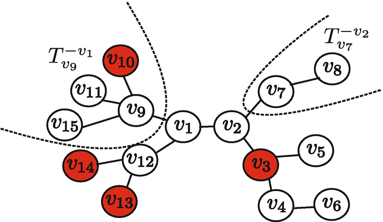
∗] is viewed as the information source. given Y as the maximum distance between v and any infected nodes in the graph. Then, the Jordan infection centers of a graph are the nodes with the minimum infection eccentricity given Y. In Fig. 7.2, nodes v
3, v
10, v
13 and v
14 are observed to be infected. The infection eccentricities of v
1, v
2, v
3, v
4 are 2, 3, 4, 5, respectively, and the Jordan infection center is v
1.
An example illustrating the infection eccentricity
 such that
 ![$$\displaystyle \begin{aligned} t^*_{v_r} = \mbox{arg}~ \displaystyle \max_{t,\mathbf{X}[0,t]} Pr(\mathbf{X}[0,t]|v^* = v_r), \end{aligned} $$](../images/466717_1_En_7_Chapter/466717_1_En_7_Chapter_TeX_Equ5.png)
 is the time duration of the optimal sample path in which v
r is the information source. They proved that
  equals to the infection eccentricity of node v
r. In the second step, they consider two neighboring nodes, say nodes v
1 and v
2. They proved that if
  , then the optimal sample path rooted at v
1 occurs with a higher probability than the optimal sample path rooted at v
2. At the third step, they proved that given any two nodes u and v, if v has the minimum infection eccentricity and u has a larger infection eccentricity, then there exists a path from u to v along which the infection eccentricity monotonically decreases, which implies that the source of the optimal sample path must be a Jordan infection center. For example, in Fig. 7.2, node v
4 has a larger infection eccentricity than v
1 and v
4 → v
3 → v
2 → v
1 is the path along which the infection eccentricity monotonically decreases from 5 to 2. In the next subsection, we briefly explain the techniques involved in these three steps.
, then the optimal sample path rooted at v
1 occurs with a higher probability than the optimal sample path rooted at v
2. At the third step, they proved that given any two nodes u and v, if v has the minimum infection eccentricity and u has a larger infection eccentricity, then there exists a path from u to v along which the infection eccentricity monotonically decreases, which implies that the source of the optimal sample path must be a Jordan infection center. For example, in Fig. 7.2, node v
4 has a larger infection eccentricity than v
1 and v
4 → v
3 → v
2 → v
1 is the path along which the infection eccentricity monotonically decreases from 5 to 2. In the next subsection, we briefly explain the techniques involved in these three steps.7.5 The Sample Path Based Estimator
Lemma 7.1
 , then the following inequality holds
![$$\displaystyle \begin{aligned} \displaystyle \max_{\mathbf{X}[0,t_1]\in \mathcal{X}(t_1)} Pr(\mathbf{X}[0,t_1]) > \max_{\mathbf{X}[0,t_2]\in \mathcal{X}(t_2)} Pr(\mathbf{X}[0,t_2]), \end{aligned} $$](../images/466717_1_En_7_Chapter/466717_1_En_7_Chapter_TeX_Equ6.png)
![$$\mathcal {X}(t)=\{\mathbf {X}[0,t]|\mathbf {F}(\mathbf {X}(t))=\mathbf {Y}\}$$](../images/466717_1_En_7_Chapter/466717_1_En_7_Chapter_TeX_IEq9.png) . In addition,
. In addition,

where d(v r, u) is the length of the shortest path between and u and also called the distance between v r and u, and I is the set of infected nodes.
This lemma states that the optimal time is equal to the infection eccentricity. The next lemma states that the optimal sample path rooted a node with a smaller infection eccentricity is more likely to occur.
Lemma 7.2
 , then
 ![$$\displaystyle \begin{aligned} Pr({\mathbf{X}}^*_u([0, t^*_u])) < Pr({\mathbf{X}}^*_v([0, t^*_v])), \end{aligned} $$](../images/466717_1_En_7_Chapter/466717_1_En_7_Chapter_TeX_Equ8.png)
where
![$${\mathbf {X}}^*_u([0, t^*_u])$$](../images/466717_1_En_7_Chapter/466717_1_En_7_Chapter_TeX_IEq11.png) is the optimal sample path starting from node u.
is the optimal sample path starting from node u.
Proof
Denote by T
v the tree rooted in v and  the tree rooted at u but without the branch from v. See
  and
and  in Fig. 7.2. Furthermore, denote by
  the set of children of v. The sample path X[0, t] restricted to
  is defined to be
 ![$$\mathbf {X}([0,t], T^{-v}_u)$$](../images/466717_1_En_7_Chapter/466717_1_En_7_Chapter_TeX_IEq17.png) .
.
The first step is to show  . Note that
  , otherwise, all infected node are on
  . As T is a tree, v can only reach nodes in
  through edge (u, v),
  , which contradicts
  .
.
 ,
,  , then
 ,
, 


 .
. on the sample path
 ![$${\mathbf {X}}^*_u([0, t^*_u])$$](../images/466717_1_En_7_Chapter/466717_1_En_7_Chapter_TeX_IEq29.png) . If
. If  on
on ![$${\mathbf {X}}^*_u([0, t^*_u])$$](../images/466717_1_En_7_Chapter/466717_1_En_7_Chapter_TeX_IEq31.png) , then
, then 
 and
and  , within
  time slots, node v can infect all infected nodes on
  . Since
  , the infected node farthest from node u must be on
  , which implies that there exists a node
  such that
  and
and  . So node v cannot reach a within
  time slots, which contradicts the fact that the infection can spread from node v to a within
  time slots along the sample path
 ![$${\mathbf {X}}^*_u[0, t^*_u ]$$](../images/466717_1_En_7_Chapter/466717_1_En_7_Chapter_TeX_IEq43.png) . Therefore,
. Therefore,  .
.![$${\mathbf {X}}^*_u([0, t^*_u])$$](../images/466717_1_En_7_Chapter/466717_1_En_7_Chapter_TeX_IEq45.png) , the third step is to construct
, the third step is to construct ![$${\mathbf {X}}^*_v([0, t^*_v])$$](../images/466717_1_En_7_Chapter/466717_1_En_7_Chapter_TeX_IEq46.png) which occurs with a higher probability. The sample path
which occurs with a higher probability. The sample path ![$${\mathbf {X}}^*_u([0, t^*_u])$$](../images/466717_1_En_7_Chapter/466717_1_En_7_Chapter_TeX_IEq47.png) can be divided into two parts along subtrees
can be divided into two parts along subtrees  and
and  . Since
  , then
 ![$$\displaystyle \begin{aligned} Pr({\mathbf{X}}^*_u([0, t^*_u])) = q\cdot Pr({\mathbf{X}}^*_u([0, t^*_u], T^{-u}_v)|t^I_v=1) \cdot Pr({\mathbf{X}}^*_u([0, t^*_u], T^{-v}_u)). \end{aligned} $$](../images/466717_1_En_7_Chapter/466717_1_En_7_Chapter_TeX_Equ14.png)
![$${\mathbf {X}}^*_v([0, t^*_v])$$](../images/466717_1_En_7_Chapter/466717_1_En_7_Chapter_TeX_IEq51.png) , node u was infected at the first time slot, then
, node u was infected at the first time slot, then ![$$\displaystyle \begin{aligned} Pr({\mathbf{X}}^*_v([0, t^*_v])) = q\cdot Pr({\mathbf{X}}^*_v([0, t^*_v], T^{-u}_v)|t^I_v=1) \cdot Pr({\mathbf{X}}^*_v([0, t^*_v], T^{-v}_u)|t^I_u=1). \end{aligned} $$](../images/466717_1_En_7_Chapter/466717_1_En_7_Chapter_TeX_Equ15.png)
 , given
 ![$${\mathbf {X}}^*_u([0, t^*_u], T^{-u}_v)$$](../images/466717_1_En_7_Chapter/466717_1_En_7_Chapter_TeX_IEq53.png) , in which
, in which  , the partial sample path
 ![$${\mathbf {X}}^*_v([0, t^*_v], T^{-u}_v)$$](../images/466717_1_En_7_Chapter/466717_1_En_7_Chapter_TeX_IEq55.png) can be constructed to be identical to
can be constructed to be identical to ![$${\mathbf {X}}^*_u([0, t^*_u], T^{-u}_v)$$](../images/466717_1_En_7_Chapter/466717_1_En_7_Chapter_TeX_IEq56.png) except that all events occur one time slot earlier, i.e.,
except that all events occur one time slot earlier, i.e., ![$$\displaystyle \begin{aligned} {\mathbf{X}}^*_v([0, t^*_v], T^{-u}_v) = {\mathbf{X}}^*_u([0, t^*_u], T^{-u}_v). \end{aligned} $$](../images/466717_1_En_7_Chapter/466717_1_En_7_Chapter_TeX_Equ16.png)
![$$\displaystyle \begin{aligned} Pr({\mathbf{X}}^*_u([0, t^*_u], T^{-u}_v)|t^Iv=1) = Pr({\mathbf{X}}^*_v([0, t^*_v], T^{-u}_v)).. \end{aligned} $$](../images/466717_1_En_7_Chapter/466717_1_En_7_Chapter_TeX_Equ17.png)
 ,
, ![$${\mathbf {X}}^*_v([0, t^*_v], T^{-v}_u)$$](../images/466717_1_En_7_Chapter/466717_1_En_7_Chapter_TeX_IEq58.png) can be constructed such that
can be constructed such that ![$$\displaystyle \begin{aligned} {\mathbf{X}}^*_v([0, t^*_v], T^{-v}_u)\in \mbox{arg}~\displaystyle \max_{\tilde{\mathbf{X}}([0,t^*_v], t^{-v}_u)\in\mathcal{X}(t^*_v, T^{-v}_u)}Pr(\tilde{\mathbf{X}}([0,t^*_v], t^{-v}_u)|t^I_u=1). \end{aligned} $$](../images/466717_1_En_7_Chapter/466717_1_En_7_Chapter_TeX_Equ18.png)
![$$\displaystyle \begin{aligned} \begin{array}{lll} \displaystyle \max_{\tilde{\mathbf{X}}([0,t^*_v], t^{-v}_u)\in\mathcal{X}(t^*_v, T^{-v}_u)}Pr(\tilde{\mathbf{X}}([0,t^*_v], t^{-v}_u)|t^I_u=1)\\ =\displaystyle \max_{\tilde{\mathbf{X}}([0,t^*_u-1], t^{-v}_u)\in\mathcal{X}(t^*_u-1, T^{-v}_u)}Pr(\tilde{\mathbf{X}}([0,t^*_u-1], t^{-v}_u)|t^I_u=1)\\ >\displaystyle \max_{\tilde{\mathbf{X}}([0,t^*_u], t^{-v}_u)\in\mathcal{X}(t^*_u, T^{-v}_u)}Pr(\tilde{\mathbf{X}}([0,t^*_u], t^{-v}_u))\\ \end{array} \end{aligned} $$](../images/466717_1_En_7_Chapter/466717_1_En_7_Chapter_TeX_Equ19.png)
The following lemma gives a useful property of the Jordan infection centers.
Lemma 7.3
On a tree network with at least one infected node, there exist at most two Jordan infection centers. When the network has two Jordan infection centers, the two must be neighbors.
The following theorem states that the sample path based estimator is one of the Jordan infection centers.
Theorem 7.1

Proof
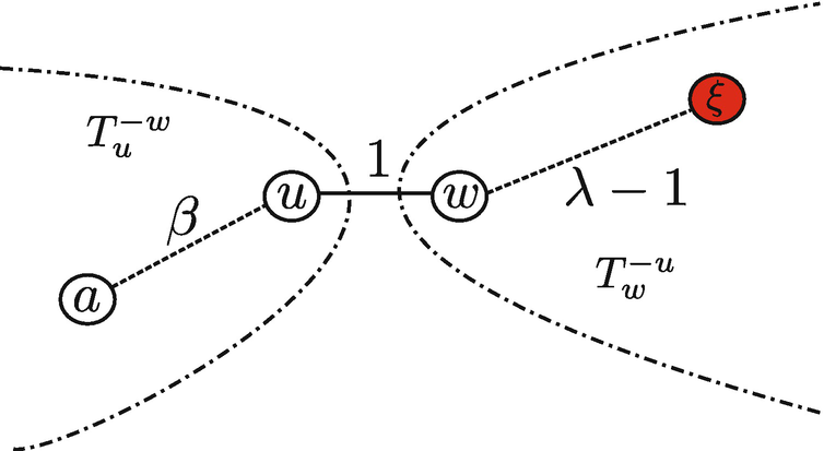
Assume the network has two Jordan infection centers: w and u, and assume  . Based on Lemma 7.3, w and u must be adjacent. The following steps show that, for any a ∈ V ∖{w, u}, there exists a path from a to u (or w) along which the infection eccentricity strictly decreases.
 . Then, there exists a node ξ such that the equality holds. Suppose that d(γ, w) ≤ λ − 2 for any
  , which implies
 ,
, 

 . Therefore, there exists
  such that

A pictorial description of the positions of nodes a, u, w and ξ


 and d(a, u) = β, then for any
  , we have
 such that the equality holds. On the other hand,


Repeatedly applying Lemma 7.2 along the path from node a to u, then the optimal sample path rooted at node u is more likely to occur than the optimal sample path rooted at node a. Therefore, the root node associated with the optimal sample path X ∗[0, t ∗] must be a Jordan infection center. The theorem holds.
7.6 Reverse Infection Algorithm
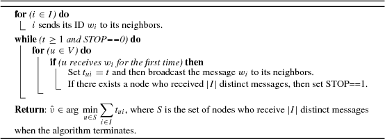
Zhu and Ying [200] further proposed a reverse infection algorithm to identify the Jordan infection centers. The key idea of the algorithm is to let every infected node broadcast a message containing its identity (ID) to its neighbors. Each node, after receiving messages from its neighbors, checks whether the ID in the message has been received. If not, the node records the ID (say v), the time at which the message is received (say t
v), and then broadcasts the ID to its neighbors. When a node receives the IDs of all infected nodes, it claims itself as the propagation source and the algorithm terminates. If there are multiple nodes receiving all IDs at the same time, the tie is broken by selecting the node with the smallest  . The details of the algorithm is presented in Algorithm 7.1.
Simulations on g-regular trees were conducted. The infection probability q was chosen uniformly from (0, 1) and the recovery probability p was chosen uniformly from (0, q). The infection process propagates t was uniformly chosen from [3, 20]. The experimental results show that the detection rates of both the reverse infection and closeness centrality algorithms increase as the degree increases and is higher than 60% when g > 6.
Algorithm 7.1: Reverse infection algorithm
