In this chapter, we introduce a propagation source estimator under sensor observations: Gaussian source estimator. According to Chap. 5, sensors are firstly injected into networks, and then the propagation dynamics over these sensor nodes are collected, including their states, state transition time and infection directions. There have been many approaches proposed under sensor observations, including Bayesian based method, Gaussian based method, Moon-Walk based method, etc. Here, we particular present the details of the Bayesian based method. For the techniques involved in other methods, readers could refer to Chap. 9 for details.
8.1 Introduction
Localizing the source of a malicious attack, such as rumors or computer viruses, is an extremely desirable but challenging task. The ability to estimate the source is invaluable in helping authorities contain the malicious attacks or infection. In this context, the inference of the unknown source was analyzed in [160, 161]. These methods assume that we know the state of all nodes in the network. However, having the observation on an entire network is hardly possible. Pinto et al. [146] proposed to locate the source of propagation under the practical constraint that only a small fraction of nodes can be observed. This is the case, for example, when locating a spammer who is sending undesired emails over the internet, where it is clearly impossible to monitor all the nodes. Thus, the main difficulty is to develop tractable estimators that can be efficiently implemented (i.e., with subexponential complexity), and that perform well on multiple topologies.
8.2 Network Model
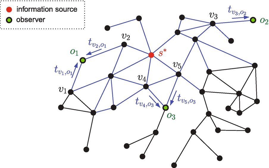
Source estimation on graph G. At time t = t ∗, the propagation source s ∗ initiates the propagation of a malicious attack. In this example, there are three observers/sensors, which measure from which neighbors and at what time they were attacked. The goal is to estimate, from these observations, which node in G is the propagation source
The propagation process is modeled as follows. At time t, each vertex u ∈ G presents one of two possible statuses: (a) infected, if it has already been attacked from any of its neighbors; or (b) susceptible, if it has not been infected/attacked so far. Let V (u) denote the set of vertices directly connected to u, i.e., the neighborhood or vicinity of u. Suppose u is in the susceptible state and, at time t u, receives the attack for the first time from one neighbor, say s, thus becoming infected. Then, u will re-transmit the malicious attack to all its other neighbors, so that each neighbor v ∈ V (u)∖s receives the attack at time t u + θ uv, where θ uv denotes the random propagation delay associated with edge (u, v). The random variables {θ uv} for different edges (u, v) have a known, arbitrary joint distribution. The propagation process is initiated by the source x ∗ at an unknown time t = t ∗.
Let  denote the set of K observers/sensors, whose location on the network G is already known. Each observer measures from which neighbor and at what time it received the attack. Specifically, if t
v,o denotes the absolute time at which observer o receives the attack from its neighbor v, then the observation set is composed of tuples of direction and time measurements, i.e.,
denote the set of K observers/sensors, whose location on the network G is already known. Each observer measures from which neighbor and at what time it received the attack. Specifically, if t
v,o denotes the absolute time at which observer o receives the attack from its neighbor v, then the observation set is composed of tuples of direction and time measurements, i.e.,  , for all o ∈ O and v ∈ V (o).
8.3 Source Estimator
 such that the localization probability
  is maximized. Since s
∗ is assumed to be uniformly random over the network G, the optimal estimator is the maximum likelihood (ML) estimator,
is maximized. Since s
∗ is assumed to be uniformly random over the network G, the optimal estimator is the maximum likelihood (ML) estimator, 
 between the source s and the observers in the graph G. The set
  represents the propagation delays for all edges of the graph G. The deterministic function g depends on the joint distribution of the propagation delays. Note that, the estimator in Eq. (8.1) is calculated through averaging over two different sources of randomness: (a) the uncertainty in the paths that the attack takes to reach the observers, and (b) the uncertainty in the time that the attack takes to cross the edges of the graph G. Due the combinatorial nature of Eq. (8.1), its complexity increases exponentially with the number of nodes in G, and is therefore intractable. In order to address this problem, Pinto et al. [146] proposed a method of complexity O(N) that is optimal for general trees, and a strategy of complexity O(N
3) that is suboptimal for general graphs.
represents the propagation delays for all edges of the graph G. The deterministic function g depends on the joint distribution of the propagation delays. Note that, the estimator in Eq. (8.1) is calculated through averaging over two different sources of randomness: (a) the uncertainty in the paths that the attack takes to reach the observers, and (b) the uncertainty in the time that the attack takes to cross the edges of the graph G. Due the combinatorial nature of Eq. (8.1), its complexity increases exponentially with the number of nodes in G, and is therefore intractable. In order to address this problem, Pinto et al. [146] proposed a method of complexity O(N) that is optimal for general trees, and a strategy of complexity O(N
3) that is suboptimal for general graphs.8.4 Source Estimator on a Tree Graph
 is called the set of K
a active observers. The observations made by the nodes in O
a provide two types of information. (a) The first information is the direction in which attack arrives to the active observers, which uniquely determines a subset T
a ∈ T of regular nodes. Hence, T
a is called active subtree, (see the left figure in Fig. 8.2). (b) The second information is the timing at which the attack arrives to the active observers, denoted by
is called the set of K
a active observers. The observations made by the nodes in O
a provide two types of information. (a) The first information is the direction in which attack arrives to the active observers, which uniquely determines a subset T
a ∈ T of regular nodes. Hence, T
a is called active subtree, (see the left figure in Fig. 8.2). (b) The second information is the timing at which the attack arrives to the active observers, denoted by  , which is used to localize the source within the set T
a. It is also convenient to label the edges of T
a as E(T
a) = {1, 2, ⋯ , E
a}, so that the propagation delay associated with edge i ∈ E is denoted by θ
i (see the left figure in Fig. 8.2). Assume that the propagation delays associated with the edges of T are independent identically distributed random variables with Gaussian distribution N(μ, σ
2), where the mean μ and variance σ
2 are known. Based on these definitions, the following result can be concluded.
, which is used to localize the source within the set T
a. It is also convenient to label the edges of T
a as E(T
a) = {1, 2, ⋯ , E
a}, so that the propagation delay associated with edge i ∈ E is denoted by θ
i (see the left figure in Fig. 8.2). Assume that the propagation delays associated with the edges of T are independent identically distributed random variables with Gaussian distribution N(μ, σ
2), where the mean μ and variance σ
2 are known. Based on these definitions, the following result can be concluded.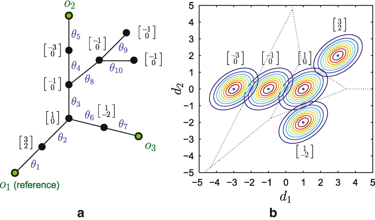
(a) Active tree T
a. The vector next to each candidate source s is the normalized deterministic delay  . The normalized delay covariance for this tree is
 ![$$\tilde {\mathbf {A}}:=\mathbf {A}/\sigma ^2=[5,2;2,4]$$](../images/466717_1_En_8_Chapter/466717_1_En_8_Chapter_TeX_IEq10.png) . (b) Equiprobability contours of the probability density function P(d|s
∗ = s) for all s ∈ T
a, and the corresponding decision regions. For a given observation d, the optimal estimator chooses the source s that maximizes P(d|s
∗ = s)
. (b) Equiprobability contours of the probability density function P(d|s
∗ = s) for all s ∈ T
a, and the corresponding decision regions. For a given observation d, the optimal estimator chooses the source s that maximizes P(d|s
∗ = s)
Proposition 8.1 (Optimal Estimation in General Trees)

![$$\displaystyle \begin{aligned}{}[\mathbf{d}]_k = t_{k+1} - t_k, \end{aligned} $$](../images/466717_1_En_8_Chapter/466717_1_En_8_Chapter_TeX_Equ3.png)
![$$\displaystyle \begin{aligned}{}[\boldsymbol{\mu}_s]_k = \mu(|P(s,o_{k+1})| - |P(s,o_1)|), \end{aligned} $$](../images/466717_1_En_8_Chapter/466717_1_En_8_Chapter_TeX_Equ4.png)
![$$\displaystyle \begin{aligned}{}[\mathbf{A}]_{k,i} = \sigma^2\times \left\{ \begin{array}{ll} |P(o_1,o_{k+1})|, & k=i,\\ |P(o_1,o_{k+1}) \cap P(1,o_{i+1})|, & k\neq i,\\ \end{array} \right. \end{aligned} $$](../images/466717_1_En_8_Chapter/466717_1_En_8_Chapter_TeX_Equ5.png)
for k, i = 1, ⋯ , K a − 1, with |P(u, v)| denoting the number of edges (i.e., the length) of the path connecting vertices u and v. Readers could refer to [ 146 ] for the detailed proof of this proposition.
Note that, when node s is chosen as the source, μ s and A represent, respectively, the mean and covariance of the observed delay d (see Fig. 8.1 for illustration).

8.5 Source Estimator on a General Graph

 , with parameters μ
s and A
s computed with respect to the BFS tree T
bfs,s rooted at s. It can easily shown that the complexity of Eq. (8.7) scales subexponentially with N, as O(N
3).
, with parameters μ
s and A
s computed with respect to the BFS tree T
bfs,s rooted at s. It can easily shown that the complexity of Eq. (8.7) scales subexponentially with N, as O(N
3).Therefore, Eqs. (8.2) and (8.7) gives the propagation source estimator for a tree graph and a general graph, respectively. The computational complexity of these two estimators are O(N) and O(N 3), respectively. We call these estimators as Gaussian source estimators.
To test the effectiveness of the proposed approach, Pinto et al. [146] used the well-documented case of cholera outbreak that occurred in the KwaZulu-Natal province, South Africa, in 2000. Propagation source identification was performed by monitoring the daily cholera cases reported in K communities (the observers). The experimental results show that by monitoring only 20% of the communities, the Gaussian estimator achieves an average error of less than four hops between the estimated source and the first infected community. This small distance error may enable a faster emergency response from the authorities in order to contain an outbreak.