3

Comparison and Causality

[Economics] undertakes to study the effects which will be produced by certain causes, not absolutely, but subject to the condition that other things are equal, and the causes are able to work out their effects undisturbed. Almost every scientific doctrine … will be found to contain some proviso to the effect that other things are equal: the action of the causes in question is supposed to be isolated; certain effects are attributed to them, but only on the hypothesis that no cause is permitted to enter except those distinctly allowed for.

—Alfred Marshall²⁶²

The prior chapter showed that one never fully measures fitness. The first section of this chapter argues that comparative predictions provide a way forward. A comparative prediction describes how a change in some condition alters a trait, mediated by a fundamental force of design. The logic of comparative predictions and the broad listing of predictions for microbial traits set the primary themes of this book.

The second section contrasts evolutionary and organismal responses. A changed condition may favor an evolutionary response in the population. A change may also trigger a phenotypically plastic organismal response in individuals. In simple cases, theory makes the same comparative prediction for evolutionary response and organismal response.

The third section develops the notion of a fundamental force as a partial cause. To give a physical example, gravity is a fundamental force that acts as a partial cause of motion but is rarely by itself a complete explanation of motion. Comparative predictions isolate fundamental forces and partial causes.

The fourth section briefly reviews recent progress in causal inference. I set the causal study of organismal design within the larger context of formulating and testing causal hypotheses.

The fifth section specifies the structure of comparative predictions. That section also presents notation for writing comparative predictions.

The sixth section reviews the goals and approach. Subsequent chapters develop comparative predictions. Those predictions reveal the fundamental forces that shape microbial design.

3.1 Comparative Predictions

Testable hypotheses follow from comparative predictions. For example, as the genetic correlation and kin selection relatedness between individuals rise within groups, theory predicts greater cooperative and less competitive trait expression. Tests on microbes support that comparative prediction.441 Here, I focus on the structure of comparative predictions and the analysis of causality.

ADVANTAGE OF COMPARISON

Microbes often secrete publicly shared factors, such as iron-scavenging siderophores.^216,235 Once released from a cell, the publicly available molecules can be used by neighboring cells. Greater production by an individual cell cooperatively benefits the local group. By contrast, “cheating” nonproducers outcompete neighbors by using the secreted factors of others and saving the cost of production.

Numerous studies support the comparative kin selection prediction in the introductory paragraph of this section. Under high relatedness, relatively more individuals cooperatively produce a shared public good. Under low relatedness, relatively fewer individuals produce the public good, acting as nonproducing cheaters that outcompete neighbors.²¹⁶

In such comparisons, one does not have to measure all components of fitness. The prediction only requires that, aggregated over a variety of common conditions, there be an overall tendency for increased relatedness to associate with increased cooperative trait expression.

NOTION OF CAUSALITY

Comparison provides a reasonable notion of causality. If I repeatedly observe or make a change in condition A, and the predicted direction of change in B tends to happen under a variety of circumstances, then A seems to be a cause of B. We do not have to know all of the factors involved and all of the different conditions. We only need to know that we predicted a particular direction of change, and we tended to see that direction of change.

Of course, confounding correlations and other difficulties can complicate causal inference. Later sections discuss ways to increase the accuracy of causal analysis.

INFERENCE

Statistical inference for comparisons is often simple.¹⁰⁷ If I predict the direction of change in five independent tests, then the probability that I would be right by chance in all five cases is p = 1/2⁵ ≈ 0.03.

The probability that I would be right by chance 59 or more times in 100 trials is also p ≈ 0.03, from the binomial probability distribution. A prediction with a small tendency in the right direction can provide a significant indication of an underlying force.

We can restate the issue for comparison and public goods. It is difficult to say, in any particular example, whether a certain level of relatedness should be associated with a particular level of public goods secretion. By contrast, we can make a strong prediction about the direction of change in public goods secretion with a change in relatedness.

A comparative directional prediction greatly simplifies inference. We do not need to measure fitness accurately with respect to the broad context that shaped design, a measurement that is usually not possible.

It may not be easy to observe or experimentally create the proper comparison. But without such comparison, there can be no reasonable and broadly applicable way to study the forces of design.

TRADEOFFS

The role of comparison arises in a slightly different way for tradeoffs. For example, it is difficult to say whether a rise in dispersal trades off against a decline in survival. Or whether a pathogen’s benefit from increased transmission between hosts trades off against its cost for greater virulent damage to its host. Such associations between traits depend on the underlying mechanism and various confounding factors.¹⁴³

Consider anthrax as an example of the coupling between virulence and transmission. In some habitats, the dominant mode of anthrax transmission is via airborne spores. After pulmonary infection, the pathogen causes few symptoms during the early stages of spread within the host. Only when the bacteria rise to very high density within the host does anthrax express its severe toxins. Those toxins rapidly kill the host. A dead mammalian carcass dries up and releases vast numbers of spores. The severe virulence relates directly to the mode of transmission.

This analysis of anthrax in terms of a virulence-transmission tradeoff does not arise from a testable hypothesis confronted with meaningful data. Instead, it describes observations for one example. Inference is always weak in the analysis of a single case.

To study whether a particular tradeoff dominates design, we must express a comparative prediction.¹⁴³ For example, as conditions change to increase a hypothesized mechanistic coupling between virulence and transmission, the observed association between those components of fitness should increase.

The challenge here is to find the correct understanding of the biological mechanisms so that one can accurately predict the coupling between fitness components. For example, we might argue that airborne transmission imposes a stronger virulence-transmission tradeoff than does vector-borne transmission. The data may prove us to be either right or wrong about that comparative prediction.

A similar problem concerns the tradeoff between survival and dispersal. Various microbial mechanisms facilitate dispersal, such as the secretion of molecules that aid movement over surfaces. In some situations, the cost of expressing dispersal-related traits may reduce survival. Comparatively, the more patchy resources are over time and space, the more strongly microbes may be favored to trade local survival for dispersal to new patches.

The tradeoff between survival and dispersal also depends on the cost associated with the particular mechanism of dispersal. For a low-cost mechanism, the association between survival and dispersal may be weak because the marginal loss in survival for an increase in dispersal is small. Thus, wide variation in dispersal rate may be only weakly associated with variation in survival and in overall fitness.

The low association between dispersal and fitness would lead to a weak signal in comparative hypotheses. By contrast, strongly associated marginal changes in dispersal costs and fitness benefits would lead to a strong signal in comparative hypotheses.

In summary, we should consider tradeoffs as traits to be studied directly. As for any trait, we make a comparative prediction. Does an altered circumstance predict an increase or decrease in the strength of the tradeoff and its importance in shaping design? Comparative predictions about the direction of change provide the only simple, consistent approach to theory and empirical tests (Fig. 3.1).

Figure 3.1   Each pairwise tradeoff embeds within a multidimensional tradeoff, confounding the direct study of pairwise tradeoffs.300 This plot shows tradeoffs between three traits. Suppose, for example, that x is growth rate, y is biomass yield per unit of food intake, and z is toxin production to kill competitors. Assume fitness is x + by + cz, with the constraint that x² + y² + z² = 1. For fixed values of z, the optimal (x, y) pairs lie along the surface curves perpendicular to the arrow line, often called the Pareto frontier. Comparatively, greater b values predict an increase in y and a decrease in x because of an x versus y tradeoff. The additional z dimension leads to the additional comparative prediction that, as c increases, the optimal (x, y) pairs follow along the surface curve on the unit sphere in which both x and y decrease, as shown in the curve with arrows for b = 2. Thus, we may see rate and yield both decrease as toxin production is increasingly favored. If we did not know about toxin production, it would seem as if observed variation were moving orthogonally to the rate versus yield tradeoff, apparently contradicting the existence of that tradeoff. As long as we focus on explicit comparative predictions in terms of changes in b or changes in c, we have a reasonable chance of matching predictions to the forces that shape design.

The essential role of comparison in the study of biological design is not a new idea.¹⁷³ Darwin emphasized comparison throughout his work. His focus on comparison was one of his great conceptual innovations. Comparison allowed him to revolutionize the analysis and interpretation of historical processes as forces that shape the observed diversity of biological design.

3.2 Evolutionary Response versus Organismal Response

Comparison focuses on change in trait expression. For example, a microbe may increase siderophore secretion in response to an increase in its genetic relatedness with its neighbors.

Traits change in two different ways. First, increased siderophore secretion may be an evolutionary response to changed conditions. The altered conditions favor genetic change in the population, causing an increase in secretion.

Second, increased secretion may be a phenotypically plastic response of individuals to changed conditions. Individuals sense altered conditions and change their trait expression in response. The response function maps each condition to an expression pattern. Evolutionary forces shape the response function.82,321,443

In some simple comparative predictions, we may be able to ignore the distinction between the evolutionary change in trait values and the evolutionary change in trait response functions.

For example, increased relatedness between neighbors will tend to favor greater public goods secretions in both cases. In the first case of fixed trait expression, evolutionary forces will tend to favor genetic change in the population that increases trait expression.

In the second case of phenotypically plastic trait expression, evolutionary forces will tend to favor genetic change in the response function. The favored response function will typically map low relatedness to relatively low expression of public goods secretion and high relatedness to relatively high expression.

In both cases, a change from low to high relatedness predicts increased expression. Evolutionary forces ultimately shape trait expression in the same way. We arrive at the same comparative prediction.

In this simplest description of evolutionary forces and comparative predictions, we do not have to distinguish between evolutionary response and phenotypically plastic organismal response.

The most general approach considers all traits as arising from response functions. Genetically fixed traits sit at one endpoint, such that, for a given genotype, all environments map to the same trait expression. Maximally plastic traits sit at the other endpoint, in which each environment maps to a different expression for the trait.

Must we pay attention to the lability of the response function when formulating comparative hypotheses? The ideal answer is: the more we can do so, the better. The pragmatic answer remains an open problem.

I will often ignore the distinction and focus on comparative predictions for trait values. In some cases, such as explicit consideration of design in the control of plastic trait expression, the response function becomes the focus of analysis.

Future work will need to clarify the limits on simplification. In my view, it is better to start too simply and then add necessary complexity, rather than to start with too much complexity and then subtract to find minimal sufficiency. It is easier to see what is missing in simplicity than it is to see what is not needed in complexity.

3.3 Fundamental Forces and Partial Causes

In physics, gravity is a fundamental force that acts as a partial cause of motion. Gravity by itself rarely provides a complete explanation of motion. In this case, a fundamental force is a component of the various causes of motion.

In biology, I use fundamental force to mean a widespread evolutionary process that shapes organismal design. Only the component forces of natural selection can give rise to design. Other evolutionary forces act as constraints with respect to design.

For example, ephemeral resource patches favor dispersal. Stable resource patches favor local survival. These examples illustrate how resource patch demography influences the relative reproductive value of dispersal and survival. Put another way, resource patch demography is a partial cause of design, mediated by the fundamental force of reproductive value.

When considering the design differences between two microbes, several fundamental forces likely play a role. For example, increased genetic correlation between neighbors alters the fundamental force of kin selection that shapes cooperative traits. A cooperative trait might be secretion of exoenzymes for external digestion or secretion of other shareable public goods.

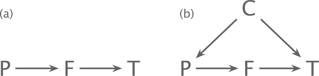
Figure 3.2   Partial causes and causal inference. (a) A partial cause in isolation. The parameter, P, influences the trait, T, mediated by the force, F. (b) A covariate, C, causes an association between the parameter and the trait independently of the mediating force. If the confounding effect of C is not resolved, one may obtain an incorrect estimate for the causal effect of P on T.

Increased genetic correlation may influence two opposing forces. On the one hand, increased correlation enhances the shared genetic interests of neighbors, favoring greater expression of cooperative traits. On the other hand, increased correlation raises the competition between related genotypes, favoring lesser expression of cooperative traits.6,112,333,404,449

In this case, each force acts in a pathway of partial causation. The first partial cause favors higher trait expression. The second partial cause favors lower trait expression. The net effect may be one way or the other, or no change at all. I develop examples of opposing partial causes in subsequent chapters.

Decomposition of change into partial causes provides significant insight into the forces that shape design, perhaps the best insight that we may achieve.

3.4 Causal Inference

Figure 3.2a shows a pathway of partial causation. The parameter, P, influences the microbial trait, T, mediated by the force, F. Partial causation expresses a comparative prediction. A rise in P predicts the direction of change in T. The predicted direction of change depends on how the pathway of partial causation functions.

Partial causation is always embedded within a larger set of causes. In Fig. 3.2b, the covariate, C, influences both the parameter and the trait. Some of the observed association between the parameter and the trait arises from the common cause, C, rather than the focal pathway, P → F → T. Thus, it is often misleading simply to measure how observed variation in a parameter associates with observed changes in a trait.

Figure 3.3   An intervening variable, C, is often mistaken for a covariate, leading to incorrect inference about causality. In Elwert & Winship’s example, given in Pearl & Mackenzie,312 we equate the potentially confounding paths, P → C ← T, with three features of movie actors, Beauty → Celebrity ← Talent. Beauty and talent contribute to celebrity. However, beauty and talent are not associated with each other in the general population. Thus, it would be a mistake to treat C as a covariate when analyzing the relation between P and T, because C does not cause an association between P and T.

To isolate the parameter P’s partial causative effect on the trait, T, we must remove the causal arrows leading into P, or adjust for those causes. Four approaches isolate the causal effect.³¹²

First, controlled randomization of the “treatment” values of P clears potential associations of P with T via indirect confounding causes. In other words, randomization breaks the pathways with arrows going into P. However, it may not be possible to conduct a suitable randomized controlled experiment for the evolutionary response of a trait to changed parameters and evolutionary forces.

Second, one can estimate the causal effect of the parameter separately for each level of each covariate. Conditioning on covariate values removes their potential confounding effect. However, one must successfully identify all of the covariates and then measure them.

The analysis of covariation also requires that one distinguish between a covariate as a common cause, P ← C → T, as in Fig. 3.2b, and an intervening variable that is caused by both the input and the response, P → C ← T, as in Fig. 3.3.

In Fig. 3.3, the variable C does not create an association between P and T. Correcting for C induces a spurious correlation between those variables,³¹² as explained in the caption of Fig. 3.3.

Mistaken correction for an intervening variable happens when the direction of causation is ignored. Direction of causality is rarely considered in standard analyses of covariation, leading to many mistaken inferences.³¹²

In the third approach to isolating the partial causative effect of P, one directly manipulates the value of P, breaking any incoming causal arrows. The change has to be maintained for a sufficiently long period to achieve a full response. In addition, the intervention becomes a new causal influence into P and so must not itself be correlated with T via a confounding pathway.

The fourth approach, counterfactual analysis, estimates how an imagined manipulation of P would change T. In this case, the observed data without manipulations of P can sometimes provide information about how such a change in P would be expected to alter T. The analysis is counterfactual because it runs counter to the factual value of P. Counterfactual analysis has greatly advanced in recent years.^283,312

Those four approaches describe the methods emphasized by Pearl & Mackenzie.³¹² However, in the study of natural history and biological design, one sometimes has to use a weaker observational approach.

If one can aggregate several observed cases of variable P, then any causal paths into P may be sufficiently randomized to reveal the partial causal effect of P on T. Correcting for known correlates, such as common ancestry, strengthens causal insight.

These details support the claim that one can study partial causation in the context of a larger set of causes. The pathways of partial causation are the building blocks of causal understanding.

This book develops hypotheses of partial causation for microbial design. How, in theory, do fundamental forces shape microbial traits? How do environmental and biotic parameters influence those fundamental forces? The broad set of comparative predictions builds the necessary foundation for future progress.

3.5 Structure and Notation of Comparative Predictions

Comparative predictions have the form

Δ parameter ⇒ Δ force ⇒ Δ trait.   (3.1)

A change in a parameter changes a fundamental force, which changes a trait.

A comparative prediction emphasizes how the direction of change in a parameter predicts the direction of change in a trait. A force mediates the causal pathway of change. For example,

P → F ⊣ T

states that an increase in the parameter P causes an increase (→) in the mediating force F, and an increase in F causes a decrease (⊣) in the trait T. The positive and negative effects multiply through a pathway, so the combination of positive (→) and negative (⊣) effects yields a net negative cause P⊣T.

Two negative effects, P ⊣ F ⊣ T, yield a net positive cause, P → T. When a causal effect may be up or down depending on the context, we write P − ↕T.

The example

patch lifespan → mutant overgrowth ⊣ secretion

states that the longer resource patches last (Δ parameter), the greater the selective pressure favoring novel mutants that can overgrow the local population ( Δ force). Overgrowth mutants may gain their advantage by not secreting external, shareable factors, such as exoenzymes used to digest complex carbohydrates (Δ trait). Reduced secretion of publicly shared factors saves the cost of production.

In comparative predictions, changed parameters act as partial causes of changed traits, mediated by particular forces.

3.6 Recap and Goal

Let’s restate the problem. Precise measurements of clonal population growth or other particular components of genetic transmission do not translate directly into the understanding of organismal design. Organismal success has many components that must be combined into an overall fitness measure.

Components of fitness often vary over temporal and spatial scales. One cannot measure all aspects. When evaluating a particular microbe and its design, almost always one will be missing a key component of success.

Focusing on comparison and the fundamental forces often solves the problem. When considering the differences in design between similar microbes, what is the single most important force that explains the observed differences? This question has four aspects.

First, faced with the inability to measure everything that matters, comparison is the only way forward. Comparison focuses measurement on the changes in parameters and forces that cause differences in organismal design.

Second, in the study of design, usually one compares small differences between similar organisms rather than vast changes between different kinds of organisms. Partial analysis of how specific forces alter particular traits makes sense.

Third, among the many forces that may explain differences in design, only a few forces can be the most important ones. It would be ideal to know all of the causal forces. But it is wise to aim first for understanding the most important partial causes in commonly occurring contexts.

Fourth, causal inference provides methods to study pathways of partial causation. This book focuses on theoretical predictions for partial causation rather than on inference. However, it will be important to connect the predictions to empirical study through the methods of causal inference.

I turn now to my main goal, the development of causal hypotheses.