7

Theory: Control

How do organisms adjust their traits to changing conditions? When perturbed, how do traits return to their target values? Responsiveness and homeostasis pose universal challenges of regulatory control.

The key comparative question is: How do different environments change the favored design of regulatory control? To address that question, this chapter introduces the various challenges that control systems must solve. Those multiple challenges lead to key tradeoffs in the design of regulatory control.

Consider, for example, a receptor that takes up a food source. Ideally, more available food stimulates greater receptor expression. Less food reduces expression. How does the cell adjust?

Food could directly stimulate receptor production. If receptors decay at a constant rate, then raising production in proportion to food availability is sufficient to control receptor number.

In that feedforward control process, information flows in one direction. The external signal of food availability alters the internal process of production. The production rate in response to food availability can be designed to give a particular target level for receptor number, as long as the decay rate of receptors remains constant.

Feedforward control cannot correct errors. If some unknown process destroys receptors more quickly than normal, the actual number of receptors would not match the ideal number. Feedforward control has no process to reduce errors.

The first section introduces error-correcting feedback. The difference between the target value and the actual value feeds back as input into the control process. With a measure of error, the system improves simply by adjusting to reduce the error. Error-correcting feedback is perhaps the greatest principle of design.

The second section contrasts feedforward and feedback control. The example describes homeostatic maintenance of a setpoint in response to environmental perturbations.

The third section notes that error-correcting feedback typically requires signal amplification. A system reduces error more quickly when it amplifies the signal carrying information about the error. Signal amplification may require additional energy, a cost of error correction. Signal amplification may also cause instability, another cost of error correction.

The fourth section develops the benefits of error-correcting feedback. When system dynamics are uncertain, feedforward cannot correct mismatches between the target and the actual output. By contrast, error-correcting feedback robustly adjusts for uncertainties.

Error correction also compensates for poorly performing internal system components. That reduced pressure on component performance often favors designs with less costly, lower-performing components. Error-correcting feedback at the system level begets more errors at the component level, the paradox of robustness.

The fifth section develops the tradeoff between responsiveness and homeostasis. Better responsiveness requires rapid adjustment to environmental change. However, the more rapidly a system adjusts to change, the more sensitive the system becomes to disturbances that perturb a homeostatic setpoint.

The sixth section raises problems of sensor design. Sensors obtain information about the external environment and the internal state. How should sensors be tuned for their sensitivities to different frequencies of change? How can arrays of sensors be designed to improve control? How do different environments favor distinct sensor designs?

The seventh section summarizes various tradeoffs in control design. The tradeoffs lead to comparative predictions about control.

7.1 Error-Correcting Feedback and Robustness

Authors often note the precision of molecular control and response.198,375 Yet, at a small scale, biology is anything but precise. It is instead highly stochastic and error-prone.^94,199

Some molecules occur in low, widely fluctuating numbers. Changes in temperature affect fluctuating molecular motion, binding rates, and reaction times. Environmental signals mix useful information with noise. Sensors are imperfect. Mutation and recombination alter components and swap parts.

How does precise function arise from such a mess? Finely tuned components are, at best, costly to produce and maintain, and often cannot be made. How do biological systems design robust performance in spite of sloppy components?

Error-correcting feedback is the great principle of robust design. The error measures the difference between a system’s actual output and its target. By feeding back the error as an input, the system can move in the direction that reduces the error.^{70,89,138,471}

Error correction compensates robustly for misinformation about system dynamics and for perturbations to system components. Excellent performance often follows in spite of limited information, sloppy components, and noisy signals.

The following sections emphasize general principles. Those principles provide the foundation on which to develop specific predictions.

7.2 Principles of Control

Control transforms environmental and internal inputs into biological outputs. Resource gradients stimulate motion. High sugar concentration increases matching cell surface receptors. Slow temperature fluctuations cause metabolic adjustments. Rapid temperature fluctuations are homeostatically buffered, leaving metabolic processes unchanged.

What regulatory control design best modulates those input-output transformations? Comparatively, how do we expect a changed pattern of inputs to alter regulatory design? For example, as input sugar concentration fluctuates more rapidly, how should regulatory design change to cope with the increased noise in the input signal?

The following summary highlights a few key aspects from earlier publications.138–140

WHAT IS DESIGN?

Design implies a strong statement about how something came to be.⁴⁴⁶ Molecular systems and mechanisms of regulatory control can be particularly difficult to interpret. If we see the production rate of a molecule increase with temperature, is that a designed feature?

Reaction rates tend to increase with temperature for physical reasons. Often, an increasing reaction rate with temperature must be regarded as an inevitable physical consequence rather than a designed feature. But some increases in reaction rate seem to be designed responses to enhance performance, such as a rise in the production rate of heat shock proteins.²⁴⁴ In general, a modifiable component that has been tuned to achieve some goal forms part of a designed system.

Consider a biochemical system that includes both production and degradation rates of some molecule. If the regulatory control system modifies the degradation rate to track some target setpoint of molecular abundance, then degradation acts as a designed error-correcting feedback mechanism. In this case, degradation rises and falls with the error between the current molecular abundance and the target abundance.

WHAT CONDITIONS FAVOR ERROR-CORRECTING FEEDBACK?

There are two, and only two, reasons for using feedback. The first is to reduce the effect of any unmeasured disturbances acting on the system. The second is to reduce the effect of any uncertainty about systems dynamics.

—Glenn Vinnicombe⁴²⁶

A system transforms inputs to outputs. The system design must handle unpredictable external disturbances and unpredictable internal components that alter the dynamics of the transformation.

An error-correcting design robustly corrects for uncertainties. But error correction requires costly additional machinery. When do the benefits outweigh the costs? Comparatively, how do changed conditions alter the predicted tendency for error-correcting designs?

This subsection focuses on uncertainty about system dynamics. How does error correction compensate for unpredictable internal components? How much benefit does an error-correcting design provide when compared to a design without error correction?

The theory concerns biological function, as opposed to the biophysical details of particular mechanisms. The functional principles guide the development of comparative predictions.

Begin with a fixed process, P. The process takes input u and produces output y, as in Fig. 7.1a.

System design modulates the input-output transformation to achieve particular goals. Contrast two alternative designs. In Fig. 7.1b, a second process, C, controls the input into P. In biology, the fundamental forces of design shape C. For simplicity, we can think of this problem as an engineering task in which we design C optimally, subject to given target goals, tradeoffs, and constraints.

Figure 7.1   Alternative designs for control of a process, P. (a) The intrinsic uncontrolled process, taking input, u, and producing output, y. (b) Modulation of the input signal, u, by a designed control process, C. The controller takes an external input, r, which may be an environmental variable or an internal reference signal that defines the system’s target setpoint. In this feedforward open loop, inputs flow to outputs without feedback. (c) A closed loop feeds back the error, e = r − y, as the system input. Redrawn from Frank.138

The controller, C, takes an input, r. The input may come from an environmental sensor, providing information about sugar concentration, temperature, or other external or internal environmental attributes. Or the input may come from another internal component that sets the desired output of our system.

The system in Fig. 7.1b does not have error-correcting feedback. The feedforward open loop follows a direct and continuous path of transformations from the external signal, r, to the control signal, u, and then to the final output, y.

Figure 7.1c shows error-correcting feedback. The output, y, feeds back to the input through a closed loop. The error, e = r − y, is the difference between the current input and output. If r is the target setpoint for the system, then we design the system to increase its output when the error is positive and decrease its output when the error is negative.

To track the setpoint input, r, in the open loop of Fig. 7.1b, we must know the process, P, to design the controller, C. Any misinformation about P or unknown disturbance of the signals leads to a mismatch between the actual output and the target output.

In the closed error-correcting loop of Fig. 7.1c, the system receives continuous updating of its distance and direction from its target. The system can correct for misinformation about the dynamics of P and for any unknown disturbances to the system.

EXAMPLE OF PROCESS AND SYSTEM DESIGN

The benefit of error correction depends on the kinds of disturbances and uncertainties. This subsection illustrates uncertainty in process dynamics. See Frank¹³⁹ for details.

Process dynamics.—The alternative system designs in Fig. 7.1 show process dynamics as P, an unspecified process that takes input u and produces output y. To develop a specific example, assume that P follows a basic second-order differential equation,

$$ẍ+\alpha ẋ+x=u.\text{(7.1)}$$

For a₁ + a₂ = α ≥ 2 and a₁a₂ = 1, we can write the system as a pair of first-order equations,

$$\begin{array}{lll}\hfill {ẋ}_1& =-a_1{x}_1+u& \hfill \text{(7.2a)}\\ \hfill {ẋ}_2& =-a_2{x}_2+x_1,& \hfill \text{(7.2b)}\end{array}$$

with system output y = x₂. Figure 7.2a shows the mechanistic interpretation of this system. In the first step, an external input, u, drives production of x₁, which has a constant decay rate of a₁. This mechanism is among the simplest and most common processes, in which stimulated production is balanced by intrinsic decay. The dynamics describes an exponential process in which the level of x₁ at time t is

$$x_1\left(t\right)={\int }_0^t{e}^{-a_1\tau }u\left(t-\tau \right)\mathrm{\text{d}}\tau$$

when starting from an initial value of zero. For constant input, u, the value is

$$x_1\left(t\right)=\frac{u}{a}\left(1-e^{-a_{1}t}\right),$$

which, over time, approaches the ratio of the stimulation rate divided by the degradation rate, u∕a. The second step in the mechanistic cascade of Fig. 7.2a is also an exponential process, with input x₁ and output y = x₂.

Figure 7.2   Examples of system process, P. These examples show alternative mechanisms for second-order dynamics. (a) A cascade of exponential processes. The incoming signal u stimulates production of x₁, which degrades at rate a₁. The level of x₁ stimulates production of x₂, which degrades at rate a₂. Dynamics given in eqn 7.2. (b) The first part of this mechanism is the same as the upper panel, with u stimulating production of x₁, which degrades at rate α. In addition, x₁ and x₂ are coupled in a negative feedback loop. Dynamics given in eqn 7.3. Redrawn from Frank.139

When α < 2, the mechanistic basis cannot be split into a cascade of separate exponential processes. For any real value of α, including α≥2, we can rewrite the second-order system in eqn 7.1 as a different pair of first-order processes,

$$\begin{array}{lll}\hfill {ẋ}_1& =-\alpha x_1-x_2+u& \hfill \text{(7.3a)}\\ \hfill {ẋ}_2& =x_1,& \hfill \text{(7.3b)}\end{array}$$

with system output y = x₂. Figure 7.2b shows this process as a negative feedback loop between two components, x₁ and x₂. Negative values of x may arise. We can add constants to prevent negative values.

When α = u = 0, the system is a pure oscillator that follows a sine wave. For 0 < α < 2 and u = 0, the system follows damped oscillations toward the equilibrium at zero because the degradation of x₁ at rate  − α causes a steady decline in the amplitude of the oscillations about the equilibrium. Overall, eqn 7.1 describes several basic mechanistic processes and associated dynamics.

Performance metrics.—The squared distance between the system’s target setpoint and its actual output provides a common measure of performance. The sum of the squared deviations over time measures the total performance.^{13,138,303,471}

We must consider two major aspects of performance. First, how well does the system respond to an environmental input that changes for a significant period of time? Second, how well does the system reject brief environmental fluctuations and maintain its internal homeostasis?

Control theory evaluates responsiveness by analyzing how closely a system tracks a step change in the input setpoint. In particular, suppose the system initially adjusts to a constant input, r = 0. Then the input is changed in a step to r = 1 and kept at that level. How closely does the system match the input over a period of time?

Suppose the step change happens at t = 0. Then we may measure the total performance over T units of time in response to a step change as

$${\mathcal{𝒥}}_s={\int }_0^T\left(e^2+\rho {ũ}^2\right)\mathrm{\text{d}}t.\text{(7.4)}$$

Here, the error, e = r − y, measures the deviation from the setpoint, in which each variable is a function of time. Thus, e² is the squared distance from the setpoint.

The second term, ũ = u − r, captures the cost of the control signal. In Fig. 7.1, the designed systems modify the external signal, r, with a control process, C, that sends the control signal, u, to the fixed system process, P. Modifying the external signal by the control process, C, may require energy or other costs. Thus, the amount of change in the signal, ũ, may associate with the cost of control.

Homeostatic maintenance of system output can be measured in various ways. Control theory typically analyzes the system’s response to a large instantaneous perturbation. Technically, r = 0 at all times, except at a single instant when r becomes infinitely large.

If we apply the perturbation at time zero and measure the system’s subsequent deviation from the zero setpoint, then we measure the response to a perturbation as

$${\mathcal{𝒥}}_p={\int }_0^T\left(y^2+\rho u^2\right)\mathrm{\text{d}}t.\text{(7.5)}$$

Because r = 0, the squared error e² = (r − y)² reduces to y², the square of the system output. Similarly, ũ² = (r − u)² = u².

For both measures, smaller values of 𝒥 mean smaller distances from the optimal trajectory. Thus, lower values of 𝒥 associate with greater performance.

We may combine these measures of responsiveness and homeostasis into an overall performance metric as

$$\mathcal{𝒥}={\mathcal{𝒥}}_s+\gamma {\mathcal{𝒥}}_p,\text{(7.6)}$$

in which γ describes the weighting of the homeostatic performance in response to perturbation relative to the tracking performance in response to a step change in the environmental reference signal. Optimal performance minimizes 𝒥.

Optimal control.—First, we consider the intrinsic process by itself. The system, shown in Fig. 7.1a, is u→P→y. The process, P, given by eqn 7.1 and repeated here for convenience,

$$ẍ+\alpha ẋ+x=u,$$

depends on the single parameter, α.

The value $\alpha =\sqrt{1+\gamma }$ optimizes the performance metric 𝒥 (eqn 7.6).¹³⁹ A minimal value of 𝒥 means that the system tracks as closely as possible to the target value. Here, we assume no cost for amplifying control signals, thus ρ = 0 in the calculations of 𝒥_s and 𝒥_p.

The optimized system remains second order because we have only the single parameter α to tune. This optimized second-order system remains prone to oscillation and to overshooting target output values.

Adding a controller process to modulate the input, u, can improve performance. We have two different control designs to consider, the open loop in Fig. 7.1b and the error-correcting closed loop in Fig. 7.1c.

Both architectures for control take an input, r, and produce an output, y. We can think of both systems as r→G→y, in which G describes all of the dynamics and transformations of the input that ultimately produce the output. The characteristics of the internal processing, G, differ between the two architectures.

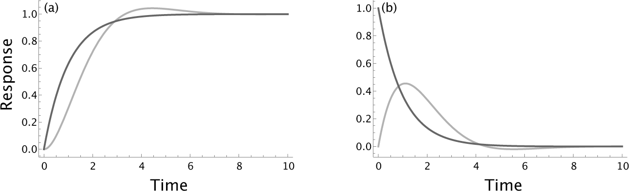
Figure 7.3   Dynamics of the intrinsic process, P, from eqn 7.1, with γ = 1 and optimal parameter $\alpha =\sqrt{1+\gamma }=\sqrt{2}$ (light curves) compared with the optimized open and closed loop systems with process G in eqn 7.7 with $p=1/\sqrt{\gamma }=1$ (dark curves). (a) The unit step response. (b) The impulse perturbation response. From Frank.139

Suppose we take the dynamics of P as known and fixed at the optimum with $\alpha =\sqrt{1+\gamma }$, and find the optimal control process, C. That optimal control process differs between the two architectures because of the distinct ways in which open and closed loops transform input signals.^138,471

However, the best overall internal processing, G, has the same dynamics for both architectures when the control process is limited to a second-order differential equation in its input, r, and output, u. In particular, G is given by¹³⁹

$$ẋ=-p\left(x-r\right),\text{(7.7)}$$

with $p=1/\sqrt{\gamma }$ and final output, y = x. Figure 7.3 compares the dynamics of the optimized process, P, without additional modulation by control (light curves) and with modulating control (dark curves).

The uncontrolled process has reasonably good response characteristics because we chose the parameter α to optimize performance. For γ = 1, the uncontrolled process has performance $\mathcal{𝒥}=\sqrt{2}$. Optimized control improves the response characteristics, yielding an improved performance metric, 𝒥 = 1.

7.3 Error Correction and Signal Amplification

The optimized open and closed loops have the same overall system dynamics in eqn 7.7. However, they construct those dynamics in different ways. The following example illustrates the differences.

STEERING A CAR

Suppose you are the driver, acting as the system’s controller, C. You produce the control signal, u, to alter the control of the car’s internal steering process, P, which sets the car’s direction, y. In other words, you move the steering wheel, which changes the car’s mechanism for setting the direction.

In an open loop, you receive the input signal, r, which is the current direction of the road. In this case, you cannot see the actual direction of the car, as if you were remotely steering a car you cannot see based on the current direction of the road, which you can see.

You move the steering wheel to match the input signal’s direction. You believe the steering mechanism is accurate, keeping the unseen direction of the car on its course. But you cannot check. An inaccurate steering mechanism misaligns the car. You cannot fix that error.

As the input signal about the road’s direction changes, you apply mild pressure to the steering mechanism to adjust its setting for the desired direction. Because you do not know the car’s current direction, you do not know how close or far off you are from matching the car’s direction to the road.

The match depends on how accurately you perceive the road’s direction, how accurately you transform the perceived direction into steering changes, and how accurately the steering mechanism adjusts the car’s direction. The car remains on course only when each step is accurate.

Steering in an error-correcting feedback loop is different. You perceive the input signal, e = r − y, which is the error between the road’s direction and the car’s direction. With information about the error, you steer by adjusting to the error. When the car is too far left, you turn right. When too far right, you turn left.

SIGNAL AMPLIFICATION

The greater the error, the harder you turn. The harder you turn, the faster you correct the error. Put another way, greater amplification of the error signal more rapidly reduces the error. Or, as stated by Åström & Murray [17, p. 320]

Feedback and feedforward have different properties. Feedforward action is obtained by …precise knowledge of the process dynamics, while feedback attempts to make the error small by dividing it by a large quantity.

Dividing the error by a large quantity is equivalent to amplifying the error signal to reduce the error more rapidly. The harder you turn to correct steering errors, the more quickly you reduce the error.

Comparatively, error-correcting systems tend to amplify control signals more strongly than do open loop feedforward systems. The faster a system must reduce errors, the more strongly it tends to amplify error signals. Error correction and signal amplification are among the great principles of systems design.

STABILITY VERSUS PERFORMANCE

Signal amplification causes strong responses, which can make a system prone to instability.

Consider steering. If you are to the left of your target direction and turn hard to the right to compensate, the car may swerve past the target and end up too far to the right. Turn too hard back to the left and you may overshoot again. Overshooting risks instability and total loss of control. Unstable demise is a major risk of error correction with high signal amplification.

The more strongly instability poses a systemic risk, the greater the need for a design to include a margin of safety. Typically, a broader stability margin requires reducing signal amplification and slowing the response to errors. A slower response lowers performance.

7.4 Robustness to Process Uncertainty

In the car example, error correction adjusts for inaccuracies in the steering mechanism. If you are off course because of inaccurate steering, the observed error tells you what you need to do to get back on course.

In general, error correction compensates for variability in process dynamics. Figure 7.4 illustrates error-correcting robustness to process variability for the second-order dynamics of eqn 7.1. In that equation, the parameter, α, determines process dynamics.

As α varies from its optimal value, the performance cost metric, 𝒥, increases. Larger values of 𝒥 associate with greater distance from optimal tracking and thus with worse performance.

Figure 7.4   Sensitivity of open loop (dark curve) and closed loop (light curve) systems to parametric variations in dynamics. The y-axis shows the performance cost metric, 𝒥, and the x-axis shows the process dynamics parameter, α. The optimal value is at $\alpha =\sqrt{2}$, which minimizes the performance, 𝒥. From Frank.139

The figure shows the great sensitivity and lost performance for the open loop without error correction (dark curve). Performance degrades rapidly as α varies from its optimal value. Open loop control cannot compensate for the misspecification of process dynamics.

The performance of the error-correcting process degrades relatively little with variation in process dynamics (light curve). In that case, the constant input of the error between the target output and the actual output allows the system to improve its performance without prior information about system dynamics.

Robust design in life and in human engineering would not be possible without error correction. Building and maintaining precise components are very costly and perhaps impossible. With error correction, systems can perform robustly with sloppy components and limited information.

THE PARADOX OF ROBUSTNESS

The ultimate effect of shielding men from the effects of folly, is to fill the world with fools.

—Herbert Spencer

The better a system becomes at compensating for perturbations and errors, the better the system can handle imprecise and erratic system components. System robustness weakens the selective pressure acting on the system’s components. Weaker selective pressure on the components leads to decay in their performance.

Overall, the more robust a system, the more the system’s components will tend to decay in performance. Better error correction begets more errors.^124,125,134

Component decay may take the form of increased variability or sloppiness in function. Alternatively, weaker selective pressure on components may cause them to decay to less costly and lower performing designs. In the latter case, the economics of efficiency favors robust systems to use cheaper components.

Comparatively, the better a system is at buffering fluctuations in its components, the more the components will tend to accrue genetic variability^349,427,435 and stochastic variability in expression, and the more those components will tend to decay to cheaper, lower performing states.¹²⁵

Within systems, performance will be more sensitive to some components than to others. The less sensitive the system is to fluctuations in a particular component, the more variable and lower performing that component will tend to be.¹⁴⁰

In theory, the paradox of robustness should be a ubiquitous aspect of control systems. If so, the paradox likely plays a key role in biological design throughout the history of life. However, this aspect of design has received little attention in theory or application.

7.5 Responsiveness versus Homeostasis

Microbes must respond to environmental change. When a new food source arrives, cells change to acquire and digest the food. Faster response of the required traits typically provides a benefit.

Microbes must also maintain steady expression levels in a stable environment. Homeostatic maintenance poses a challenge because environmental signals often fluctuate significantly over short time periods. Slower response to changing signals typically improves homeostasis.

Overall, fast response improves tracking of true environmental change, whereas slow response improves homeostatic maintenance relative to noisy environmental fluctuations. This tradeoff between responsiveness and homeostasis shapes many aspects of design.89,138,303,471 Figure 7.5 illustrates the tradeoff.

Figure 7.5   The tradeoff between responsiveness and homeostasis. Smaller performance values correspond to better performance. The parameter γ from eqn 7.6 determines the relative weighting between responsiveness to an environmental change and the ability to maintain a homeostatic setpoint when perturbed by a single large impulse disturbance. Larger γ weights homeostatic performance more heavily. The different curves in each panel show different costs, ρ, for the control signal, u. The control signal penalty, given as log₁₀ρ, is  − 4 (light line),  − 2 (medium line), and 0 (dark line). (a) Responsive performance to a step increase in the environmental input signal, measured by 𝒥_s in eqn 7.4. (b) Homeostatic performance in response to an impulse perturbation in the environmental input signal, measured by 𝒥_p in eqn 7.5. Redrawn from Frank,139 which also provides details on the assumptions and the optimization methods used to obtain the curves.

All curves arise from minimizing the performance metric in eqn 7.6, repeated here for convenience,

𝒥 = 𝒥_s + γ𝒥_p.

The first component, 𝒥_s, is the total distance between the system’s output value and the recently shifted target value caused by a long-term environmental change. Smaller values mean closer tracking of the environment and more successful performance.

The second component, 𝒥_p, is the total distance between the system’s output value and its homeostatic setpoint. At time zero, the system receives a large instantaneous environmental impulse, which then immediately disappears. The impulse perturbs the system from its setpoint. Greater perturbed deviation and longer time of return to the setpoint increase 𝒥_p. Larger performance values associate with worse homeostatic maintenance and less successful performance.

The parameter γ determines the relative weighting between the two components of performance. Larger γ weights the homeostatic component more heavily.

Figure 7.5a shows the responsiveness component of performance. The performance value rises and success declines as γ increases because a stronger weighting of homeostasis reduces responsive success. In essence, the system responds more slowly, protecting homeostasis from being perturbed by fluctuations but simultaneously slowing the system’s ability to respond to real change.

Figure 7.5b shows the opposing change in homeostatic performance. Larger γ values weight this component more strongly, favoring lower (better) performance values.

The different curves in each panel of the figure correspond to different cost weightings, ρ, for the control signal, u. As ρ rises, control signals become more costly. In this example, responsiveness requires a stronger control signal than does homeostasis. As the cost of the control signal rises, responsiveness becomes relatively expensive, altering the balance of the system toward favoring homeostasis over responsiveness.

The tuning of system design for responsiveness versus homeostasis also depends on the frequency spectrum of environmental change. When environments tend to change slowly, at low frequency, systems gain by being more responsive to altered conditions. When environments fluctuate rapidly, systems gain by improving homeostasis, which typically means that they respond more slowly to change.

Put another way, as systems become better at coping with high-frequency noise, they often degrade in the speed of their response to longer-term changes. Alternatively, as they become better at responding rapidly to change, they become more sensitive to short-term perturbations that disrupt homeostasis.

One can plot a system’s response to different frequencies of inputs. Such Bode plots play a central role in engineering control design.^{89,138,303,471} How can one tune a system to be more responsive to certain input frequencies and less sensitive to perturbations at other frequencies? And, comparatively, how does a change in responsiveness at particular frequencies alter the predicted mechanistic attributes of trait design?

7.6 Sensors

Matching the environment requires external sensors. Maintaining homeostasis requires internal sensors.

Sensor design raises several challenges. What frequencies of environmental change provide useful information? What frequencies should be ignored? Typically, low-frequency signals represent long-term environmental changes that require adjustment. High-frequency fluctuations represent noise that should be ignored.

Each sensor has a particular response profile to different frequencies. How best to tune frequency response? Mechanistically, how are sensors built from biological components?

Sensors can be thought of as estimators of parameters given some data. Optimal estimation often follows from analysis of Fisher information, a way of quantifying the information in data about a parameter of a probability distribution.44

That information abstraction only gives a hint about the many problems of sensor design. Individual sensors necessarily have particular frequency and magnitude sensitivities. Given variable sensor sensitivity, what is the best design of sensor arrays to meet particular environmental challenges?^137,196

What is the best temporal and spatial deployment of sensors? How does one balance the benefits of information versus the costs of sensors and the use of the acquired information?

Comparatively, as the frequencies of meaningful signals change, how does sensor design change? How does a change in the magnitude of key signals alter sensor design?

Sensors provide a great challenge in the study of biological design. A broad comparative theory has yet to be developed. Only through comparative predictions can one study the forces that shape design.

7.7 Control Tradeoffs

This chapter emphasized tradeoffs in the regulatory control of trait expression.139,140

OPEN LOOP VERSUS ERROR-CORRECTING CLOSED LOOP

Error correction provides benefits when a system does not have perfect information about disturbances and dynamics. By measuring the error between the target output and the actual output, a system can continuously adjust itself to improve performance. It can also compensate for sloppy or faulty components.

Error correction requires additional sensors to measure the error and strong signal amplification to reduce the error. Simpler open loop control may be better when a system has good information about its dynamics or the costs of error correction are high.

Comparatively, error correction is more strongly favored as information about dynamics declines, perturbations increase, or components become less reliable. In other words, robust design becomes more strongly favored as dynamics become less predictable.

ROBUSTNESS AND DECAY

The more robust an error-correcting system becomes, the more component performance tends to decay. By correcting for variable or faulty components, error correction reduces the benefit of precise and highly optimized components. As the benefit and associated force favoring component performance declines, the components tend to decay to lower cost and lower performance. Components may also become more variable in their output. Robust system design may often lead to highly stochastic system components.

PERFORMANCE VERSUS STABILITY

High performance often means adjusting quickly to a changed environment. Fast adjustment requires a strong force in the direction of the new target. The stronger the force, the more rapid the adjustment and the greater the chance of overshooting the target. Overshoot requires a strong countering force to reverse direction. Overshoot in the opposite direction may occur.

Increasingly larger overshoots cause instability. Typically, the danger of instability rises with the speed of adjustment. To prevent dangerous and potentially lethal instability, systems may pay the cost of reduced performance in order to lower the risk of instability. The greater the margin of safety is, the lower the average performance will be.

Comparatively, environments that impose greater perturbations favor systems designed with greater stability margins and lower average performance.

RESPONSIVENESS VERSUS HOMEOSTASIS

Systems must respond to long-term environmental change and avoid being perturbed by short-term noise. These goals of responsiveness and homeostasis often trade off against each other. A more responsive system adjusts rapidly to environmental change. But a system that responds quickly is sensitive to rapidly fluctuating false signals.

Comparatively, noisier environments favor greater homeostasis at the expense of responsiveness. By contrast, dominant low-frequency environmental changes favor greater responsiveness. Greater cost of control typically favors homeostasis over responsiveness because a responsive design tends to require costly internal signal amplification to track environmental change.

SENSOR DESIGN

The theory of sensor design requires greater development. Some obvious tradeoffs arise. In sensor arrays, more low quality sensors trade off against fewer high quality sensors. Greater numbers of sensors provide better spatial coverage. Combining inputs from multiple sensors may require more cost to compute the output signal from the multiple inputs.

When tuning sensors, what factors favor particular frequency bands of sensitivity and particular magnitudes of sensitivity? What is the best combination of sensitivities in an array? Mechanistically, how do cells achieve sensor designs with particular functional attributes? Comparatively, how do changes in environmental parameters alter sensor design?