This appendix describes the major data sources used in the calculations, graphs, and maps throughout the book.
The climate classification used in this book is the Köppen-Geiger system, which classifies the major world climate zones into five main categories based on temperature and precipitation, and a sixth (highland) category based on elevation.
Summary of the Köppen-Geiger Classification system
| Type |
Description |
| A |
Equatorial climates |
| Af |
Equatorial rainforest, fully humid |
| Am |
Equatorial monsoon |
| As |
Equatorial savannah with dry summer |
| Aw |
Equatorial savannah with dry winter |
| B |
Arid climates |
| BS |
Steppe climate |
| BW |
Desert climate |
| C |
Warm temperate climates |
| Cs |
Warm temperate climate with dry summer |
| Cw |
Warm temperate climate with dry winter |
| Cf |
Warm temperate climate, fully humid |
| D |
Snow climates |
| Ds |
Snow climate with dry summer |
| Dw |
Snow climate with dry winter |
| Df |
Snow climate, fully humid |
| E |
Polar climates |
| ET |
Tundra climate |
| EF |
Frost climate |
| H |
Highland climates (varied) |
Source: Markus Kottek, Jürgen Grieser, Christoph Beck, Bruno Rudolf, and Franz Rubel, “World Map of the Köppen-Geiger climate classification updated,” Meteorologische Zeitschrift 15, no. 3 (2006): 259–63. https://doi.org/10.1127/0941-2948/2006/0130.
The Strahler and Strahler map, in turn, is based on:
R. Geiger and W. Pohl. 1954. Revision of the Köppen-Geiger Klimakarte der Erde Erdkunde, Vol. 8: 58–61.
Since the climate has changed over time, projecting today’s climate map back to conditions of past millennia is only an approximation.
Population Data
Historical Population Data
Much of the historical population data draws on Kees Klein Goldewijk, Arthur Beusen, and Peter Janssen’s study on the HYDE 3.1 project data. The study estimates “total and urban/rural population numbers, densities and fractions (including built-up area) for the Holocene, roughly the period 10000 BCE to AD 2000 with a spatial resolution of 5 min longitude/latitude.” Details may be found here:
Kees Klein Goldewijk, Arthur Beusen, and Peter Janssen. “Long-Term Dynamic Modeling of Global Population and Built-up Area in a Spatially Explicit Way: HYDE 3.1.” The Holocene 20, no. 4 (2010): 565–73. https://doi.org/10.1177/0959683609356587.
World population, GDP and per capita GDP from 1–2008 CE
The historical economic data draw on the Maddison Project Database. While this database has been adapted and updated during the last decade, I chose to use the 2010 release version as it provides the most comprehensive coverage by countries, regions and years. The 2010 dataset was the final version provided by the late economic historian Angus Maddison himself, covering world population, GDP and per capita GDP from 1 to 2008 CE. For further information on the project see:
Maddison Project Database, version 2010. Jutta Bolt, Robert Inklaar, Herman de Jong and Jan Luiten van Zanden (2010), “Rebasing ‘Maddison’: new income comparisons and the shape of long-run economic development,” Maddison Project Working paper 10
Gridded Population Data for 2015
The spatially explicit population data for 2015 is from the Center for International Earth Science Information Network (CIESIN) Columbia University. 2016. Gridded Population of the World, Version 4 (GPWv4): Population Count. Palisades, NY: NASA Socioeconomic Data and Applications Center (SEDAC). http://dx.doi.org/10.7927/H4X63JVC.
Ancient Cities data
The data on ancient cities is based on Meredith Reba, Femke Reitsma, and Karen C. Seto,“Spatializing 6,000 Years of Global Urbanization from 3700 BC to AD 2000,” Scientific Data 3 (2016): 160034. https://doi.org/10.1038/sdata.2016.34. I deeply thank Dr. Reba for assistance in accessing these very insightful data.
Data Used in the Creation of Maps and Geospatial Analysis
The maps draw on shapefiles from the following sources.
Coastal and river boundaries:
Made with Natural Earth, naturalearthdata.com. (Note that I apply present data coastal and river boundaries to ancient civilizations. This is of course only an approximation in view of changes in coastlines and river flows.)
Ancient Empire/Regional outlines:
Figure 5.2 Empire of Alexander the Great
Figure 5.3 Roman Empire
Figure 5.4 Han Dynasty
Figure 5.6 Map of Silk Road
Figure 5.8 Umayyad Empire
Figure 5.9 Ottoman Empire
Figure 5.10 Song Dynasty
Figure 5.12 Timurid Empire
Throughout the text, I refer to seven continental regions, Africa (AF), Asia (AS), Commonwealth of Independent States (CIS), Europe (EU), Latin America (LA), North America (NA), and Oceania (OC). Note that for purposes of analysis, the CIS is separated from Europe and Asia, but in standard geographical accounts would be part of those two continents.
Following are supplementary tables that contain calculated data referred to in the text.
Table 1.3a Percent Land and Population Within 100 km of Coasts
Table 1.3b Percent Land and Population Within 20 Km of Rivers
Table 1.3c Percent Land and Population Within 20km Rivers and/or 100km of Coast
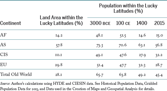
Table 3.1 Percent Land Area and Population Within the Lucky Latitudes (Old World)