7
Issues with BEM

Introduction

The typical opening for literature dealing with performance issues in architecture would highlight the importance of statistical data in order to save energy in the building sector while emphasizing that there is room for improvement. Such approaches usually continue by delving into the opportunities opened up by new simulation technologies and mention the hardships and costs of the technical management of informing design decisions with performance data.

All of these issues are very real and true, yet there is another aspect omitted: the design appeal of the approach itself. To provide some context, it is possible to refer to the widely accepted rule that energy modeling in the early stages is more effective than energy modeling in the later stages. This rule leads to the simple-box modeling approach that can be helpful for architects—so helpful, in fact, that the current research easily falls within the same boundary. But at the same time, the simple-box approach is simplistic in the sense that the simple-box itself can be engulfed in the sea of decisions that comprise a building’s design. It may also be unfair to call such design performance-based, as the degree to which performance plays a role may not be that great. As a result, the risk is reducing performance-based design to a parametric shading or a simple simulation that is not nearly as exciting as the other available alternatives in the digital age.

Designing based on performance, however, can be both very exciting and very complicated. In the theoretical context of avoiding the architect as master creator, making design decisions based on styles or ideological allegiances and in general imposing a subjective will on the material,¹ performance-based design can be used to generate new and even unpredictable forms.

The advent of advanced computation, in other words, means that the conceptual and engineering aspects of architecture can stand in agreement with each other; or performance aspects need no longer be external to the building design and form making. Would the architectural community support pushing performance-design to its extremes to achieve the optimal form? Maybe because such design includes a loss of control on the part of the architects, or perhaps this process involves a certain level of idealism, but it is also because the phrase the optimal form lends itself to varying interpretations. However, if other designers are curious to know or define what these versions of the optimal can be, there are still a few obstacles to overcome.

This chapter locates some of these obstacles to defining the optimal while also suggesting ways around them. In other words, our objective is to achieve a malleable methodology to evaluate and optimize the performance of geometries in a holistic framework.

WBEM Obstacles

A relatively new user might hear about the whole-building energy model (WBEM) and be excited about the ease with which a certain software package can execute such analysis. As logical as that expectation might be in the digital age, however, in reality (at least up to now), no software actually offers such a whole-building analysis, and there is not even a clear-cut methodology for such a process! One reason is that many buildings are too complex to simulate as a whole; thus, the whole is broken into pieces, each simulated separately and then pieced back together within the reporting results. Here, on the one hand, neglecting certain aspects of energy consumption may occur in the process, creating an effect on the overall resultant performance-based form. On the other hand, within a WBEM methodology— usually called one parameter at a time optimization—a certain linearity replaces the actual complexity of the system.

To state it more clearly, at times no parameter has primacy over the others, and choosing one particular parameter by which to start affects the result. In this milieu, the most relevant example is probably lighting. By giving a certain primacy to thermal optimization, as is the case with current WBEM, the modeling process postpones the lighting calculation, effectively omitting it from consideration. A real WBEM optimization, however, should synchronize the involved factors and account for the actual complexity of the system—at least to the extent that it is possible.

Lighting

The omission within most WBEM frameworks is the dynamic and differential effect of the sun and solar gains, flattening lighting power density (LPD) into a single number. LPD considers only the building function and the total area, and does not reflect on the building geometry, the window shape and size, or numerous other relevant aspects of the building. For lighting energy use, LPD is the default calculation in most software packages; because LPD allows quick calculations it is possible to produce numerous results and iterations (Figure 7.1). Since the floor areas and building volumes are equal across the range, so too is the resulting lighting electricity consumed.

By ignoring the daylight that penetrates through the windows, the WBEM calculation is primarily thermal-based. While this might have its own applications, it represents and emphasizes only one set of forces, which drives the geometry toward a more compact and less transparent shape. The logical result, as Figure 7.1 shows, may end up being a square plan with the lowest WWR (window-to-wall ratio).

The geometry discovered from thermal influences protects the core of the building and results in relatively poor lighting. In reality, however, daylighting forces drive geometries toward a narrower and more transparent result. The narrowness may occur in the plan or in the section (such as in towers with multiple floors in comparison to a bulk single-floor plan with the same area), but in general the floors are pushed closer to the windows and a larger part of them is exposed to daylight. As one can see, thermal and lighting forces are opposed, and this presents designers with exciting opportunities to experiment with different formal strategies for locating the sweet spot where the building’s thermal and lighting needs optimally balance each other.

Thus, one can expect within a WBEM a unifying framework in which the energy consumed by electric lighting and the energy needed for thermal purposes can merge into a whole unit. As mentioned earlier, the main obstacle here is that research on lighting—while advancing quickly and introducing a new wave of dynamic metrics—moves separately from the other building metrics, meaning that there is therefore no unanimously accepted methodology for a whole-building energy analysis. Before proposing a solution, we should briefly examine some different aspects of this problem:

• Lighting research introduces dynamic metrics (such as spatial daylight autonomy (sDA) and annual sunlight exposure (ASE)) that do not directly address energy consumption. The latest manual (IES LM-83-2012), for example, avoids the problem, saying only that “electric lighting management is highly variable.”²
• Transforming the lighting metrics into energy units includes esoteric assumptions and decisions that may not be convenient (or at least might not be the main concern) for architects involved in the early stages of design.
• Lighting calculations are complicated and much slower than thermal ones. Hence, when synchronizing the two, one should expect a lower resolution in any BFM or evolutionary algorithm. Cloud-computation technologies may be helpful in this regard, but uploading and downloading iterative data and working within networking frameworks has its own challenges.

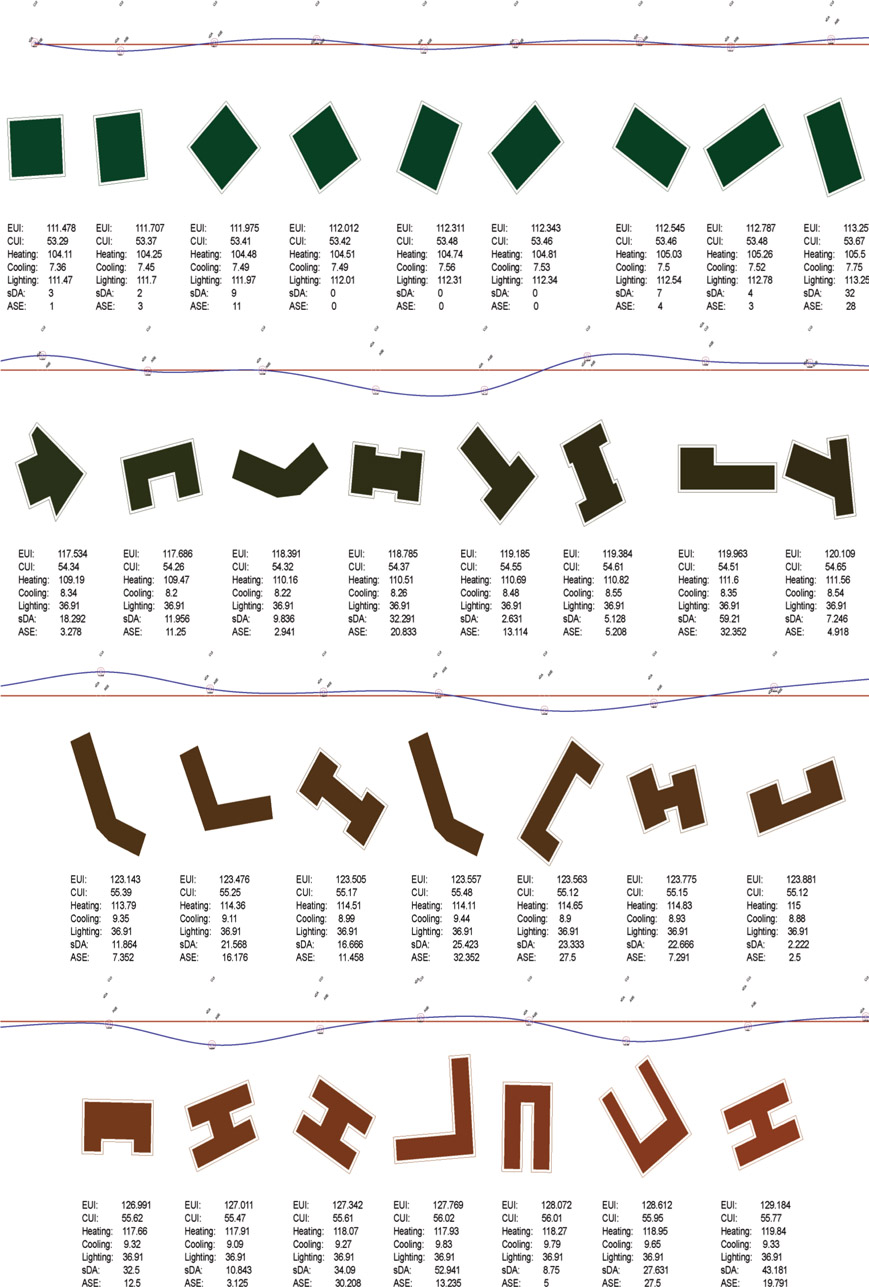
Figure 7.1 Whole-building energy analysis using LPD for the lighting energy consumption

Parallel Example (Literature Review)

As expected, because dynamic lighting metrics are relatively new, the available literature is thin. Designers and computation experts, however, are gradually facing the problem of dynamic lighting metrics more often, and one may expect further developments in the near future. A recent example is the work of Kyle Konis’s team, which refers to the problem of synchronizing thermal lighting calculations³ and recommends using a new metric, spatial useful daylight illuminance (SUDI).⁴ To synchronize the results they suggest that the values should be “scaled to the same numerical range (e.g., 0–100).”⁵

While the gap in the existing knowledge (i.e., a method of synchronizing thermal and lighting results) may legitimize radical solutions such as inventing a new metric, this new methodology still leaves the transformation from metrics of daylighting to units of energy undetermined. In other words, remapping and adding the results of thermal calculation (which is an energy metric) and lighting calculation (which is a percentage value) is not accurate, and does not reflect the actual building’s performance. This movement from lighting metrics to energy metrics includes more assumptions and decisions that remain undiscussed and unresolved.

Methodology

The main element of the current methodology is to avoid closing the space of discussions or arguing for a single correct answer. Instead, in the following pages several methods and their results are placed next to one another to provide extensive information on this issue. Before getting into the technicalities, defining these main approaches can be helpful:

LPD: As mentioned previously, lighting power density is an ineffective way to ascertain a building’s lighting needs. However, the metric will be provided to establish a baseline. Because the total floor area and the building functions remain the same across each group of iterations, the LPD value will remain constant.

Dimming schedule: A conventional way to adjust a building’s lighting power consumption is to inform it with a lighting calculation based on climate data (also known as climate-based in DIVA). Based on a predefined set point (target illuminance level), photo-sensor-controlled dimming will provide a schedule that defines whether lighting switches are on or off in a given area at a given time over the course of the year. The dimming system itself consumes some energy (referred to as standby power and ballast loss factor) that should be included. Thus, if an area has sufficient illumination, the building’s dimming system will reduce energy consumption by turning off the lighting in that area.

Reduced LPD: Compared with the previous option, reduced LPD requires both a prior lighting calculation and the sDA number produced. Using the sDA number to modify the LPD number reflects the possibility of using natural light. This approach is a practical solution that is fast and useful, and was suggested first by the Sefaira team.⁶ Equation 7.1 shows the formula used, which is also simple:

$$\mathrm{Reduced}\mathrm{LPD}=\left[\right(1-\mathrm{sDA}∕100)\times 0.8+0.2]\times \mathrm{main}\mathrm{LPD}$$

(7.1)

sDA-based lighting (lux deficiency method): This method is specific to the current research and is suggested by the author, hence, it requires a bit more explanation. It makes use of the basic structure of sDA calculation as depicted in Figure 7.2.

sDA is calculated based on a grid of sensors. At a certain sensor, if the lux level is above the threshold (300 lux is currently the only threshold endorsed by the Illuminating Engineering Society [IES]), there is no need for artificial lighting and the power consumption would be zero. However, if the lux level is below the threshold—say, x = 250—the artificial lighting needed should provide threshold – x, or 300 – 250 lux at that specific point, yielding a result of 50 lux. The sDA calculation also predefines the grid size (or more specifically, its area), and so the only missing bit of information is the lighting type. By determining the lighting source, it is possible to obtain the luminous efficacy (lm/W). Regular numbers in Table 7.3 show luminous efficacy for lighting types, but note that it is possible to use a mixture of different types to achieve different results.

With the available information (i.e., the extra illumination needed [in lux], the area, and the lighting type) it is possible to calculate the needed electrical energy at a certain point on the grid. The power P in watts (W) is equal to the illuminance E_v in lux (lx) times the surface area A in square meters (m₂) divided by the luminous efficacy η in lumens per watt (lm/W),⁷ shown in Equation 7.2:

$$P=E_{\mathrm{v}}\times A∕\eta$$

(7.2)

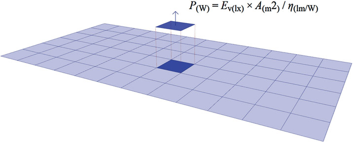
Figure 7.2 Diagram showing how to move from the sDA metric to energy consumption.

Of course, the total lighting consumption would be the cumulative sum of the values across all of the sensors in the grid over time. Similar to the dimming schedule option, this approach should consider a consumption value for the control and distribution system. In any case, however, the internal consistency achieved across all of the iterations should be sufficient for both evaluating energy performance and defining energy optimization goals.

Table 7.3 Luminous efficacy for common lighting sources.

Lighting type	Luminous efficacy (lm/W)
Tungsten incandescent light bulb	15
Halogen lamp	20
Mercury vapor lamp	50
Fluorescent lamp	60
LED lamp	60
Metal halide lamp	87
High pressure sodium vapor lamp	117
Low pressure sodium vapor lamp	150

IES defines sDA as the “asset value of daylight sufficiency”;⁸ and this method is based on using the lux deficiency to calculate the necessary energy. In returning to the difference between daylight autonomy (DA) and continuous daylight autonomy (CDA), we find a similar situation; sDA cuts the results at 50 percent, meaning that 49 percent and 51 percent suddenly become very different. The lux deficiency method, however, calculates the extra illumination needed for the points that do not meet the requirements, and thus provides a more distributed result similar to CDA. In this method, 49 percent and 12 percent are both failing numbers, but the energy needed to compensate for the lack of illumination is different in each case.

As a final note, and to put these methods in their contexts more properly, it is worth mentioning that the first two, namely LPD and the dimming schedule, were used even before the dynamic metrics (such as sDA) were available, which is probably why they are still widely used. LPD is in fact independent from any actual lighting calculation and the dimming schedule method can be produced by traditional types of climate based analysis—for example the conventional DA (daylight autonomy). The new dynamic metrics, however, may require new methods for the calculations as well. Reduced LPD and Lux deficiency methods are, accordingly, the attempts at embedding the lighting calculation within the processes and loops of the sDA procedure, both for consistency and for saving time.

Preparation

In general, the current research is an attempt to align as closely as possible with sDA/ASE, and many of its aspects are accordingly defined by those metrics. For example, the goal of the process discussed in this chapter was to engage with a wide range of possibilities, including different climates, geometries, types, and sizes. It would then make sense to use different types of workspaces with different illuminance thresholds, especially in spaces with decidedly disparate visual tasks or illuminance needs such as warehouses, office spaces, or healthcare facilities. But IES LM-83-12 “does not have a research basis for recommendations for such areas”⁹ yet, and as such, using different illuminance thresholds with such disparate workspaces would be viewed as coming far too soon. Therefore, under the title of office space, only a single building type with a threshold of 300 lux is studied. Some of the variables, however, include:

Building size: Three different office size categories are analyzed in Table 7.4, essentially using the prototypes by the U.S. Department of Energy.

Climate: Choosing several climates in the U.S., the simulations used four cities (New York, New York; Omaha, Nebraska; Phoenix, Arizona; and Miami, Florida) to represent four different conditions and determine how climate affects the results.

Geometry: A letter-shape strategy was used in which shapes were categorized into different groups: L, T, O, H, U, and trapezoidal. Such forms are functional, but are at the same time not overly simplistic, establishing a middle ground between pure simple-box modeling and complex agent-based formal strategies. Windows distribution was equal over all sides (walls). If the total square footage of the building is lower than 25,000 ft² (2,322.576 m²), a WWR of 25 is used. For larger buildings, the WWR would be 30. It might make sense to have a larger window on the south or north side; the aim here is not to optimize the form but rather to show the performance behavior of changing forms. Across each of the iteration groups (small, medium, and large) created here, the total square footage and volume remain constant so that the geometries continue to be comparable. The floor to floor height also changes as we move toward larger offices, from 3 m for the small and medium shapes to 5 m, therefore studying each group separately (i.e., small offices against small offices, and not against large or medium offices) makes more rational sense.

Materials and conditions: Better material generally leads to better performance. Accordingly, in this study, materials remain unchanged in the hope that the focus will shift toward geometry and design. Keeping the two completely separate is not possible, because as surfaces such as roofs or walls change in different iterations, the material composition of the building changes as well. That being said, the items listed in Table 7.5 remain consistent across all of the iterations in this study.

Table 7.4 Typical office sizes evaluated in simulations.

Office size	Area (ft2)	Area (m2)	Floor to floor height (m)	Number of floors
Small	5,000	464.5	3	1
Medium	50,000	4,645.1	4	1-3
Large	500,000	46,451.5	5	1-12

When synchronizing thermal and lighting simulations, another issue, material consistency, is of high significance. Material consistency is more important when dealing with transparent items, i.e., windows. If selecting a specific window for the building, one should use both the thermal and lighting properties from that same window’s materiality. This process might not be—and usually is not— automated, and requires some extra attention. Table 7.6 lists examples of different properties that come with common window types.¹⁰

Table 7.5 Constant items for simulations.

Material/condition	Value
Walls	R = 30
Floor	R = 20
Roof	R = 80
Window	U = 1.32 W/m2K
Heating set point	21.66 °C (71 °F)
Cooling set point	24.44 °C (76 °F)

Table 7.6 Material consistency for thermal and lighting calculations.

Material	SHGC	U-factor (W/m2K)	Visual transmission %	Visual transmissivity (RGB) %
Glazing SinglePane 88	0.82	5.82	88	96
Glazing DoublePane Clear_80	0.72	2.71	80	87
Glazing DoublePane LowE 65	0.28	1.63	60	71
Glazing DoublePane LowE Argon 65	0.27	1.32	65	71

Analysis period: Similar to the problem of building type—which is limited to only one—here again there are limitations imposed by IES LM-83-12. According to the manual, “the period of analysis is fixed at 10 hours per day, from 8AM to 6PM local time,” which “results in 3,650 hours for a complete annual analysis.”¹¹ While this limitation excludes schools or other buildings with varying schedules, for now, the insistence on unifying buildings with such disparate schedules forms a necessity “for specification and reporting so that comparisons can also be made to a consistent performance standard.”¹²

Analysis grid: Admittedly, and as Figure 7.7 shows, changing only the grid size while keeping all other factors constant does indeed affect the result. Thus, to report a consistent performance standard, one should use the grid suggested by IES LM-83-12. However, that grid (24′) requires too many sensors, especially for the large offices (500,000 ft²). Because of the limitations in calculation power, the grid sizes shown in Table 7.8 were used. Other aspects of the grid based on IES LM-83-12 are a threshold of 300 lux (27 foot-candles) and a height of 0.8 m.

Figure 7.7 The effect of grid size on analysis results.

Table 7.8 Grid sizes.

Building size	Grid
Small	3 ft (0.9 m)
Medium	4 ft (1.2 m)
Large	8 ft (2.4 m)

Software Details

The entire study was conducted inside Rhinoceros (a NURBS modeling tool). Geometries are exported as meshes to Grasshopper (GH). To perform the iterative study, GH and a Python script were used, though the most important package was DIVA v3 for GH, which provided the links to EnergyPlus and Daysim for thermal and lighting calculations, respectively.

Furthermore, sDA works paired with ASE. For that reason, two separate daylight analyses are performed, one with six bounces and the other with zero. The six-bounce version has a threshold of 300 lux, and the zero-bounce version has a threshold of 1,000. The only benefit of calculating the sDA number by computational programming is that calculating lux deficiency and sDA can occur within the same loop, saving a bit of calculation time. In other words, if illuminance at a certain sensor is above 300, it qualifies to be added to the temporal dimension of sDA. Later, one should test whether this is above or below 50 percent of the schedule, and if not, it is possible to calculate and accumulate 300 – x, which gradually builds up the total deficiency.

The thermal component is a simplified single-zone analysis in which the whole building is one zone—internal floors used for lighting calculations are nonexistent in the thermal calculations. The modified LPD value, or the dimming schedule, is then passed to the thermal component to complete the analysis. For the lux deficiency method, LPD = 0 is used, and the result of the light calculation (electricity, as expressed in kWh) generates the source energy and the carbon emissions.¹³

Visualization of Results

While it is possible to use genetic algorithms to optimize the form based on predefined goals, using a strategy closer to brute force in this study helped to organize the results based on the total energy consumption. This is because in packaged genetic algorithms, the process remains undisclosed and only the results are visible; however, with BFM it is possible to observe how factors such as ratio, orientation, and the others evaluated affect the behavior of forms in relation to energy consumption.

Figure 7.9 sDA color-coding example.

Figure 7.10 Binary sDA.

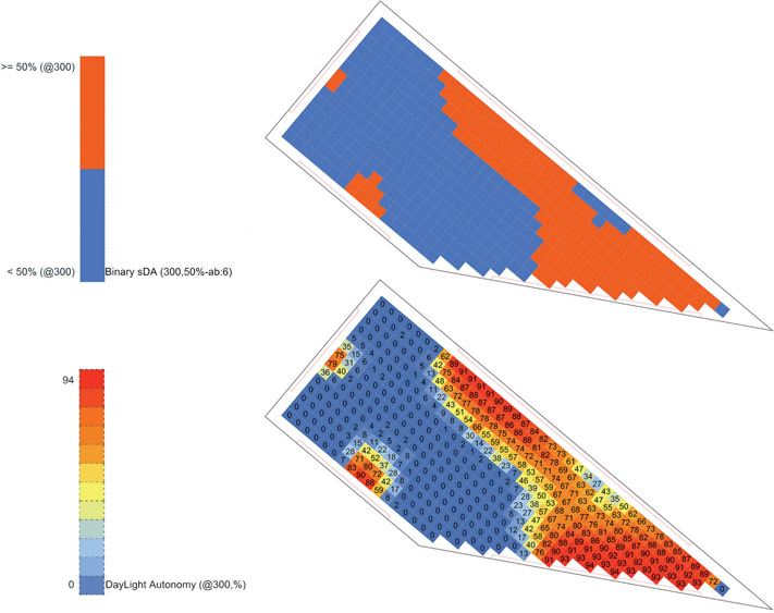
Using a particular visual style helps to provide clear information. For example, as Figure 7.9 shows, sDA itself is just a number that may work in comparison with other buildings and their sDA values, but it does not disclose much information about the building. For this reason, in the current study the results report a visual style called binary sDA. Figure 7.10 shows an example of binary sDA.

The process in Figure 7.10 is simple; the lower figure shows a sDA with the threshold of 300 lux and the upper figure shows whether or not that value is above 50 percent. At the same time, based on the brighter part of Figure 7.10, the sDA value is visualized.

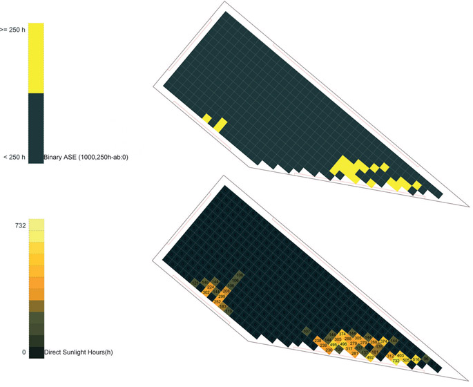
The other style is binary ASE, depicted in Figure 7.11. Here, the lower image demonstrates the number of hours that a certain area is exposed to direct sunlight, and the upper image shows whether or not the time of exposure to direct sunlight is above 1,000 hours per year. Again, in this picture one can also observe the ASE value. Finally, as Figure 7.12 shows, graphing key metrics of the buildings compare each result to provide additional insight into the behaviors of the forms.

Figure 7.11 Binary ASE.

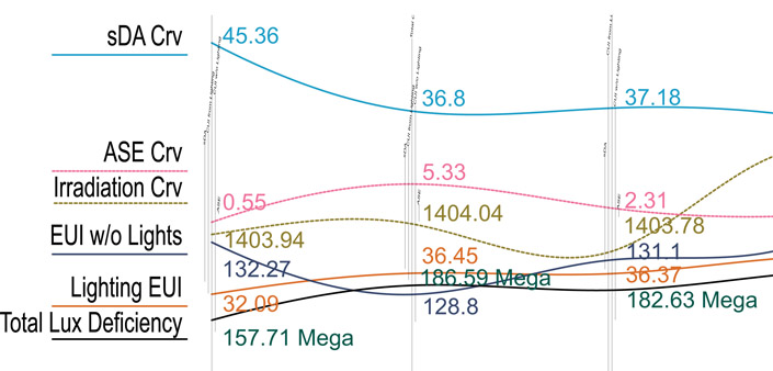
Figure 7.12 Line graphs showing the behaviors of each iteration of the building simulation.

Pattern Guide

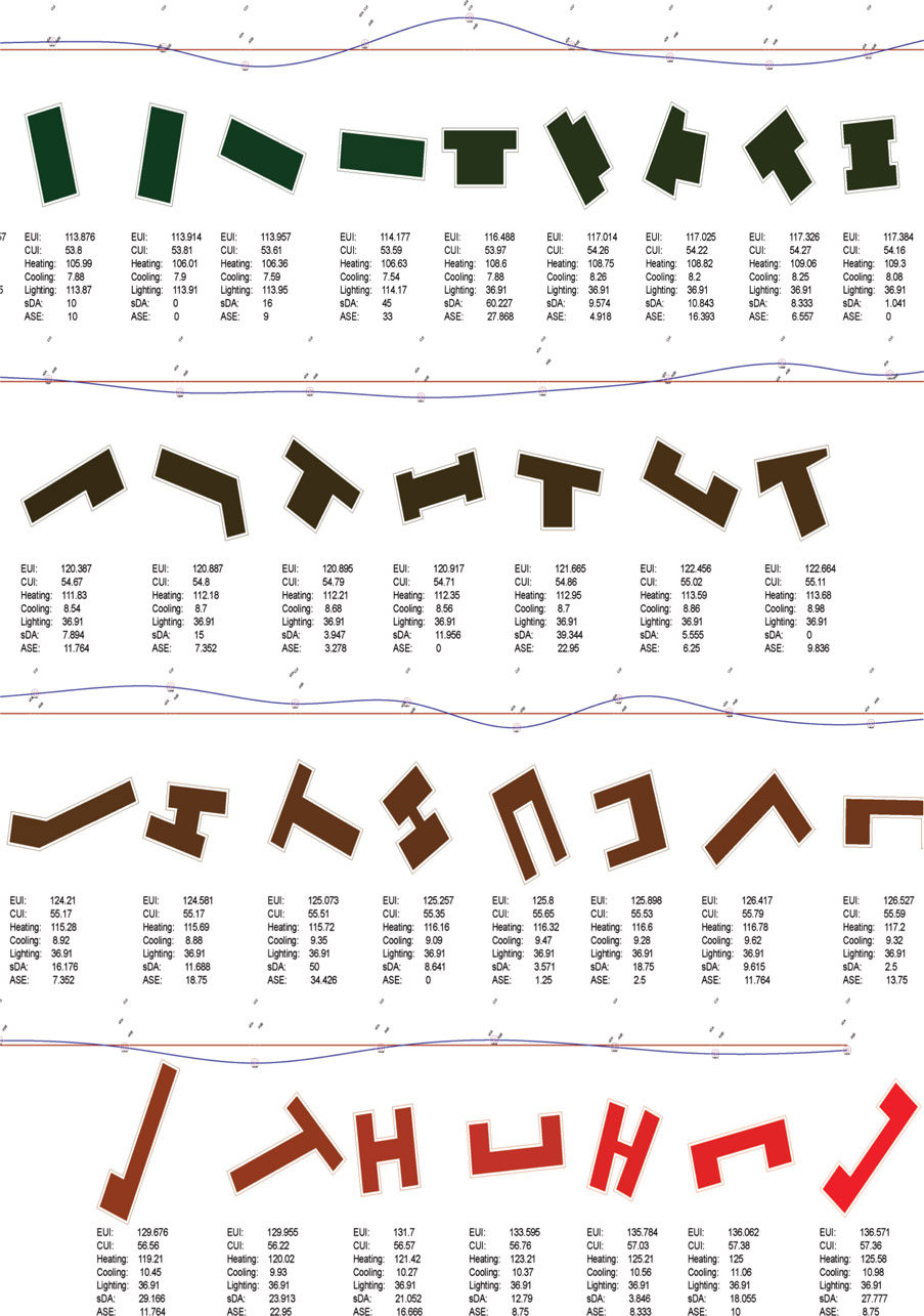
In this truer WBEM study, the following pattern guide (Figures 7.15–7.38) demonstrates the results of the research integrating lighting energy into the WBEM geometric building variations. Each building is modeled and simulated in isolation; therefore, no shading from context is included and the number of iterations depicted are limited because they are bound to the print size. Nevertheless, our hope is that the methodology and information provided here may prove useful to those involved in performance-based design.

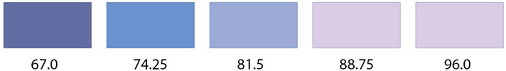
Table 7.13 shows the range of locations and building sizes included. Described in Figure 7.14 are the color scales used. Since each simulation produces its own high-to-low range, numerical comparison is only possible within each shape and location, not across ranges. For example, a good EUI in Omaha for a small H-shaped office is 40 kBtu/m²/yr, whereas the good EUI of a large H-shape in Phoenix is 240 kBtu/m²/yr. Therefore, each shape, location, and size presented in the pattern guide can only be compared within similar sizes or cities. Figures of small offices are at a 1:100 scale. The medium and large offices are at a 1:300 and 1:500 scale respectively. Given range of resultant geometries, as consistently as possible each shape type is presented, albeit a bit differently.

Table 7.13 Outline of locations and office sizes shown in the pattern guide. Letter shapes of H, L, T, and U, including trapezoids (Trap), were randomly mixed and selected based on their performance results. Items noted with “X” identify cities where small, medium, and large shapes are present in the pattern guide.

Office size	Miami	New York	Omaha	Phoenix
Small	X	X	X	X
Medium	X	X	X	X
Large	X	X	X	X

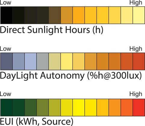
Figure 7.14 The EUI (bottom), sDA (middle), and ASE (top) keys related to the visual outputs showing the colour range meaning presented in the pattern guide.

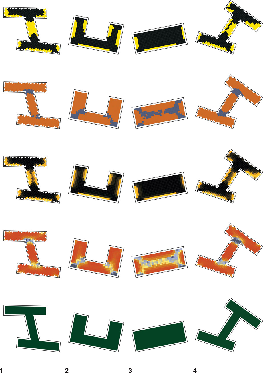
Figure 7.15 Small office mixed shapes for Miami at 1:100 (approximate).

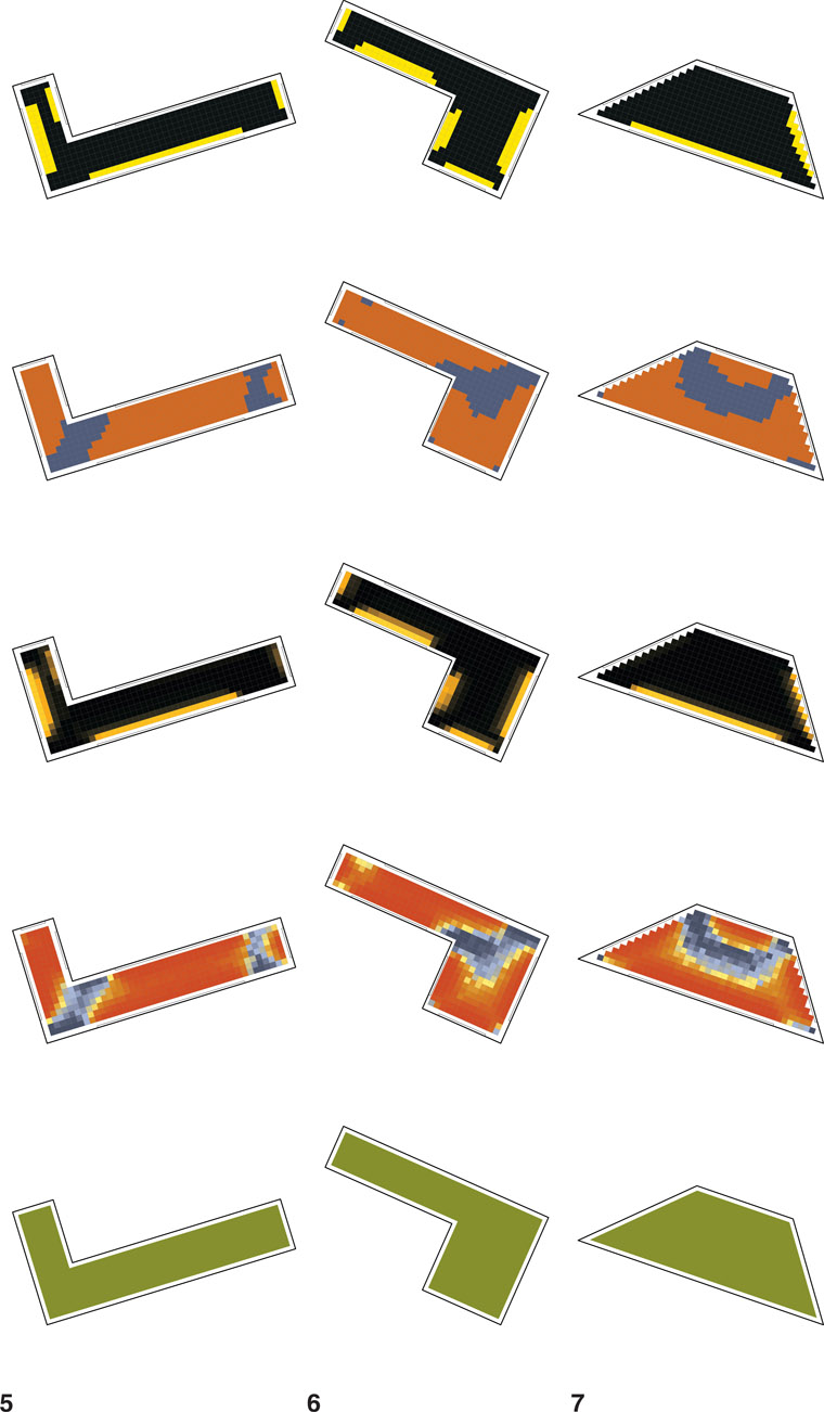
Figure 7.16 Small office mixed shapes for Miami at 1:100 (approximate).

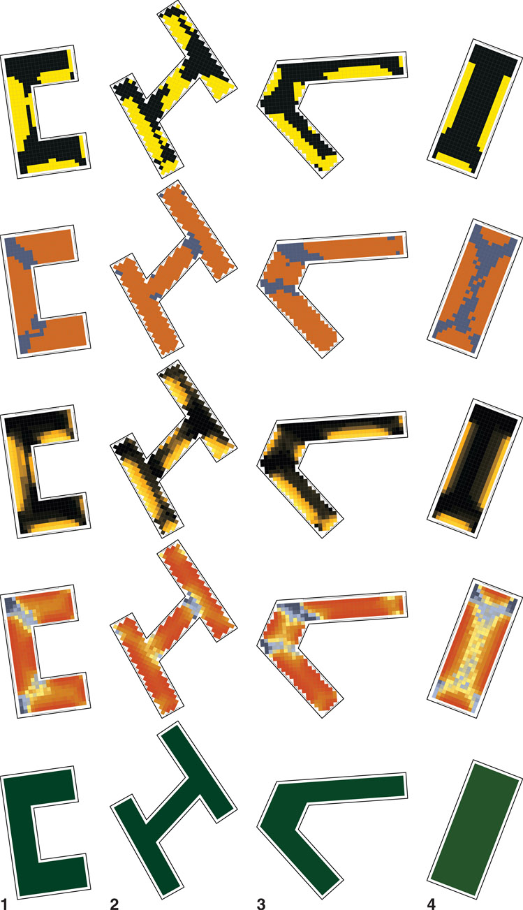
Figure 7.17 Small office mixed shapes for New York at 1:100 (approximate).

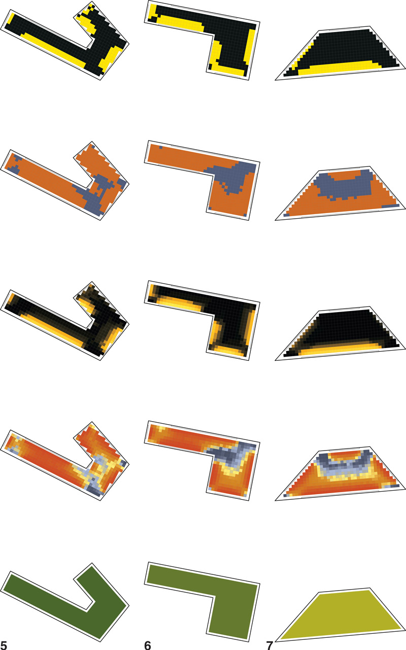
Figure 7.18 Small office mixed shapes for New York at 1:100 (approximate).

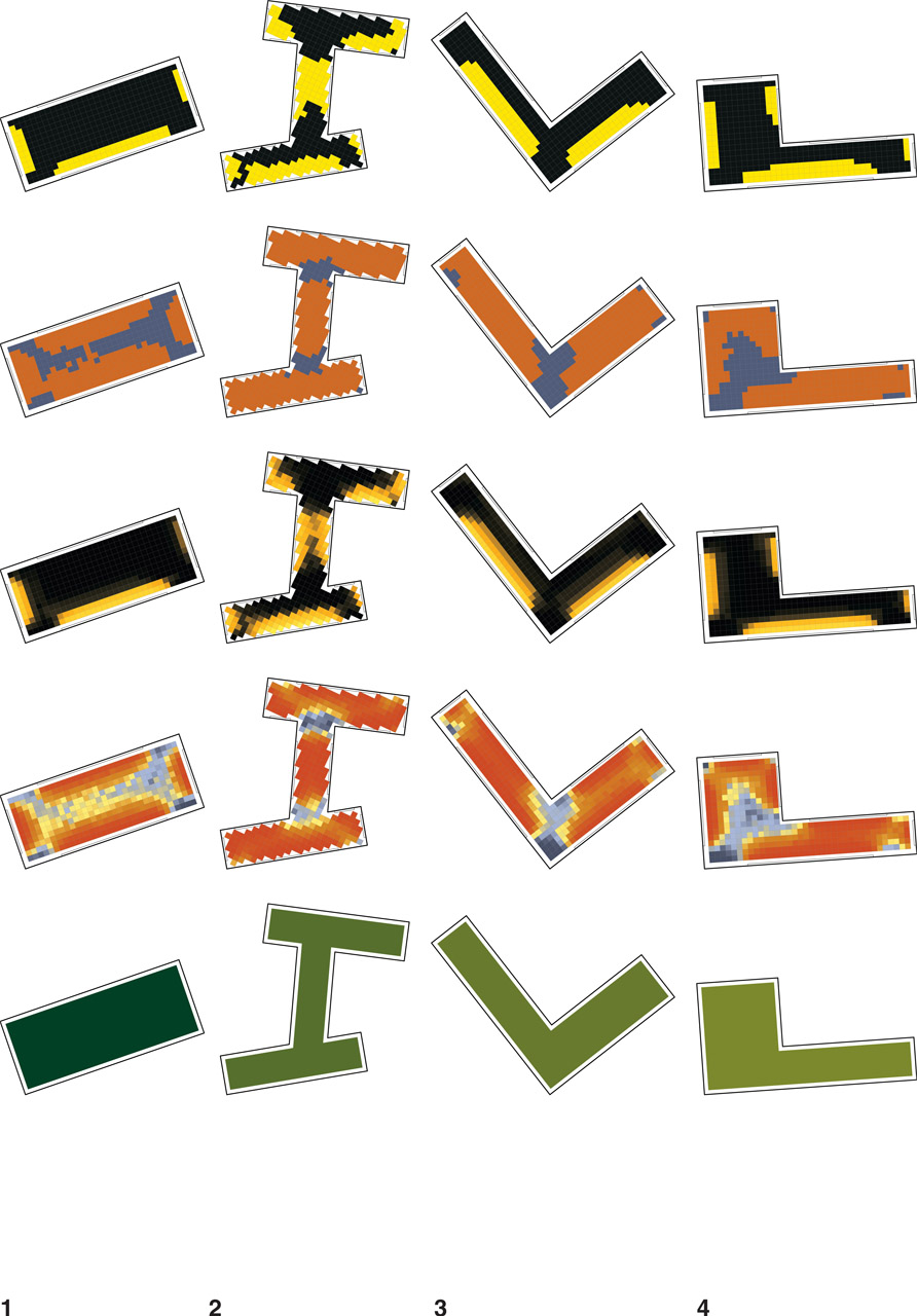
Figure 7.19 Small office mixed shapes for Omaha at 1:100 (approximate).

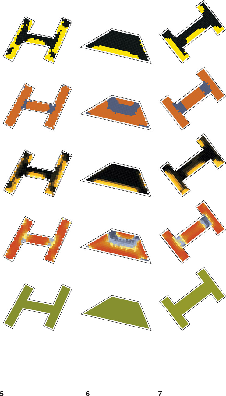
Figure 7.20 Small office mixed shapes for Omaha at 1:100 (approximate).

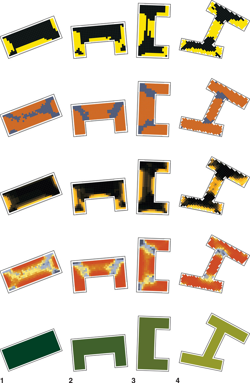
Figure 7.21 Small office mixed shapes for Phoenix at 1:100 (approximate).

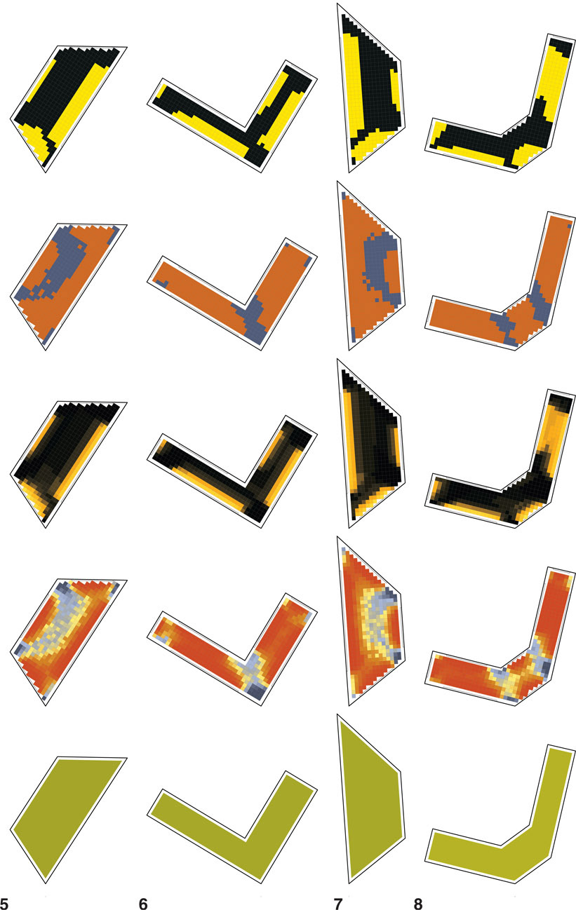
Figure 7.22 Small office mixed shapes for Phoenix at 1:100 (approximate).

Figure 7.23 Medium office mixed shapes for Miami at 1:300 (approximate).

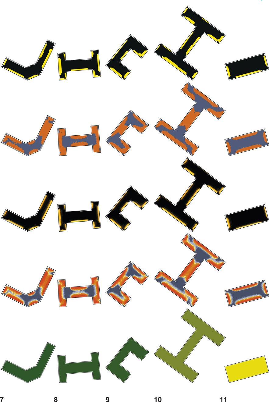
Figure 7.24 Medium office mixed shapes for Miami at 1:300 (approximate).

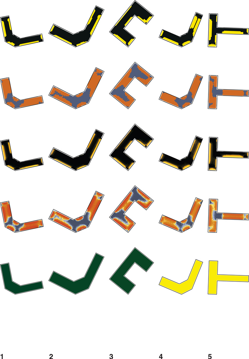
Figure 7.25 Medium office mixed shapes for New York at 1:300 (approximate).

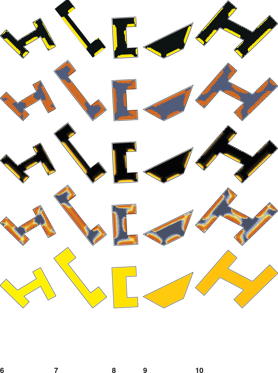
Figure 7.26 Medium office mixed shapes for New York at 1:300 (approximate).

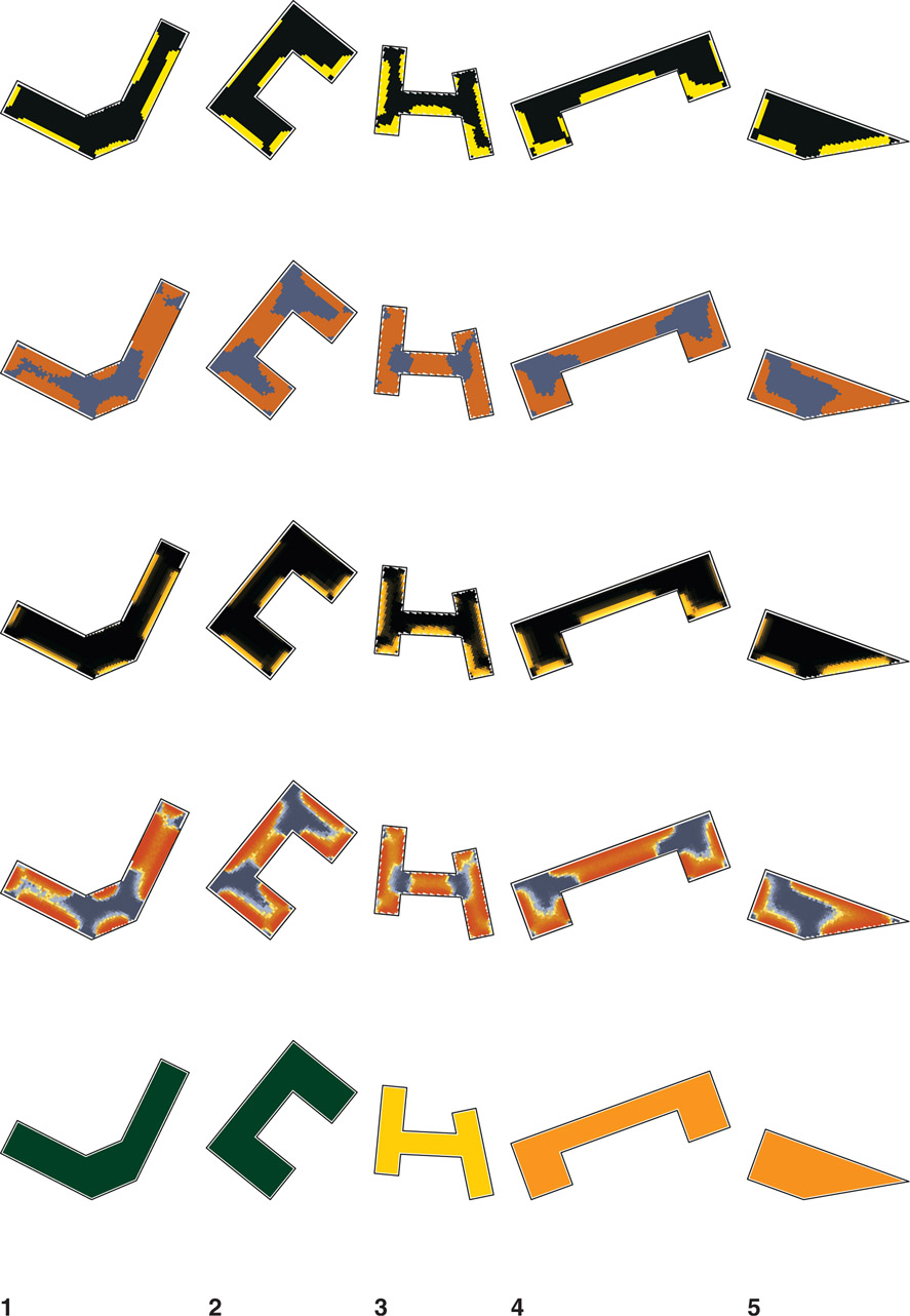
Figure 7.27 Medium office mixed shapes for Omaha at 1:300 (approximate).

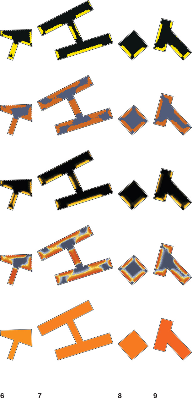
Figure 7.28 Medium office mixed shapes for Omaha at 1:300 (approximate).

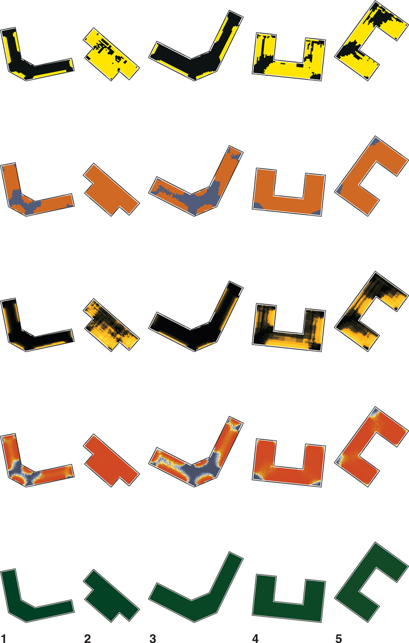
Figure 7.29 Medium office mixed shapes for Phoenix at 1:300 (approximate).

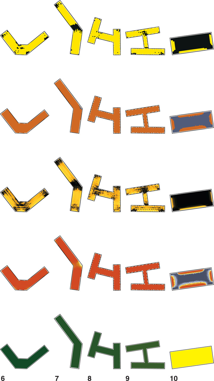
Figure 7.30 Medium office mixed shapes for Phoenix at 1:300 (approximate).

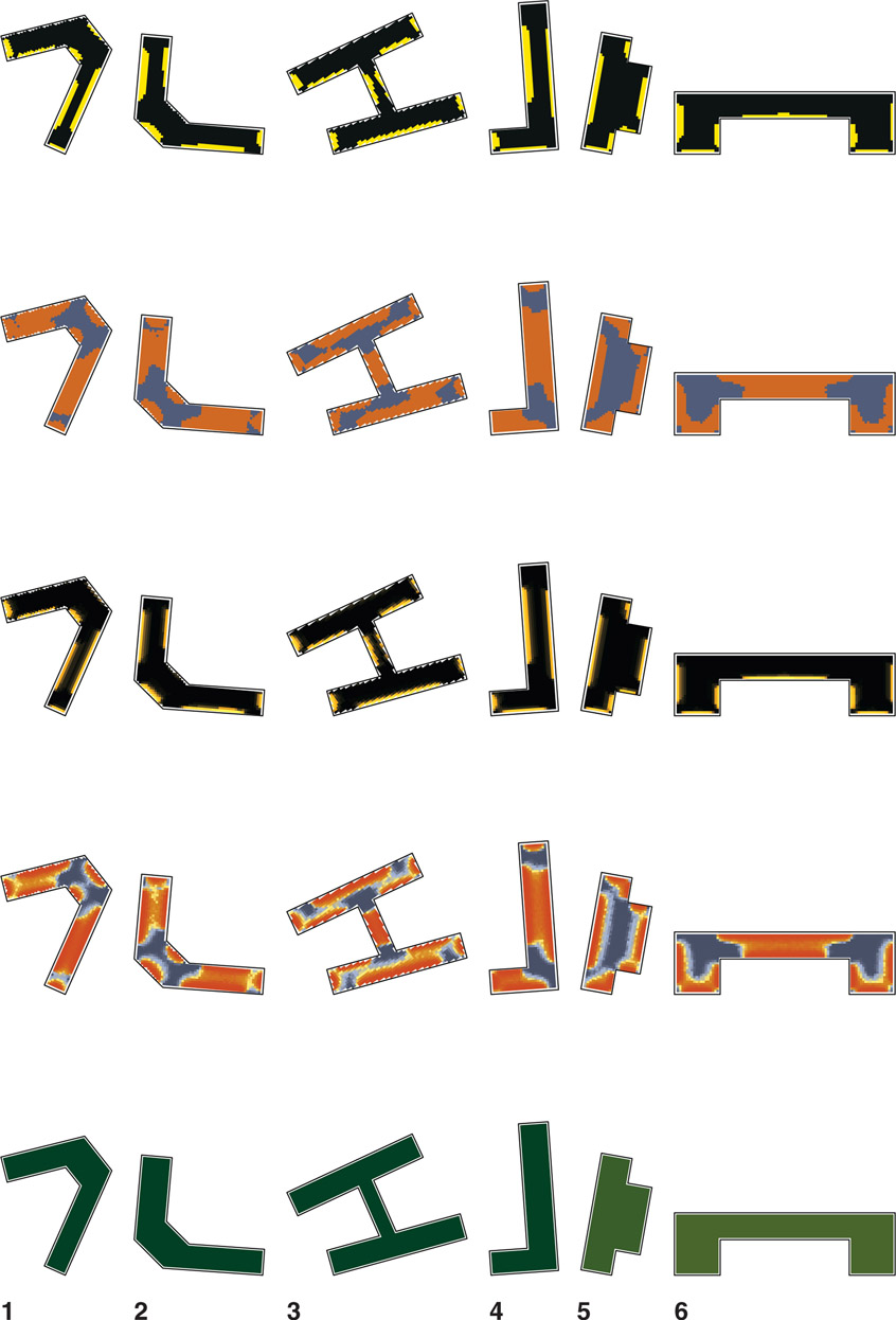
Figure 7.31 Large office mixed shapes for Miami at 1:500 (approximate).

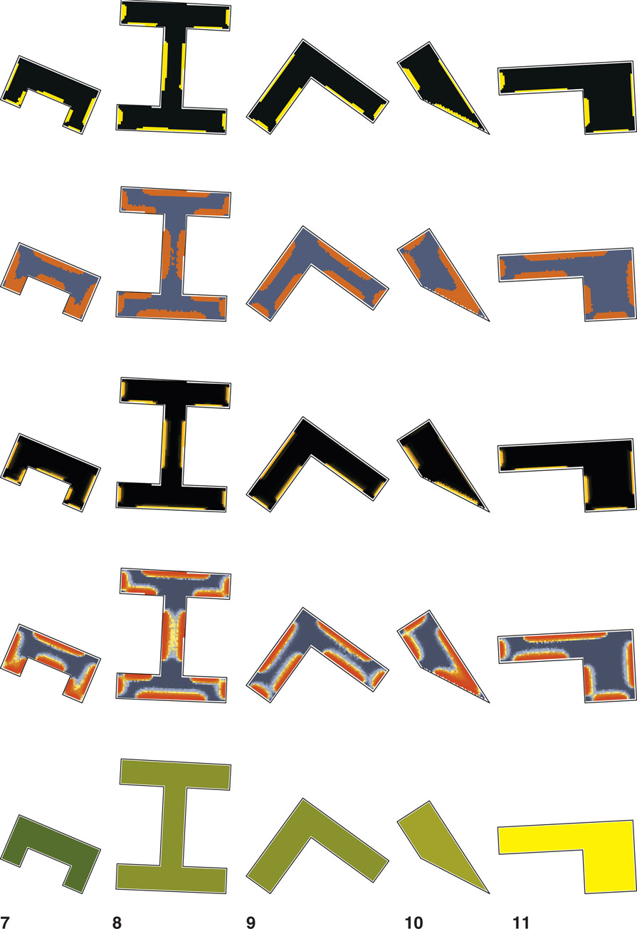
Figure 7.32 Large office mixed shapes for Miami at 1:500 (approximate).

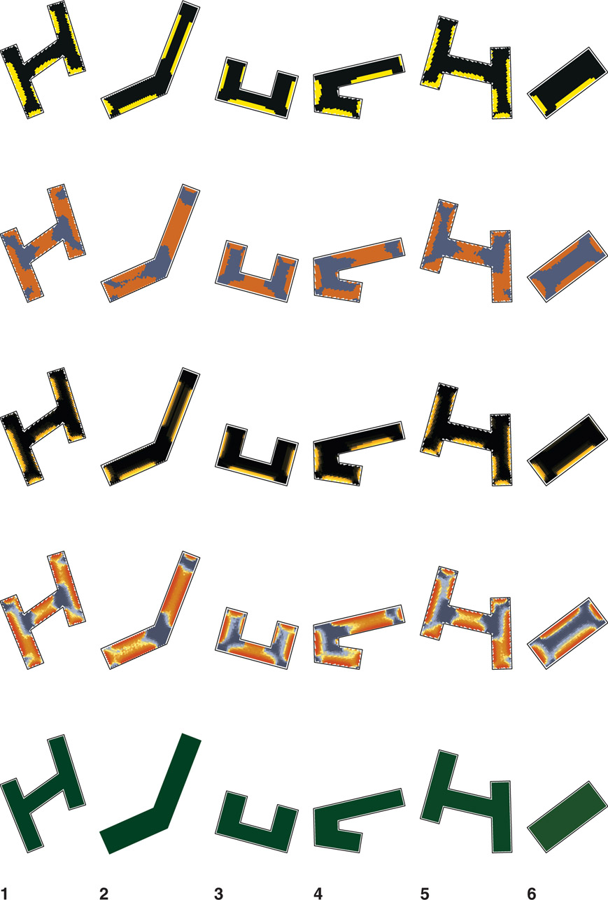
Figure 7.33 Large office mixed shapes for New York at 1:500 (approximate).

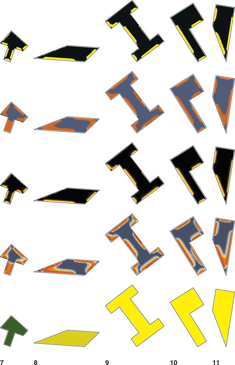
Figure 7.34 Large office mixed shapes for New York at 1:500 (approximate).

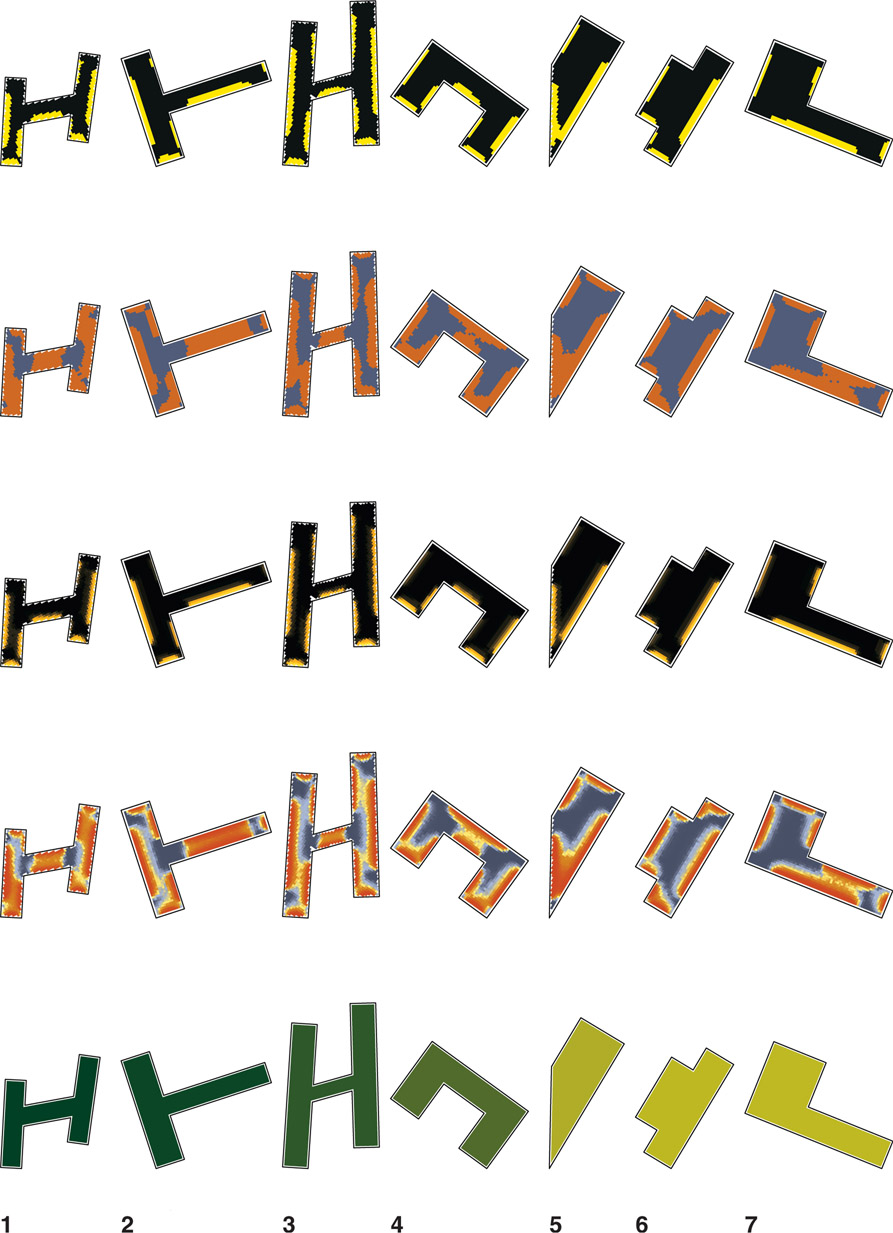
Figure 7.35 Large office mixed shapes for Omaha at 1:500 (approximate).

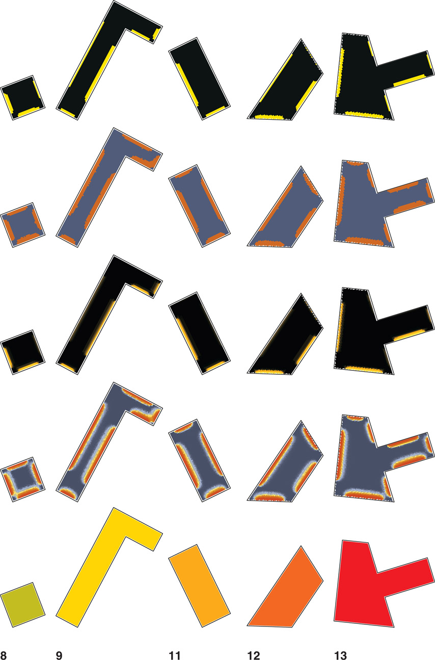
Figure 7.36 Large office mixed shapes for Omaha at 1:500 (approximate).

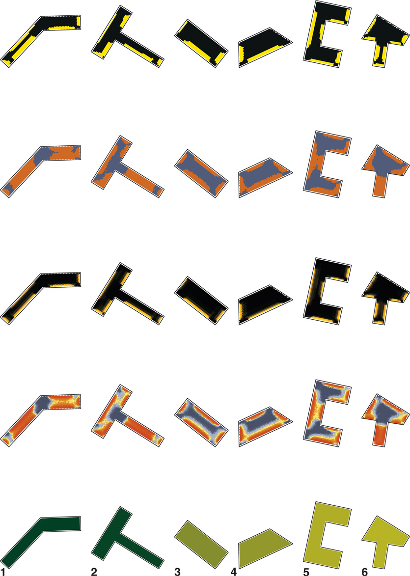
Figure 7.37 Large office mixed shapes for Phoenix at 1:500 (approximate).

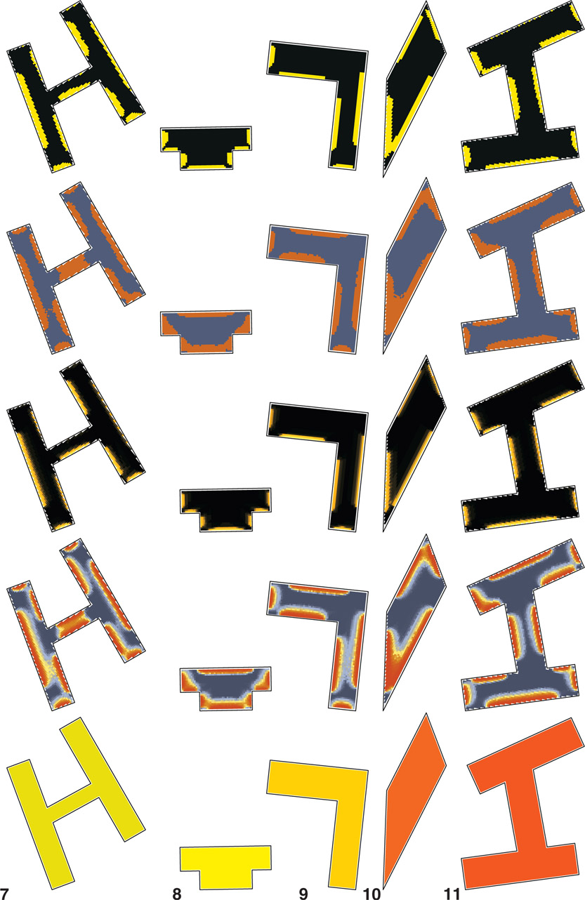
Figure 7.38 Large office mixed shapes for Phoenix at 1:500 (approximate).

Examples of whole-building models

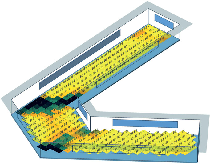
Figure 7.39 Axonometric view of a small U-shaped office in New York.

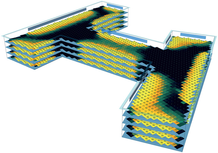
Figure 7.40 Axonometric view of a medium H-shaped office in New York.

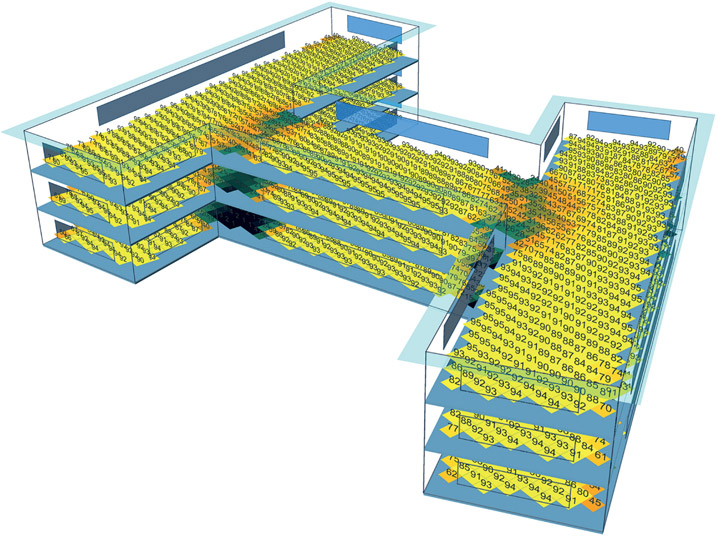
Figure 7.41 Axonometric view of a medium H-shaped office in New York.

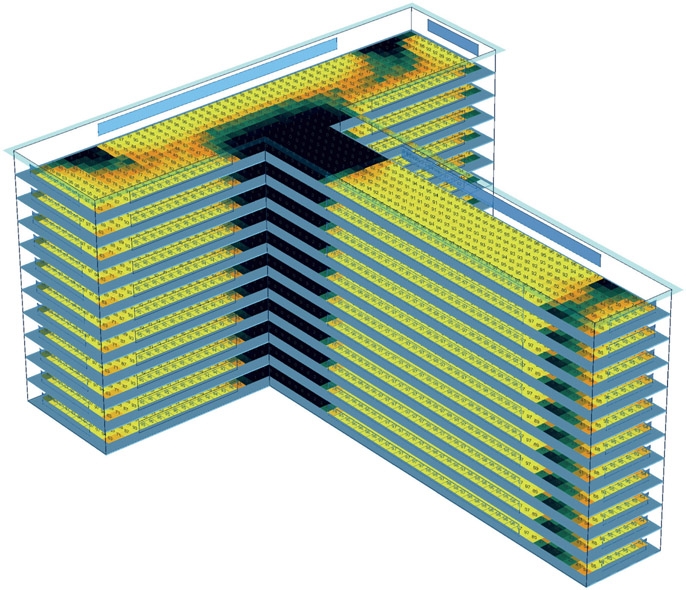
Figure 7.42 Axonometric view of a large T-shaped office in Miami.

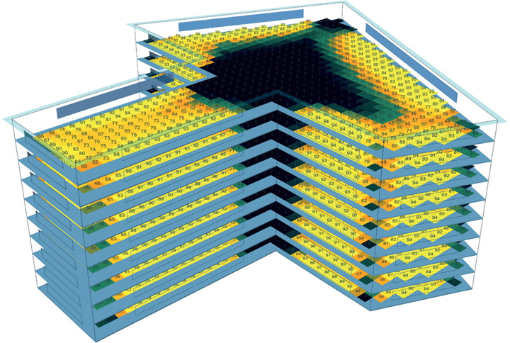
Figure 7.43 Axonometric view of a large T-shaped office in Omaha.

The End?

Not so fast. Our argument is that the energy performance and daylighting presented in the pattern guide are difficult to predict without the aid of simulation. The results of the pattern guide show how closely similar shapes may lead to very different results. Therefore, first the point is that it is hard to predict these tendencies with rules of thumb for daylighting (effective daylight depth is two times the height of the window). Second, linking daylighting and energy in one simulation result provides a more honest picture of the whole building’s performance. This is what simulation is about: Providing more information than we had to begin with in order to make the best decision, whether we are using the BEM to understand, to compare, or to forecast the energy performance of our design decisions.

Daniel Overby discusses this on his blog with a post titled, “Every Energy Model is Wrong—And Here is Why They are Indispensable,”¹⁴ and highlights that BEM is beneficial because now there is more information than before. Our process of discovery in this chapter highlights the deficiency of the existing BEM simulation methodologies. This entire book highlights our own research and explorations; therefore, the appropriate conclusion is that there is still much to learn, much to come in the future, and much more to explore using building energy and parametric modeling, scripting, and algorithms. This entire process comes in the pursuit of a new kind of built environment—that is, a carbon-neutral one.

Notes

1 Bernard Tschumi et al., “Introduction,” in Tschumi Le Fresnoy: Architecture In/ Between (New York, NY: The Monacelli Press, 1999), 9.

2 IES Daylight Metrics Committee, Approved Method: IES Spatial Daylight Autonomy (sDA) and Annual Sunlight Exposure (ASE), IES. LM-83-12 (New York, NY: IES, 2012), 2.

3 Kyle Konis, Alejandro Gamas, and Karen Kensek, “Passive Performance and Building Form: An Optimization Framework for Early-Stage Design Support,” Solar Energy 125 (2016): 161–179.

4 Ibid., 165.

5 Ibid., 173.

6 “performLive,” http://performlive.com/design_brief.pdf.

7 RapidTables.com “Lux to watts calculator,” www.rapidtables.com/calc/light/lux-to-watt-calculator.htm.

8 IES, Approved Method, 3.

9 Ibid., 4.

10 Since the study is executed in DIVA, the materials and compositions are also extracted from DIVA sources.

11 IES, Approved Method, 3.

12 Ibid.

13 To keep the results consistent, the technical report M. Deru and P. Torcellini, Source Energy and Emission Factors for Energy Use in Buildings, NREL/TP-550-38617 (Golden, CO: NREL, 2007) is used, which is also DIVA’s source.

14 Daniel Overbey, “Every Energy Model is Wrong—And Here is Why They are Indispensable,” August 5, 2016, http://danieloverbey.blogspot.com/2014/08/every-energy-model-is-wrong-and-here-is.html.