The operators that can be used in Excel formulas span the entire range of commonly used symbols. These operators are listed in this section, with the most frequently used described first.
Arithmetic operators are used for basic calculations and return numeric values. Table 3-1 lists the arithmetic operators used in Excel formulas.
You create formulas in Excel worksheets by using these operators and entering the formulas directly into a cell. After you enter a formula, the result is displayed in the cell and the formula is shown as the cell content in the formula bar.
To change the priority of calculation operations, put the expressions you want to calculate first in parentheses. Enter both formulas shown in Table 3-2 in different cells and compare the results to test the functionality of parentheses.
Note
In a formula, the number of opening parentheses must match the number of closing parentheses. Otherwise, Excel reports an error and highlights the incorrect part of the formula or offers to correct the formula.
Excel provides input assistance to ensure that you don’t lose track of the parentheses and to verify that the number of opening parentheses matches the number of closing parentheses:
If you enter a closing parenthesis, the opening parenthesis is highlighted for a few seconds in the formula bar or in the cell.
If you edit an existing formula and point to one of the parentheses, the matching parentheses are highlighted for a few seconds (depending on your settings).
If an expression contains several operators, the priority for calculation is determined by the priority of the operators. You can change the standard priority by using parentheses within a formula. Table 3-3 shows the priority for the operators within an Excel formula.
Table 3-3. Operator Priority
Priority | Operator | Description |
|---|---|---|
1 | – | Negation of a value (for example, –34) |
2 | % | Division of a value by 100 (percent) |
3 | ^ | Exponentiation of a value |
4 | * and / | Multiplication and division |
5 | + and – | Addition and subtraction |
You might remember the old arithmetic rule, PEMDAS, which can help you when you are in doubt.
Use the comparison operators to compare values, text, or cells. These expressions are often used in logical functions; a common example is IF(). The result is always a logical value (Boolean value). Table 3-4 lists all of the Boolean operators and illustrates them with sample formulas.
In some cases, you might want to combine the results from several formulas or cells in a single cell. For this task you use the & (ampersand) operator. If you connect two values of any type with the ampersand, the result always has the Text data type. In other words, Excel converts number values automatically into text. This way you can use the text operator to include two number values as text in one cell. However, you cannot use the resulting string directly for other calculations.
Note
If you use text instead of a cell reference in a formula, you must put this text in quotation marks. You don’t have to put numbers in quotation marks. Quotation marks are also not necessary if you use references to cells, which can contain any data type.
To connect the content in cells A1 and A2 by using the text operator, use the following formula:
=A1&A2
The text operator connects the contents of the two cells without a space in between them. To include a space between the values, you must use quotation marks. If you want a space between the values in cell A1 and cell A2, use the following formula:
=A1&" "&A2
Sample Files
Use the Text Operator worksheet in the Chapter03.xls or Chapter03.xlsx sample file. The sample files are found in the Chapter03 folder. For more information about the sample files, see the section Using the Sample Files. Figure 3-2 shows the content of this worksheet.

With reference operators, you can pass cells or cell ranges to a formula or function for calculation. The following operators are available:
Range separator : (colon). Creates a reference to all cells between two references, including the reference cells themselves; for example—B3:B20
Connection operator , (comma). Allows the connection of several cells or references in an expression—for example, SUM(B3:B20,D3:D20)
Intersection operator (space). Creates a reference to cells that occur in both ranges that are referenced; in other words, the cells are the intersection of both ranges—for example, B7:D7 C6:C8
A range is an area of a worksheet consisting of cells next to and/or below each other. If two cell references are connected with a colon, these references together with the cells in between form a range. Ranges can have different sizes and shapes. In functions, a range is an argument independent of its size.
Possible Range References. Range references are easily specified. Figure 3-3 shows all of the possible variations.
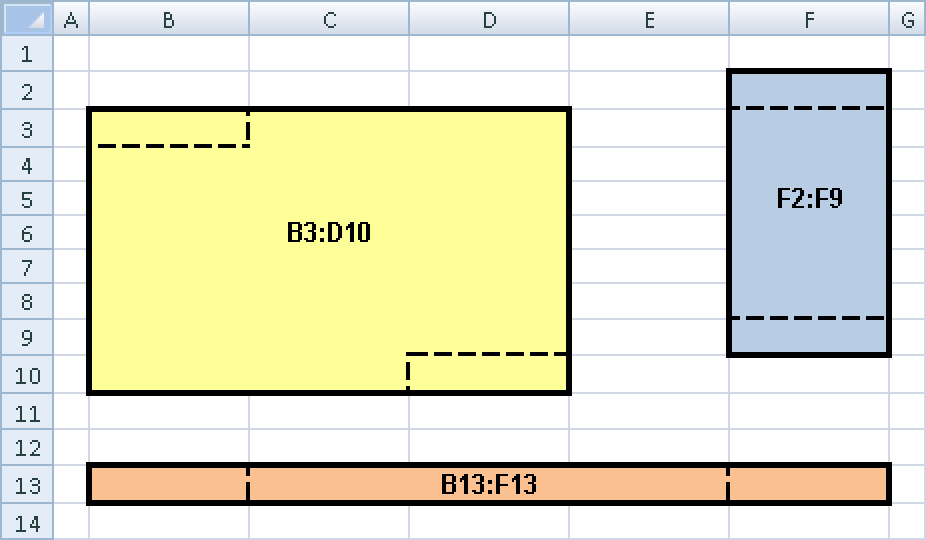
The ranges shown demonstrate the following rules for range reference syntax:
For a range spanning several columns and rows, the cell in the upper-left corner is connected with the cell in the lower-right corner, as in B3:D10.
For a range spanning one row, the left cell is linked with the right cell, as in B13:F13.
For a range spanning one column, the upper cell is linked with the lower cell, as in F2:F9.
If you want to reference columns or rows from the first to the last cell, use the references listed in Table 3-5. You can create references for other columns and rows based on the references in this table.
You can pass nonadjacent cells to a function for calculation by using a connection, or union, operator. The connection operator is the comma (,). If you use the connection operator to pass several cells to a function, each cell reference that is separated from another by a comma is treated as a separate argument.
If you wanted to add the three ranges shown earlier in Figure 3-3, you would have to specify each cell group in the SUM() function. The function would have three arguments separated by commas:
=SUM(B3:D10,F2:F9,B13:F13)
The intersection operator is rarely used but should be included on this list. With the intersection operator (the space), you define a reference to the cells shared by several different references. In other words, an intersection in Excel describes the values in the area where two or more ranges overlap.
The intersection shown in Figure 3-4 is where the ranges B2:E11 and C8:G14 overlap. In a formula or function, this intersection would look like this: B2:E11 C8:G14.
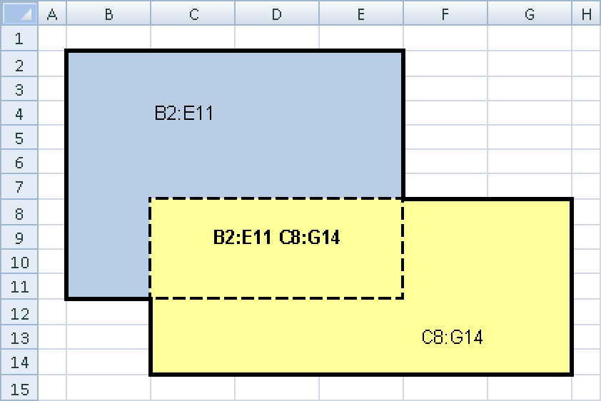
The result of the intersection is called an explicit intersection. The values in the cells in the explicit intersection are added up with the following formula:
=SUM(B2:E11 C8:G14)
Intersections are mostly used in the context of range names and are rarely used as pure cell references.