In this section, you see some tips and tricks you can use when working with formulas. Depending on how often you use Excel, you might find some of the following procedures more useful than others.
To get an overview of a sheet with many formulas and connections, you can view the underlying formulas instead of the results. This is often useful if the sheet was created by someone else:
Open the worksheet.
Press Ctrl+` (the key to the left of the number 1 on the keyboard).
Excel switches from displaying the results to displaying the underlying formulas. Because the formulas need more space, Excel adjusts the column width automatically.
Note
The Ctrl+` key combination doesn’t change the data in your table. This command only affects the view; you can reset by pressing Ctrl+` again.
You can also switch to the formula view by clicking the Show Formulas button on the Formula tab in the Formula Auditing group. You can also make this change in the Excel Options dialog box. Figure 3-16 shows the Show Formulas In Cells Instead Of Their Calculated Results check box in the Advanced section of the Excel 2010 Options dialog box.
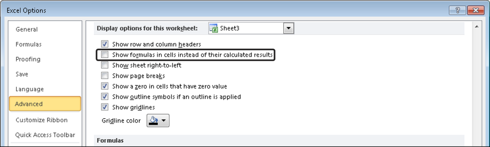
In all Excel versions, these settings apply only to the active worksheet.
If you know that a formula has to be entered into several cells, you can enter the formula in three simple steps:
Click the cell in which you want to enter the formula and extend the selection to the range that will contain the copied formula. A multiple selection is also possible.
Enter the formula in the active cell.
Press Ctrl+Enter after you enter the formula.
The selected range is filled with the formula.
In workbooks with similar sheets, you can enter formulas (or other content) in several worksheets at the same time. You just have to select (group) the desired sheets:
Hold down the Ctrl key and select the sheet tabs of the sheets you want to group. Group mode is indicated in the title bar of the window.
Enter the formula (or formulas) in the active sheet.
To ungroup, select a sheet or use the Ungroup command to ungroup all the sheets, right-click a selected sheet tab to display a shortcut menu.
The formula (or formulas) are written in all selected sheets. You can also combine the method shown previously for entering formulas in several rows with the method for entering formulas in several sheets.
Excel highlights all cells containing formulas if you perform the following steps:
If you have to work through all selected formula cells, press the Tab key to switch between the selected cells. You can also edit a formula in the formula bar. Press Shift+Tab to move in the opposite direction.
To unselect but still work through all formulas, assign a color to the selected cells (you can remove the color later).
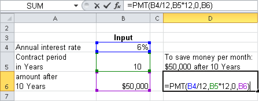
To see which cells a formula refers to, press the F2 key. This opens the cell for editing and shows the cell references in different colors (see Figure 3-17).
In large tables, entering each formula requires a lot of effort. If you know how to copy formulas you can reduce the amount of work required to enter formulas. The same applies to corrections. If you know how to move formulas and values, you can quickly rearrange your table.
You must always select the range you want to copy or move. As with all Windows applications, you have two options for making a selection:
You can use the keyboard or a command.
You can use the mouse.
The most comfortable way to make a selection is by using the mouse. However, sometimes it makes sense to make a selection by pressing a key combination. Table 3-6 lists several key combinations you can press to make a selection.
Table 3-6. Making a Selection by Using the Keyboard
Selection | Key Combination |
|---|---|
Current row | Shift+Spacebar |
Current column | Ctrl+Spacebar |
Current data block | Ctrl+Shift+* |
From the current cell in any direction | Shift+arrow key |
From the current cell to the end of the data block | Shift+Ctrl+End |
From the current cell to the beginning of the data block | Shift+Ctrl+Home |
Entire sheet | Ctrl+Shift+Spacebar or Ctrl+A |
To extend the selection beginning at the current cell, press the F8 key. Excel switches into “extension mode,” as indicated by EXT (in Excel 2003) or Extend Selection (in Excel 2010) in the status bar. In this mode, you can use the arrow keys to extend the selection in any direction. To disable extension mode, press F8 again or press the Esc key.
To select a cell range, drag over the range you want to select. Table 3-7 lists useful approaches for making a selection with the mouse.
Table 3-7. Making a Selection by Using the Mouse
Selection | Action |
|---|---|
A single cell | Click in the cell. |
A column | Click the column heading. |
Several columns | Drag over the column headings. |
A row | Click the row heading. |
Several rows | Drag over the row headings. |
A connected cell range | Drag diagonally from the first to the last cell. |
Unconnected cells or noncontiguous cell ranges | Hold down the Ctrl key and click additional cells or cell ranges, columns, or rows. |
All cells in the worksheet | Click the button in the upper-left corner of the worksheet window. |
You have to select the entire table to make a global change (for example, to change the font).
To move a formula cell, you actually delete the formula in the original cell and paste it into another cell. There are two approaches to do this:
In Excel 2003, select the Cut and Paste options on the Edit menu or click the corresponding buttons on the toolbar. In Excel 2007 and Excel 2010, click the buttons in the Clipboard group on the Home tab.
Move a formula by using the mouse.
To move a formula cell to another location within a table, perform the following steps:
Click the Cut button in the Clipboard group on the Home tab or press Ctrl+X.
Select the target cell. If you move a cell range, the target cell is the upper-left cell of the new range.
Click the Paste button in the Clipboard group on the Home tab or press Ctrl+V.
After you have moved the cell, check whether the formula or the result has changed. The result is displayed in the table and should match the previous result. To review the formula, click the cell you moved and check the formula bar. The cell content as well as the formula stay the same if a cell is moved.
If you don’t want to use the Clipboard, you can move a formula cell by using the mouse. With the mouse, you can move cells easily to another location within the table. Do the following:
Select the cell or cells you want to move.
Move the mouse pointer to the border of the selection. The pointer changes to a white arrow with a black double arrow (see Figure 3-18).
Drag the cell or cells to the new location.
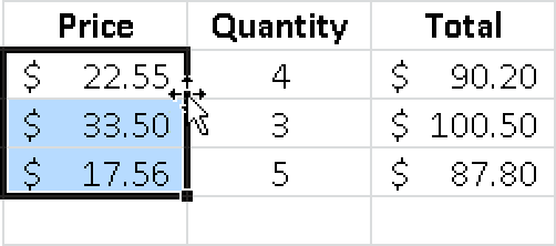
While being dragged, the moved range is highlighted in gray. Next to the highlighted range, a tooltip shows the cell reference or the cell range to which the highlighted range will be moved when you release the mouse button.
If you move the cells into a range already containing data or formulas, Excel asks if you want to overwrite the content of the target range. This ensures that no data will be lost if cells are moved accidentally.
If you copy data, the data remains in the initial location and a copy of the data is pasted at another location. When copying formulas, it is important to know whether the formula references are relative, absolute, or mixed (see the section References in Formulas earlier in this chapter).
The following approaches are available for copying formulas:
Selecting the Copy and Paste options in the Clipboard group on the Home tab
Copying the formula cell by using the mouse
Dragging the fill handle of the formula cell
The results of the first two approaches are the same.
To copy by using the a key combination or the buttons on the Home tab, perform the next set of steps:
Select the cell or cells you want to copy.
Click the Copy button in the Clipboard group on the Home tab, or press Ctrl+C.
Select the target cell or cells. If you copy a cell range, the target cell is the upper-left cell of the range.
Click the Paste button in the Clipboard group on the Home tab, or press Ctrl+V.
Note
To paste the copied cells again, repeat step 4. This also applies to pasting by using the Cut command in the Clipboard group on the Home tab.
If you press Enter to finish the move or copy operation, Excel deletes the content of the Clipboard, and the data cannot be moved or copied again from the Clipboard.
To copy cells by using the mouse, you basically do the same as you would to move cells with the mouse. Perform the following steps:
Select the cell or cells you want to copy.
Move the mouse pointer to the border of the selection. The pointer changes to a white arrow with a black double arrow.
Press the Ctrl key. The double arrow is replaced by a plus sign (see Figure 3-19).
Holding down the Ctrl key, drag the cell or cells to the new location. Release the mouse button and then the Ctrl key.

Make sure you release the mouse button first and then the Ctrl key. If you release the Ctrl key first, the copy command is canceled and the cell content is moved.
Click the copied cells and review the cell content in the formula bar to check whether the content has changed. For a better understanding, see the next section.
In Figure 3-20, the formula in cell D4 was copied to several different locations. Remembering the section Relative References earlier in this chapter, ask yourself the following questions: What calculation is related to the original cell (cell D4 in Figure 3-20)? Which cells, starting at cell D4, should be multiplied? What does the calculation look like after the cells are copied?
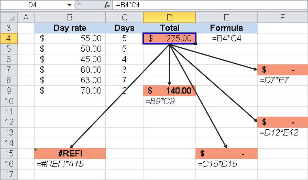
The calculation in cell D4 could read like this: “Multiply the two adjacent cells on the left.” This calculation was copied exactly to all other cells:
In cells E15, F7, and F12, the result is 0 because the two adjacent cells on the left are empty.
In cell B15, the first cell reference generates the error message #REF!, which is returned by the formula as the final value. The referenced cell B4 cannot be transformed when you copy the formula two columns to the left.
Only the result in cell D9 makes sense, because the two adjacent cells contain values that can be multiplied.
In other words: The cell references changed in relation to their locations, but the initial calculation—embedded in the formula—remains the same at all locations.
As you already know, a cell reference with these properties is called a relative reference. If you want the copied formulas to anchor on particular cells, you have to use absolute or mixed cell references.
The Fill function in Excel offers several possibilities for copying formulas quickly and accurately.
The Fill Menu Command in Excel 2003. The Edit/Fill menu command achieves good results. Do the following:
Click the cell containing the formula you want to copy, and extend the selection in any direction (down, up, right, or left).
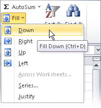
In Excel 2003, select the Edit/Fill menu option and select a fill direction. In the case shown in Figure 3-21, you would have to select Down.

In Excel 2007 and Excel 2010, only a few clicks are necessary to select the fill direction: Select the direction on the Fill list in the Edit group on the Home tab (see Figure 3-22).
Using the mouse is probably the easiest and most commonly used approach for filling cells. In the lower-right corner of the active cell or of a selected range is the fill handle. If you point to the fill handle, the mouse pointer changes into a black plus sign. Drag the fill handle over the range into which you want to copy the formula.
If you drag over the cell (or cells) containing the formula, the cell is highlighted in gray. If you release the mouse button at this point, the content of the gray cell is deleted. If this happens, click the Undo button on the toolbar or in the Quick Access Toolbar (Excel 2007 and Excel 2010), or press Ctrl+Z.
The smartest way to fill cells is to double-click. However, this approach has the following restrictions:
Cells can be filled only from the top down.
The fill range follows the data in the column to the left and fills down as far as data is displayed. (Note, however, that if columns are hidden, the fill range will follow the data in the column that is visible to the left of the fill range.)
Any existing data or formulas in the fill range may be overwritten without warning.
To fill adjacent cells with a double-click, perform the following steps:
Select the cell that contains the formula you want to copy.
Point to the fill handle until the mouse pointer changes into a plus sign.
Double-click to fill the range with the formula.
There are many occasions when you may want to fix your data. For example, you might need to archive a snapshot of the results and want to avoid recalculation, or you might want to avoid having data linked back to other workbooks.
To convert results to fixed values, you use the right mouse button:
Select the cells containing formulas or connections.
Right-click the border of the selected cells and drag the selection one column to the right and then back again.
On the shortcut menu, select Copy Here As Values Only.
Or use the Copy and Paste functions:
Select the cells containing formulas or connections.
Select the Edit/Copy option or press Ctrl+C.
Select the Edit/Paste Special option (Excel 2003) or Paste/Paste Special in the Clipboard group on the Home tab (Excel 2007 and Excel 2010).
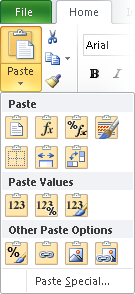
Select the Values option in the Paste Special dialog box and click OK. Alternatively, you can select Values (Excel 2003) or Paste Values (Excel 2007 and Excel 2010) on the Paste list on the toolbar. Excel 2010 provides more options for pasting values (see Figure 3-23).
Assume that you have a table of readings in meters that you want to convert to feet. Follow these steps:
Enter the conversion factor 3.2808399 into any cell, and press the Enter key.
Select the cell containing the conversion factor.
Press Ctrl+C.
Select the range containing the readings in meters.
Select the Edit/Paste Special option (Excel 2003) or Paste Special on the Paste list (Excel 2007 and Excel 2010).
Select the Divide option, and click OK.
To prevent your formulas from being changed by other users, you can protect certain cell ranges or formula cells.
There are two points to remember when protecting cells. First, all cells are locked by default. Second, the lock is activated only when the sheet is protected. Common practice is to leave all cells protected and unlock only those in which you want users to enter information.
To do this, perform the following steps:
Select the cell range in which you will allow users to enter information.
Right-click the selected range, and select the Format Cells option.
Click the Protection tab, and clear the Locked check box. Click OK.
On the Tools menu, select Protection/Protect Sheet (Excel 2003), or click the Protect Sheet icon on the Review tab (Excel 2007 and Excel 2010).
Create a password if you want to add a further layer of protection.
Click OK to activate the sheet protection.
Now other users cannot enter information into any cells other than those that have been unlocked.
If you want to protect only a limited number of cells, start by selecting the entire sheet and unlocking the cells by using the Format Cells option. Then repeat the preceding steps to lock a selection of cells. Finally, protect the sheet.
You can go one step further and ensure that the formulas in your formula cells are not displayed in the formula bar. To do this, perform the following steps:
Select the cell range containing the formulas you want to protect.
Right-click the selected range, and select the Format Cells option.
Select the Hide check box on the Protection tab, and click OK.
On the Tools menu, select Protection/Protect Sheet (Excel 2003), or click the Protect Sheet icon on the Review tab (Excel 2007 and Excel 2010).
Create a password if you want to add further protection.
Click OK to activate the sheet protection.
Regardless of whether the cell is locked, the formula is not displayed in the formula bar when the sheet is protected.
You can specify when Excel should perform a calculation. You can find the options for this in Tools/Options on the Calculation tab (Excel 2003). In Excel 2007 and Excel 2010, use the buttons in the Calculation group on the Formulas tab (see Figure 3-24).

Figure 3-24. The three icons in the Calculation group on the Formulas tab of Excel 2007 and Excel 2010.
The following options are available:
Automatic. Calculates all dependent formulas if a value, a formula, or a name changes. This is the default setting.
Automatic Except For Data Tables. Calculates all dependent formulas except data tables. To calculate data tables, click the Calculate Now button on the Formulas tab or press the F9 key.
Manual. Only calculates open workbooks if you press the F9 key or click the Calculate Now button on the Formulas tab. If you select Manual, Excel automatically activates the option to recalculate the workbook before saving.
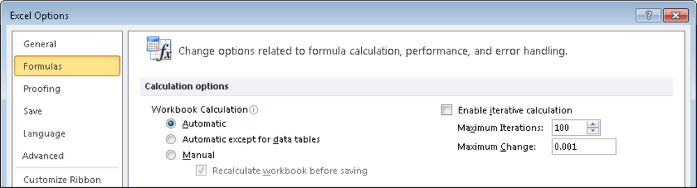
All settings are available on the File tab, by choosing Options and clicking the Formulas tab. Figure 3-25 shows the calculation options in Excel 2007 and Excel 2010, which reduced the selection available from previous versions.
When you edit a formula, Edit mode shows all of the cells and cell ranges referenced in the formula, as well as their borders, in specific colors. This way you can easily create cell references.
To switch into Edit mode, double-click the formula cell or select the formula cell and press the F2 key.
You can use formula auditing to show the relationships between cells. To check which cells are used by a formula, enable formula auditing.
Until Excel 2007, this command was on the Tools menu and was called Formula Auditing. The descriptions in this book are for Excel 2002, Excel 2003, Excel 2007, and Excel 2010.
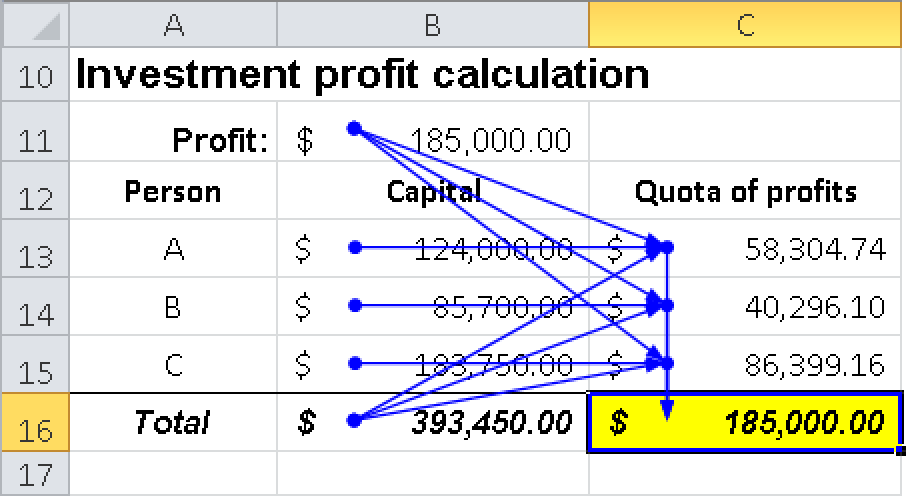
Formula auditing reduces the task to a few mouse clicks and shows the result (see Figure 3-26). Select the relevant formula cell and then the Tools/Formula Auditing/Trace Precedents option.
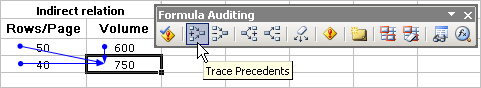
Tracer arrows show the flow of values and formula results in a worksheet. This allows you to find and view precedents (cells referenced in a formula) and dependents (cells with references to other cells).
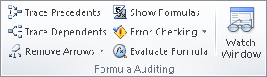
The Formula Auditing toolbar in Excel 2003 (shown in Figure 3-26) was replaced with the Formula Auditing group on the Formulas tab in Excel 2007 and Excel 2010 (see Figure 3-27).
Assume that you want to find out which cells or cell results are included in the formula in a certain cell. The formula audit allows you to trace the flow of formulas and data. To do this, perform the following steps:
Select the start cell for the audit. This cell can include a formula, or a formula might refer to the cell or contain an error message.
In Excel 2003, select Formula Auditing from the Tools menu. In Excel 2007 and Excel 2010, select the Formulas tab to access the Formula Auditing options (shown earlier in Figure 3-27). The following options are available:
Trace Precedents. The first time you select this option, you see traces to all cells directly referenced in the formula. Select the option again to trace the next precedents level.
Trace Dependents. Select this option to display the traces to the cells that depend on the value or result in this cell. Select this option again to trace the next dependents level.
Trace Error. If the selected cell contains an error message, you can trace the cell causing the error. The traces to cells with errors are displayed in red. If the selected cell cannot be used with this command, the program shows a corresponding message.
Remove All Arrows (Excel 2007 and Excel 2010). This command removes all previous traces.
If the tracer arrow points to a formula, the line is blue and the cell ranges used in the formula have blue borders (see Figure 3-28).
The tracer line to an error is red. If a trace includes several errors, the formula audit stops, and you can chose the next action.
Excel 2003, Excel 2007, and Excel 2010 all mark each error in the worksheet with a green triangle in the upper-left corner (if you didn’t disable this option). If you select a cell with an error, the Caution symbol appears. The tooltip for this symbol shows the error message.
If a trace points to an external reference (for example, a table in the same workbook), the line is black.
If you prefer to work with a toolbar instead of commands, select the Formula Auditing option on the Tools menu and click Show Formula Auditing Toolbar (see Figure 3-29).
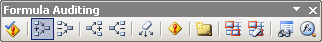
The buttons on the Formula Auditing toolbar and their tooltips, from left to right, are listed in Table 3-8.
Table 3-8. The Buttons on the Formula Auditing Toolbar
Button | Action |
|---|---|
Excel starts the error audit to show all errors and their causes (see Figure 3-30 in the next section). | |
The traces from the selected cell to the precedents are marked. To trace additional precedent levels, click the button again. | |
The tracer arrows to the precedent level are removed. If several precedent levels were traced, you have to click this button for each level. | |
The tracer arrows point to all formulas with references to the selected cell. Click again to show tracer arrows at the next level. | |
The tracer arrows to the dependent level are removed. If several dependent levels were traced, you have to click this button for each level. | |
All tracer arrows in the active sheet are removed. | |
Click this button to point tracer arrows to an error source. | |
This button corresponds to the Paste/Comment menu option. | |
Cells or data that don’t meet the specified criteria are marked with a red oval. | |
Click this button to delete the validation circles. You can find more information about validation in Excel help. | |
You can watch the content of selected cells while searching for errors (see Figure 3-31 in the next section). | |
Use this function to resolve formulas step by step. With this analysis process, you can quickly find errors. |


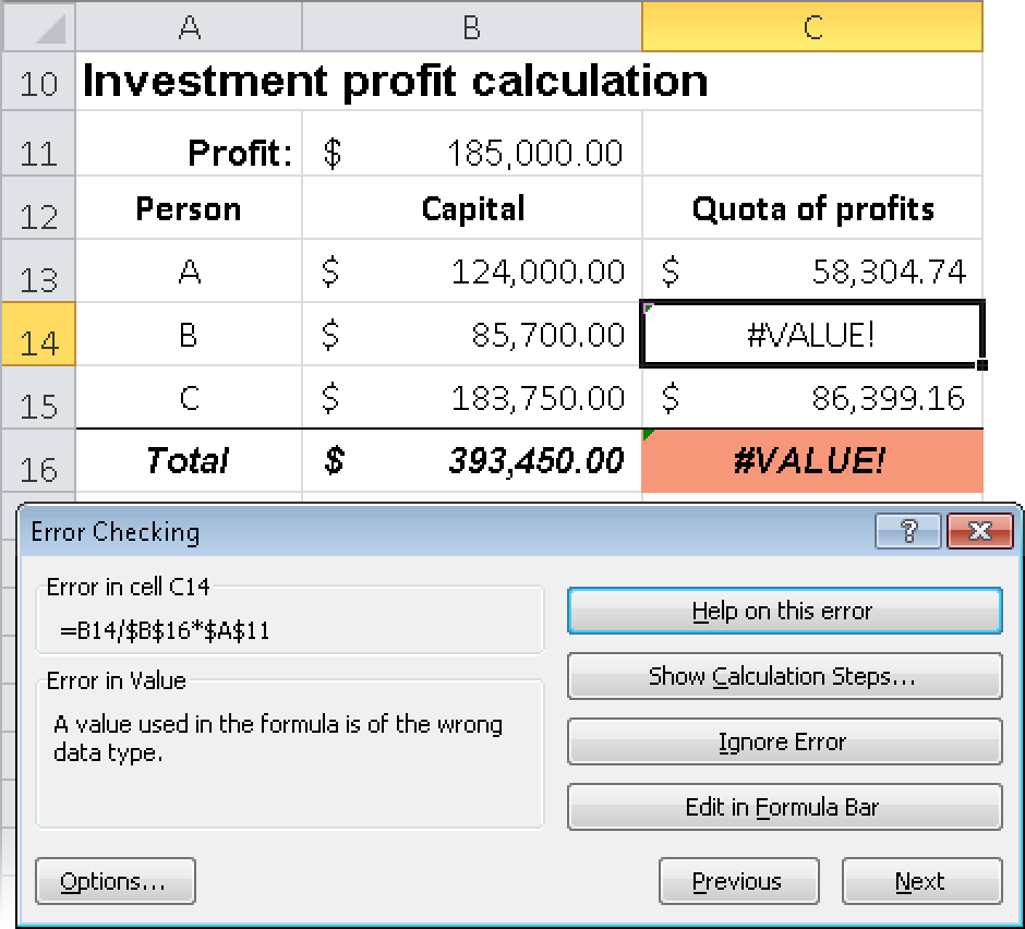
In this example, the calculation results on a worksheet are not the expected results. You want to find out whether the data or the formulas contain errors. Select the error-checking option to start the validation. The dialog box for the first error found appears (see Figure 3-30). Select the next step.
Alternatively, select a cell that has a green triangle in its upper-left corner, and click the Caution symbol. Select the next step in the menu that appears.
Here’s another example: Several calculation steps based on each other don’t return the expected result. You want to watch all intermediate steps. To do this, perform the following steps:
Click the Formula Auditing/Watch Window option. The Watch Window dialog box appears (see Figure 3-31).
Click the Add Watch button and select the first cell with an intermediate calculation. Click Add.
Do the same for all other cells with intermediate calculations.
Change the initial values. The Watch window shows the intermediate calculations.

If you don’t need this window, close it. If you open the window later, the window displays the watched cells again.
The evaluation of formulas is useful in checking for errors, because Excel allows you to resolve the formula step by step.
Select a formula cell and then select Formula Validation/Formula Evaluation. In the dialog box that appears, click the Step In or Step Out button to resolve the formula (see Figure 3-32). This way you can also find out whether your formula includes errors in reasoning not found by Excel.

Note
To control the behavior of the error-checking and formula auditing features, enable or disable the settings on the Error Checking tab (by using the Tools/Option menu option in Excel 2003), or select the Formula category in the Excel Options dialog box (click the Office button in Excel 2007 or the File tab in Excel 2010).
