Syntax. MATCH(lookup_value,lookup_array,match_type)
Definition. This function searches for text, numbers, or logical values within a reference or an array and returns the position.
Arguments
lookup_value (required). The number, a string, a logical value, or a reference to a cell containing a value.
lookup_array (required). A contiguous range of cells consisting of one row or one column, or an array constant.
match_type (optional). Must evaluate to a number (–1, 0, or 1). Determines how the lookup_value is matched in the search array. If this argument is omitted, Excel uses the value 1.
The match_type argument is set as follows:
If match_type is –1, the MATCH() function returns the position of the smallest value greater than or equal to lookup_value. The elements in the search array should be sorted in descending order: numbers, letters, then logical values.
If match_type is 0, the MATCH() function returns the position of the first value equal to lookup_value. The elements in the search array do not need to be sorted.
If match_type is 1, the MATCH() function returns the position of the largest value smaller than or equal to lookup_value. The elements in the search array should be sorted in ascending order: first the numbers, then the letters in alphabetical order, and finally the logical values FALSE and TRUE.
Background. Unlike the LOOKUP() function, the MATCH() function determines positions rather than values.
The function returns the #N/A error if no matching value is found. This error is also returned if the lookup_value argument does not correspond to a row or column. If you don’t set the match_type parameter to correspond with the search array, this error is returned even if the value you search for exists in the list.
For a list containing strings, you usually set match_type to 0. In a list containing numbers in intervals (such as discounts, interest rates, or scores), the search array is ascending or descending.
If match_type is 0 and the lookup_value is a string, it can contain the * placeholder for any string and the ? for single characters. The MATCH() function is not case-sensitive.
Examples. The following examples show how this function is used.
Search in Multiple Columns. With the MATCH() function, you can quickly search multiple columns. Assume that you have a price list for clothing (see Figure 10-6).
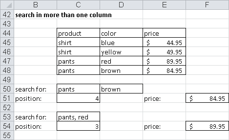
You can determine the position of the yellow shirt with the formula
{=MATCH(C50 & D50,C45:C48 & D45:D48,0)}Because this is an array formula, you have to press Ctrl+Shift+Enter after entering the formula. The & links elements in the lookup_value and combines the two search columns into one column.
The INDEX() function returns the price:
=INDEX(E45:E48,C51)
Of course, you can combine both formulas into a single formula:
{=INDEX(E45:E48,MATCH(C50 & D50,C45:C48 & D45:D48,0))}To enter the search criteria in a single row (C53 in Figure 9-9), use the following formula:
{=MATCH(C53,C45:C48 & ", " & D45:D48,0)}This is also an array formula. The search columns are now combined.
You can use the placeholders to find the elements even if you know only part of their names. If you enter pa in C58 and re in D58, the formula
{=MATCH("*" & C58 & "*" & D58 & "*",C45:C48 & D45:D48,0)}finds the row containing the red pants.
Note
Because such a formula can get quite complicated, you should consider using Advanced Filter. If you copy the table ranges to another location (instead of filtering the list in place), the copy is independent of the original table and not updated simultaneously.
Cross Tabulations in Practice. Cross tabulations (the simplest form of PivotTable) are often used. These include tables such as time tables, distances between cities, and rate tables. Assume that you have a phone rate comparison table that tells you who the cheapest provider is at certain times of the day. Figure 10-7 shows an example.

Looking for a time in the left column is a job for MATCH(). But what column contains the result? Use the MATCH() function to find the row, and the MIN() and OFFSET() functions to find the cheapest rate. Here is the MATCH() function:
=MATCH(C81,B75:B79,1)
And here are the MIN() and the OFFSET() functions:
=MIN(OFFSET(C75:E79,C82-1,0,1,3))
You can combine both formulas into one. Thus, the following formula locates the provider who offers the cheapest rate:
=INDEX(C74:E74,1,MATCH(C83,OFFSET(C75:E79,C82-1,0,1,3),0))
OFFSET() finds the correct row (with the first number being 0); C83 contains the cheapest rate returned by MATCH(), and INDEX() searches the header for the provider.
Tip: Select a row using conditional formatting
To select the row with the cheapest rate, use conditional formatting. In C75 enter the following formula:
=AND(C75=MIN(OFFSET($C$75:$E$79,MATCH($C$81,$B$75:$B$79,1)-1,0,1,3)),
   (ROW(C75)-ROW($C$75)+1)=$C$82)
This formula checks whether the cell contains the cheapest rate in the correct row. Select a color, and copy the format by using Paste Format.