AGGREGATE()

Syntax. This function has two forms:

• AGGREGATE(function_num, options, ref1, ref2,...) (reference form)

• AGGREGATE(function_num, options, array, k) (array form)

Definition. This function returns an aggregate in a list or database.

Arguments

• function_num (required) A number between 1 and 19 that specifies the function to use (see Table 16-2).

  Table 16-2. Possible Values for the function_num Argument

  function_num	Function
  1	AVERAGE()
  2	COUNT()
  3	COUNTA()
  4	MAX()
  5	MIN()
  6	PRODUCT()
  7	STDEV.S()
  8	STDEV.P()
  9	SUM()
  10	VAR.S()
  11	VAR.P()
  12	MEDIAN()
  13	MODE.SNGL()
  14	LARGE()
  15	SMALL()
  16	PERCENTILE.INC()
  17	QUARTILE.INC()
  18	PERCENTILE.EXC()
  19	QUARTILE.EXC()

• options (required) A numerical value that determines which values to ignore in the evaluation range (see Table 16-3).

  Table 16-3. Possible Values for the option Argument

  option	Behavior
  0 or omitted	Ignores nested SUBTOTAL() and AGGREGATE() functions
  1	Ignores hidden rows and nested SUBTOTAL() and AGGREGATE() functions
  2	Ignores error values and nested SUBTOTAL() and AGGREGATE() functions
  3	Ignores hidden rows, error values, and nested SUBTOTAL() and AGGREGATE() functions
  4	Ignores nothing
  5	Ignores hidden rows
  6	Ignores error values
  7	Ignores hidden rows and error values

• ref1 (reference form, required) The first numeric argument for functions that use multiple numeric arguments for which you want the aggregate value.

• ref2 (reference form, optional) At least two and up to 253 arguments for which you want the aggregate value.

  For functions that take an array, ref1 is an array, an array formula, or a reference to a range of cells for which you want the aggregate value. ref2 (k) is a second argument that is required for certain functions. The following functions require a ref2 argument:

  • LARGE(array,k)

  • SMALL(array,k)

  • PERCENTILE.INC(array,k)

  • QUARTILE.INC(array,quart)

  • PERCENTILE.EXC(array,k)

  • QUARTILE.EXC(array,quart)

Note

If a second ref argument is required but not specified, the AGGREGATE() function returns the #VALUE! error. If one or more of the references is a 3-D reference, then AGGREGATE() returns the #VALUE! error.

If the references include additional AGGREGATE() functions, the nested functions could be ignored, so they are not considered multiple. The same applies if the references contain subtotals.

Remember: The AGGREGATE() function is intended for data columns or vertical ranges, not for rows or horizontal ranges. Hiding a column doesn’t affect the result. However, if you hide a row, the result is different.

Background. The AGGREGATE() function is very powerful. This function was added to Excel 2010 to remove some restrictions the other functions have. Most functions return an error if the calculated references are incorrect. In such cases in the previous Excel versions, you had to run a complex IFERROR() query. With the AGGREGATE() function you can also control the behavior of hidden cells.

The AGGREGATE() function allows you to calculate formulas for value ranges with subtotals without including the subtotals in the result. See Figure 16-4 for an example of when this function could be useful.

Figure 16-4. The SUBTOTAL() function cannot ignore the errors.

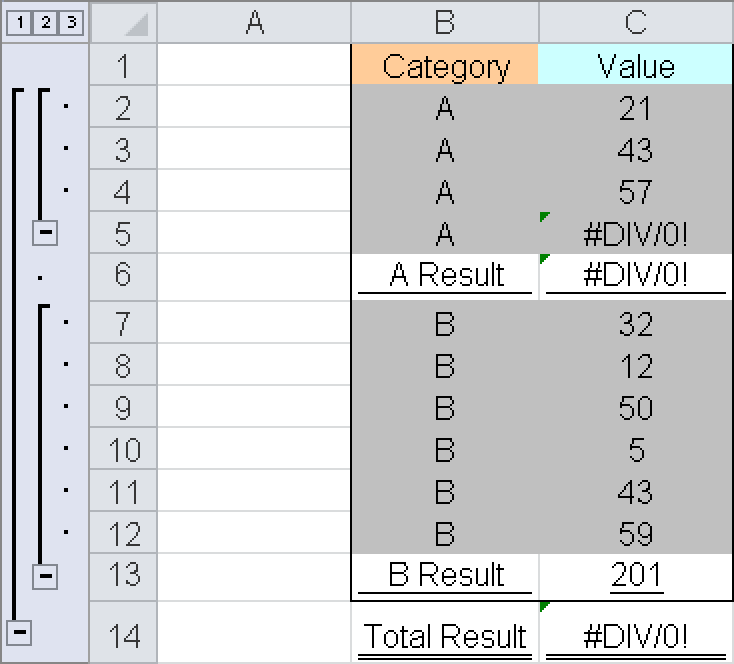
In the figure, the SUM() and SUBTOTAL() functions cannot add the values in column C. However, the formula

=AGGREGATE(9,3,C18:C29)

returns a useful result despite the error and the subtotals. You can also ignore hidden cells so that you only add the values in the visible range. With only one click, you can include entire ranges in the result or hide them.

Example. This function is used for numerous purposes, such as a series of measurements for which the total is calculated regardless of errors or subtotals.

See Also

SUBTOTAL()

Sample Files

Use the AGGREGATE.xlsx. The sample files are found in the Chapter16 folder. For more information about the sample files, see the section titled Using the Sample Files.