CHAPTER 10

Raster GIS

LEARNING GOALS

• Extract and symbolize raster maps.
• Create hillshade maps.
• Smooth point data with kernel density smoothing.
• Build a raster-based risk index.
• Build a model for automatically creating risk indices.

Introduction

Thus far, this book has been devoted to vector feature classes (points, lines, and polygons), except for displaying the raster basemaps available in ArcGIS Pro, plus an occasional raster map layer. Vector feature classes are useful for discrete features (such as streetlight locations, streets, and city boundaries). Raster map layers are best suited for continuous features (for example, satellite images of Earth, topography, and precipitation). Raster map layers also can be used when you want to display large numbers of vector features (for example, all blocks in a city, all counties in the United States). In some cases, you have so many vector features that the features of choropleth and other maps are too small to render clearly. In such cases, as you will see in this chapter, you can transform vector feature classes into raster datasets that you can easily visualize. This chapter first presents some background on raster maps before discussing exactly what you’ll be doing next.

Raster dataset is the generic name for a cell-based map layer stored on a disk in a raster data format. Esri supports more than 70 raster dataset formats, including familiar image formats such as TIFF and JPEG, as well as GIS-specific formats such as Esri Grid. You can import raster datasets into file geodatabases.

All raster datasets are arrays of cells (or pixels)—each with a value and location, and rendered with a color when they are mapped. Of course, just like any other digital image, the pixels are so small at intended viewing scales that they are not individually distinguishable. The coordinates for a raster dataset are the same kind as used for vector maps (chapter 5).

All raster datasets have at least one band of values. A band is comparable to an attribute for vector map layers but stores the values of a single attribute in an array. The values can be positive or negative integers or floating-point numbers. You can use integer values for categories (codes), which must have a layer file with descriptions and colors (for example, 1 = Agriculture, brown; 2 = Forest, green). Raster dataset values can also be floating-point numbers representing magnitudes (for example, temperature and slope steepness of terrain).

Color capture and representation in raster datasets is an important topic. Color in the visible range is captured by satellites in three bands (for example, red, blue, and green) that mix to produce any color. Color in many raster datasets, however, is often represented in one band using a color map, in which each color is given a code (integer value). Color depth is the term given to the number of bits for code length (on/off switches in data storage) used to represent colors. So-called “true color” uses 24 bits per pixel and can represent more than 16 million colors (the human eye can distinguish about 10 million colors).

The spatial resolution of a raster dataset is the length of one side of a square pixel. So if a pixel is 1 meter on a side, it has 1 meter spatial resolution (which is a high resolution leading to high-quality maps). The US Geological Survey provides imagery for urban areas in the United States at this resolution or higher with images capable of being zoomed far into small parts of neighborhoods (for example, with driveways, swimming pools, and tennis courts being clearly shown when displayed). The current Landsat 7 and 8 satellites that together image the entire Earth every eight days have a resolution of 30 meters for most of their eight bands, which is good for viewing areas as small as neighborhoods of a city.

File sizes for raster datasets can be very large, requiring large amounts of disk space for storage, and also taking potentially relatively long times to process and display on a computer screen. Raster GIS uses several mechanisms to reduce storage and processing time, including data compression and pyramids. Pyramids provide additional raster layers with larger spatial resolutions for zoomed-out viewing that take less time to display than the original layer. A mosaic dataset is a data catalog for storing, managing, viewing, and querying collections of raster datasets, often forming a continuous map when viewed. Although such a mosaic dataset is viewed as a single mosaicked image, you also have access to each dataset in the collection. A mosaic dataset also can store raster datasets of the same area for different times, with viewing of any time period’s map and comparing different time periods.

 

Tutorial 10-1: Process raster datasets

The ArcGIS Pro project that you will open has single-band raster datasets for land use and elevation, downloaded from the US Geological Survey’s website. You’ll extract raster datasets for Pittsburgh from each original dataset that has extents larger than Pittsburgh’s. Because raster datasets are rectangular, you’ll display layers using Pittsburgh’s boundary as a mask: pixels in Pittsburgh’s rectangular extent but outside the city’s boundary will still exist but will be given no color, while those within Pittsburgh will have assigned colors. Finally, you’ll use the elevation layer to produce a hillshade layer, which is a shaded relief rendering of topography created by using an artificial sun to add illumination and shadows.

Open the Tutorial 10-1 project

1. 1.Open Tutorial10-1 from the Chapter10\Tutorials folder, and save it as Tutorial10-1YourName.
2. 2.Use the Raster datasets bookmark. National Elevation Dataset (NED) is elevation data, and it will look like topography after you create a hillshade for it. LandUse_Pgh has land-use categories but must have its layer file applied to get its color map and code descriptions for interpretation.

Examine raster dataset properties

Raster datasets have considerable metadata that you can read as properties.

1. 1.In the Contents pane, right-click NED, and click Properties > Source. The dataset is in the Chapter10.gdb file geodatabase, where the dataset was imported from its original raster format. The elevation units are in feet above sea level.
2. 2.Click Raster information. The raster dataset has one band with 1,984 rows and 2,106 columns, for a total of 4,178,304 cells. The cells have roughly 90-foot (30-meter) resolution. The raster has pyramids for speedy display when zooming out.
3. 3.Scroll down and click Statistics. The average elevation in the raster dataset is 323.7 feet, with a minimum of 206.9 feet and a maximum of 443.2 feet above sea level.
4. 4.Click Extent. The four values provided are state plane coordinates in feet that you can use to specify the four corners of the rectangular extent of the raster dataset.
5. 5.Click Spatial Reference. Here you see that the coordinates are in state plane feet for southern Pennsylvania, which uses a Lambert Conformal Conic projection tuned for southern Pennsylvania.
6. 6.Click Cancel.

YOUR TURN

Review the properties of LandUse_Pgh. Notable are that the raster format is TIFF, a common image format. Its resolution is 30 meters, with a single band and a color map (which is available in a separate layer file that you’ll use in an exercise that follows). It has a projection for the lower 48 states (Albers Equal Area) that distorts direction (which explains why it’s tilted).

Import a raster dataset into a file geodatabase

Next, you’ll import LandUse_Pgh.tif into the Chapter10.gdb file geodatabase.

1. 1.On the Analysis tab, click Tools.
2. 2.In the Geoprocessing pane, search for and open the Raster To Other Format tool.
3. 3.For the Input rasters field, browse to Chapter10\Data, select LandUse_Pgh.tif, and click OK.
4. 4.For Output workspace, browse to Chapter10\Tutorials, select Chapter10.gdb, and click OK.
5. 5.For Raster format, select Esri Grid, run the tool, and close it when it finishes.
6. 6.Remove LandUse_Pgh.tif from the Contents pane, add LandUse_Pgh from Chapter10.gdb, and move it below NED in the Contents pane. Nothing appears to change on the map, but the source of LandUse_Pgh is now the Esri Grid.

Set the geoprocessing environment for raster analysis

Environmental settings affect how geoprocessing is carried out by tools in the current project. You’ll set the cell size of raster datasets you create to 50 feet, and you’ll use Pittsburgh’s boundary as the default mask.

1. 1.On the Analysis tab, click Environments.
2. 2.In the Environments settings for the Raster Analysis category, type 50 for Cell Size, and select Pittsburgh for the default mask.
3. 3.Click OK.

Extract land use using a mask

Next, you’ll use the Extract By Mask tool to extract LandUse_Pittsburgh from LandUse_Pgh. The resulting raster dataset will have the same extent as Pittsburgh and therefore be a much smaller file to store than the original.

1. 1.In the Geoprocessing pane, search for and open the Extract By Mask tool.
2. 2.Type or make the selections as shown. Note that the Extract By Mask tool has you specify the mask layer explicitly, in case you want to override the default mask you set in Environments.

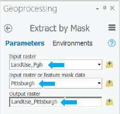
1. 3.Click Run, and close the Geoprocessing pane when the tool is finished. ArcGIS Pro applies an arbitrary color scheme to the new layer.
2. 4.Remove LandUse_Pgh from the Contents pane.
3. 5.Open the Catalog pane, expand Databases and Chapter10.gdb, right-click LandUse_Pgh, and click Delete > Yes.
4. 6.Use the Pittsburgh bookmark.

YOUR TURN

Extract NED_Pittsburgh from NED using the Extract By Mask tool. In the Geoprocessing pane, for Extract by Mask, click Environments and then the Select coordinate system button on the right of Output Coordinate System. Expand Projected coordinate system > State Plane, NAD 1983 (US Feet), select the projection for Pennsylvania South, and click OK. Then on the Parameters tab, select NED as input raster, Pittsburgh as the mask, and NED_Pittsburgh as the output raster, and run the tool. After creating NED_Pittsburgh, remove NED from the map and delete it from Chapter10.gdb.

Symbolize a raster dataset using a layer file

1. 1.Open LandUse_Pittsburgh’s Symbology pane, and click the Menu button > Import symbology.
2. 2.Browse to Chapter10\Data, double-click LandUse.lyr, and turn off NED_Pittsburgh.
3. 3.In the Contents pane, expand LandUse_Pgh to see land-use categories and their colors. The code values stored in the raster’s band are integers, and you can see them by looking at the layer’s Symbology pane.

1. 4.Close the Symbology pane.

Create hillshade for elevation

Hillshade provides a way to visualize elevation. The Hillshade tool simulates illumination of the earth’s elevation surface (the NED raster layer) using a hypothetical light source representing the sun. Two parameters of this function are the altitude (vertical angle) of the light source above the surface’s horizon in degrees and its azimuth (east–west angular direction) relative to true north. The effect of hillshade to elevation is striking because of light and shadow. You can enhance the display of another raster layer, such as land use, by making land use partially transparent and placing hillshade beneath it. You’ll use the default values of the Hillshade tool for azimuth and altitude. The sun for your map will be in the west (315°) at an elevation of 45° above the northern horizon.

1. 1.Search for and open the Hillshade (Spatial Analyst Tools) tool.
2. 2.Type or make the selections as shown.

1. 3.Run the tool, and close it when it finishes.

Symbolize hillshade

The default symbolization of hillshade can be improved upon, as you’ll do next.

1. 1.Open the Symbology pane for Hillshade_Pittsburgh.
2. 2.Type or make the selections as shown.

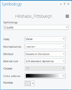
1. 3.Close the Symbology pane. The Hillshade looks better, although you can see the 30 m pixels of the layer.

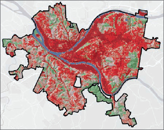
Use hillshade for shaded relief of land use

Next, you’ll make LandUse_Pittsburgh partially transparent and place Hillshade_Pittsburgh beneath it to give land use shaded relief.

1. 1.Move LandUse_Pittsburgh above Hillshade_Pittsburgh, turn on LandUse_Pittsburgh, and turn off NED_Pittsburgh (if it’s on).
2. 2.With LandUse_Pittsburgh selected in the Contents pane, on the Raster Layer contextual tab, click Appearance.
3. 3.In the Effects group, move the Layer Transparency slider to 33.0 %. Hillshade_Pittsburgh shows through the partially transparent LandUse_Pittsburgh, giving the land-use layer a rich, 3D-like appearance.

Create elevation contours

Another way to visualize elevation data—elevation contours—is with lines of constant elevation, as commonly seen on topographic maps. For Pittsburgh, the minimum elevation is 215.2 feet and the maximum is 414.4 feet, with about a 200-foot difference. If you specify 20-foot contours, starting at 220 feet, there will be about 10 contours. Note that the output contours are vector line data (and not polygon data).

1. 1.In the Geoprocessing pane, search for and open the Contour (Spatial Analyst) tool.
2. 2.Type or make your selections as shown. The Z factor can be used to change units. For example, if the vertical units were meters, you would enter 3.2808 to convert to feet. We’ll leave the value at 1, because the vertical dimensions are already in the desired units of feet.

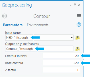
1. 3.Run the tool, and close the Geoprocessing pane when the tool is finished.
2. 4.Turn off LandUse_Pittsburgh and Hillshade_Pittsburgh.
3. 5.Open the Symbology pane for Contour_Pittsburgh, and use Single Symbols for Symbology with a medium-gray line of width 0.5. Note that you could label contours with their contour elevation values when zoomed in, but you will not do that in this exercise.

1. 6.Save and close your project.

 

Tutorial 10-2: Make a kernel density (heat) map

Kernel density smoothing (KDS) is a widely used method in statistics for smoothing data spatially. The input is a vector point layer, often centroids of polygons for population data or point locations of individual demands for goods or services. KDS distributes the attribute of interest of each point continuously and spatially, turning it into a density (or “heat”) map. For population, the density is, for example, persons per square mile.

KDS accomplishes smoothing by placing a kernel, a bell-shaped surface with surface area 1, over each point. If there is population, N, at a point, the kernel is multiplied by N so that its total area is N. Then all kernels are summed to produce a smoothed surface, a raster dataset.

The key parameter of KDS is its search radius, which corresponds to the radius of the kernel’s footprint. If the search radius is chosen to be small, you get highly peaked “mountains” for density. If you choose a large search radius, you get gentle, rolling hills. If the chosen search radius is too small (for example, smaller than the radius of a circle that fits inside most polygons that generate the points), you will get a small bump for each polygon, which does not amount to a smoothed surface.

Unfortunately, there are no really good guidelines on how to choose a search radius, but sometimes you can use a behavioral theory or craft your own guideline for a case at hand. For example, crime hot spots (areas of high crime concentrations) often run the length of the main street through a commercial corridor and extend one block on either side. In that case, we use a search radius of one city block’s length.

Open the Tutorial 10-2 project

The map in this tutorial has the number of myocardial infarctions (heart attacks) outside of hospitals (OHCA) during a five-year period by city block centroid. One of the authors of this book studied this data to identify public locations for defibrillators, devices that deliver an electrical shock to revive heart attack victims. One location criteria was that the devices be in or near commercial areas. Therefore, the commercial area buffers are commercially zoned areas, plus about two blocks (600 feet) of surrounding areas.

KDS is an ideal method for estimating the demand surface for a service or good, because its data smoothing represents the uncertainty in locations for future demand, relative to historical demand. Also in this case, heart attacks, of course, do not occur at block centroids, so KDS distributes heart attack data across a wider area.

1. 1.Open Tutorial10-2 from EsriPress\GIST1Pro\Exercises\Chapter10 and save it as Tutorial10-2YourName.
2. 2.Use the Pittsburgh bookmark.

Run KDS

Blocks in Pittsburgh average about 300 feet per side in length. Suppose that health care analysts estimate that a defibrillator with public access can be identified for residents and retrieved for use as far away as 2½ blocks from the location of a heart attack victim. They thus recommend looking at areas that are five blocks by five blocks in size (total of 25 blocks or 0.08 square miles), 1,500 feet on a side, with defibrillators located in the center. With this estimate in mind, you’ll use a 1,500-foot search radius to include data within reach of a defibrillator, plus data beyond reach to strengthen estimates.

The objective is to determine whether Pittsburgh has areas that are roughly 25 blocks in area and, as specified by policy makers, have an average of about five or more heart attacks a year outside of hospitals.

1. 1.Search for and open the Kernel Density tool.
2. 2.Click Environments, and for Cell size, type 50, and for Mask, select Pittsburgh. Note that environment settings made in the tool apply only to running the tool itself and not to other tools, such as when you set Environments on the Analysis tab.
3. 3.Click Parameters, and type or make the selections as shown.

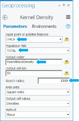
1. 4.Run the tool, and close it when it finishes.
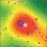
2. 5.Turn off the OHCA and Commercial Area Buffer layers to see the smoothed layer. The default symbolization is not effective in this case, so next you’ll resymbolize the layer.
3. 6.Change the smoothed layer’s symbology to use Classify as Symbology, Standard Deviation for method with ¼ standard deviation interval size, and the green to yellow to red color scheme.
4. 7.Close the Symbology pane. The smoothed surface provides a good visualization of the OHCA data, whereas the original OHCA points, even with size-graduated point symbols for number of heart attacks, are difficult to interpret. Try turning the OHCA layer on and off to see the correspondence between the raw-versus-smoothed data. Note that the densities are in heart attacks per square mile and that the maximum is nearly 1,000 per square mile over five years. Although seemingly large, a square mile is a very large area in a city. The target area of 25 blocks is only 0.08 square miles. Also, only a small part of Pittsburgh (and much less than a square mile) has a density of nearly 1,000 heart attacks per square mile.

1. 8.Save your project.

Create a threshold contour layer for locating a service

Assuming that target areas will be around a tenth of a square mile in area, suppose policy makers decide on a threshold of 250 or more heart attacks per square mile in five years (or 50 per square mile per year). Next, you’ll create vector contours from the smoothed surface to represent this policy.

1. 1.Search for and open the Contour List (Spatial Analyst) tool.
2. 2.Make the selections or type as shown. You’ll create only one contour, 250, for the threshold defining a target area.

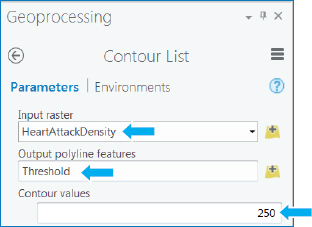
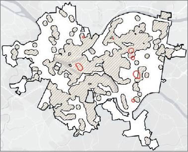
1. 3.Run the Contour List tool, close the tool when it finishes, turn off HeartAttackDensity and Rivers, and turn on Commercial Area Buffer. Relatively few areas—seven—meet the criterion, and three of those areas appear quite small. All seven threshold areas are in or overlap commercial areas, so you can consider all seven as potential sites for defibrillators. Do any of the areas have the expected number of heart attacks per year to warrant defibrillators? The next exercise addresses this question. Turn the Commercial Area Buffer off.

Estimate the number of annual heart attacks using threshold areas

To estimate annual heart attacks, you can select OHCA centroids within each threshold area, sum the corresponding number of heart attacks, and divide by 5 since OHCA is a five-year sample of actual heart attacks. You will use the Threshold boundaries in a selection by location query, in which case the Threshold layer must be polygons. However, if you examine the properties of the Threshold layer, you’ll see that it has the line vector type and not polygon type, even though all seven areas look like polygons. The tool you ran to create Thresholds creates lines because some peak areas of an input raster could overlap with the border of the mask—Pittsburgh, in this case. The lines for such cases would not be closed but left open at the border. Nevertheless, ArcGIS Pro has a tool to create polygons from lines that you’ll use next.

1. 1.In the Geoprocessing pane, search for and click the Feature To Polygon tool.
2. 2.Type or make the selections as shown.

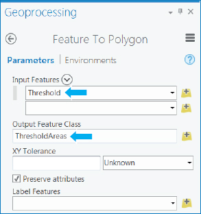
1. 3.Run the tool, and close the tool after it finishes.
2. 4.Search for the Summarize Within tool, and make the following selections as shown. In effect, this tool runs the Summary tool several times—in this case, once for each polygon in the ThresholdAreas feature class to calculate corresponding statistics in the OHCA feature.

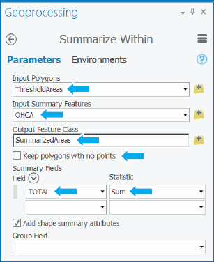
1. 5.Run the tool, and close the tool after it finishes.
2. 6.Open the SummarizeAreas attribute table, and sort it by Sum Total descending. One of the ThresholdAreas polygons had no OHCA points inside the polygon but was surrounded by points that contributed its peak density. Clearing the “Keep polygons with no points” check box eliminated that polygon from being summarized. The best candidate for a defibrillator has an annual average of 104/5 = 20.8 heart attacks per year and is not in the central business district (CBD) but is the large area on the east side of Pittsburgh. The CBD is in the second row with an average of 68/5 = 13.6 heart attacks per year. The last row’s area is the only one that does not meet the criterion of at least five heart attacks per year on average, with 4.2.

Next, you will find the ThresholdAreas polygon that has no OHCA points and is not included in the previous table. The polygon (pink fill color) is about a city block in size and is predicted to be the peak density area on the basis of contributions from the kernels of nearby OHCA points, but it has no points itself! Given the polygon’s small size, its 28 nearby heart attacks in the five-year sample, and its distance within five blocks of the peak area, perhaps the polygon also warrants consideration as a defibrillator site.

 

Tutorial 10-3: Building a risk index model

In this tutorial, you learn more about creating and processing raster map layers. You also are introduced to ArcGIS Pro’s ModelBuilder to build models. A model, also known as a macro, is a computer script that you create without writing computer code (a script runs a series of tools). Instead of writing computer code, you drag tools to the model’s canvas (editor interface) and connect them in a workflow. Then ArcGIS Pro writes the script in the Python scripting language. Ultimately, you can run your model just as you would any other tool.

The model that you will build in this tutorial calculates an index for identifying poverty areas of a city by combining raster maps for these poverty indicators:

• Population below the poverty income line
• Female-headed households with children
• Population 25 or older with less than a high school education
• Number of workforce males 16 or older who are unemployed

Low income alone is not sufficient to identify poverty areas, because some low-income persons have supplemental funds or services from government programs or relatives, and so rise above the poverty level. Female-headed households with children are among the poorest of the poor, so these populations must be represented when you consider poverty areas. Likewise, populations with low educational attainment and/or low employment levels can help identify poverty areas.

Dawes¹ provides a simple method for combining such indicator measures into an overall index. If you have a reasonable theory that several variables are predictive of a dependent variable of interest (whether the dependent variable is observable or not), Dawes contends that you can proceed by removing scale from each input and then average the scaled inputs to create a predictive index. A good way to remove scale from a variable is to calculate z-scores, subtracting the mean and then dividing by the standard deviation of each variable. Each standardized variable has a mean of zero and standard deviation of one (and therefore no scale).

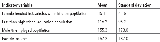
Table 10-1 for Pittsburgh block groups shows that if you simply averaged the four variables, the variable female-headed households would have a small weight, given its mean of only 36.1, while the means of the other three variables are all higher than 100. Z-scores level the playing field so that all variables have an equal role.

Table 10-1

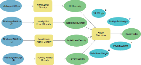
The workflow to create the poverty index has three steps:

1. 1.Calculate z-scores for each of the four indicators.
2. 2.Create kernel density maps for all four z-score variables. Although you need the kernel density maps as input to the third step, you should also study them individually to understand their spatial patterns in relationship to the poverty index.
3. 3.Use a tool to average the four weighted raster surfaces and create the index raster layer.

Experts/stakeholders in the policy area using the raster index can judgmentally give more weight to some variables than others if they choose. They must only use nonnegative weights that sum to one (1). So if judgmental weights for four input variables are 0.7, 0.1, 0.1, and 0.1, then the first variable is seven times more important than each of the other three variables. With different stakeholders possibly having different preferences, having a macro would allow you to repeatedly run the macro with different sets of weights for the multiple-step process for creating an index raster layer. For example, some policy makers (educators and grant-making foundations) may want to emphasize unemployment or education and give those inputs more weight than others, whereas other stakeholders (human services professionals) may want to heavily weight female-headed households.

Standardizing the input variables need only be done once, so you’ll do that step manually, but then you’ll complete parts 2 and 3 of the workflow using a ModelBuilder model for creating indexes.

Open the Tutorial 10-3 project

All input variables must come from the same point layer (block group centroids, in this case) as input to build the index so that the data standardization and averaging process is valid. You’ll use a 3,000-foot buffer of the study region (Pittsburgh) for two purposes.

First, KDS uses the northernmost, easternmost, southernmost, and westernmost points of its input point layer to define its extent. If the inputs are polygon centroids in a study region, the corresponding KDS raster map will be cut off and not quite cover the study region. The block group centroids added by the buffer yield KDS rasters that extend a bit beyond Pittsburgh’s border, but the Pittsburgh mask will show only the portion within Pittsburgh.

Second, in applying KDS, the buffer eliminates the boundary problem for estimation caused by abruptly ending data at the city’s edge. KDS estimates benefit from the additional data provided by the buffer beyond the city’s edge.

1. 1.Open Tutorial10-3 from EsriPress\GIST1Pro\Exercises\Chapter10, and save it as Tutorial10-3YourName.
2. 2.Use the Pittsburgh bookmark.

Standardize an input attribute

PittsburghBlkGrps already has three out of four input attributes standardized and ready to use in the poverty index you’ll compute, but FHHChld has not yet been standardized. For practice purposes, you will standardize this attribute next.

1. 1.Open the attribute table of PittsburghBlkGrps, and scroll to the right to see FHHChld (female-headed household with children).
2. 2.Right-click the FHHChld column header, click Summarize, and type or make the selections as shown. Be sure to click on the left of the case field, and click its red X to clear it.

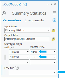
1. 3.Run the tool, close the Geoprocessing pane when the tool is finished, close the attribute table, and open the output table, PittsburghBlkGrps_Statistics. Rounded to one decimal place, the mean of FHHChld is 36.1, and its standard deviation is 41.6.
2. 4.In the Contents pane, right-click PittsburghBlkGrps, and click Design > Fields.
3. 5.Scroll to the bottom of the Fields table, and click to add a new field.
4. 6.Type ZFHHChld for Field name, select Float for Data type, click Save, and close Fields.
5. 7.In the PittsburghBlkGrps attribute table, right-click the ZFHHChld column heading, click Calculate Field, create the expression for ZFHHChld, and click Run. As a check, the ZFHHChld value for the record for ObjectID = 1 is –0.146635.
6. 8.Close the Geoprocessing window and the attribute table, and save your project.

Set the geoprocessing environment for raster analysis

You’ll set the cell size of rasters you create to 50 feet, and you’ll use Pittsburgh’s boundary as a mask.

1. 1.On the Analysis tab, click Environments.
2. 2.In the Raster Analysis section of Environments, type 50 for Cell Size, and select Pittsburgh for the mask.
3. 3.Click OK.

Create a new toolbox and model

A toolbox is just a container for models (macros). When your project was created, ArcGIS Pro built a toolbox, named Chapter10.tbx, which is where your model will be saved.

1. 1.On the Analysis tab in the Geoprocessing group, click ModelBuilder.
2. 2.Open the Catalog pane, expand Toolboxes, expand Chapter10.tbx, right-click Model, and click Properties.
3. 3.For Name, type PovertyIndex (with no blank space between the two words); for Label, type Poverty Index; and click OK.
4. 4.Hide the Catalog pane.
5. 5.On the ModelBuilder tab in the Model group, click Save.

Add processes to the model

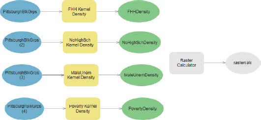
ModelBuilder has a drag-and-drop environment: you’ll search for tools, and when you find them, you’ll drag them to your model, open their input/output/parameter forms, and fill the forms out.

1. 1.Search for, but do not open, the Kernel Density tool.
2. 2.Drag the Kernel Density tool to your model.
3. 3.Drag the model and its output to the upper center of the model window, and click anywhere in the model’s white space to deselect Kernel Density and its output. You’ll need a total of four kernel density processes, one for each of the four poverty indicators. So, next, you’ll drag the tool to the model three more times.
4. 4.Repeat step 2 three more times, and then arrange your model elements as shown in the figure by dragging rectangles around elements to select them, and then dragging the selections.

1. 5.Close the Geoprocessing pane.
2. 6.Search for the Raster Calculator tool, drag it to the right of your other model components, and close the Geoprocessing pane.

Configure a kernel density process

1. 1.Double-click the first Kernel Density process, type or make the selections as shown, and then click OK. Fully configured processes and their valid inputs and outputs are given color fill as you see now. The 3,000-foot search radius is a judgmental estimate large enough to produce good KDS surfaces at the neighborhood level.

1. 2.Right-click Kernel Density, and rename it FHH Kernel Density.
2. 3.Click the ModelBuilder tab, and save your model.

YOUR TURN

Configure three remaining Kernel Density processes, each with PittsburghBlkGrps as the input, a cell size of 50, and a search radius of 3,000, and with population fields ZNoHighSch, ZMaleUnem, and ZPoverty. Resize model elements to improve readability. The numbers of the input block groups do not have to match those in the figure. ModelBuilder just needs the names of all model elements to be unique. Also, your model may not have separate inputs for each KDS process, but instead may have the same PittsburghBlkGrps input to more than one KDS process. Resize model objects to make them readable and well aligned. Review all four KDS processes to make sure that they have correct z-score variable inputs and a 3,000-foot search radius. Save your model.

Configure the raster calculator process

1. 1.Double-click Raster Calculator, and type and make your selections as shown (double-click density rasters to enter them into the expression). The 0.25 weights serve as default values for running the model unless the user changes them as parameters for each weight that you will add later in this tutorial.

1. 2.Click OK.

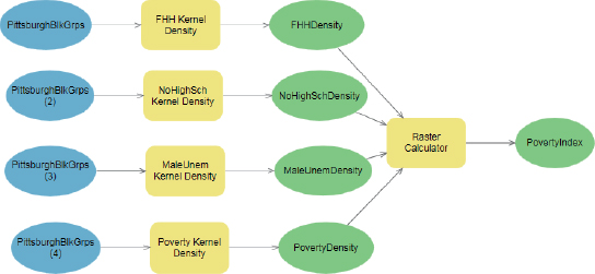
1. 3.Save the model.

Run a model in edit mode

You can run the entire model by clicking its Run button, which you will do next. When you build a model, however, you can run each process one at a time by right-clicking processes and clicking Run, which gives you an ability to isolate errors and fix them. When you finish, you’ll run the model in the Geoprocessing pane.

1. 1.On the ModelBuilder tab in the Run group, click Run. The model runs and produces a log as shown next. If there was an error, the log would give you information about it. Running in edit mode does not add PovertyIndex to the map. You’ll have to add it manually. However, when you run the model as a tool in the Geoprocessing pane, PovertyIndex will be added to the map automatically (when you make PovertyIndex a parameter). If errors arise, you would need to fix them, and then on the ModelBuilder tab in the Run group, you would click Validate and run the model again.

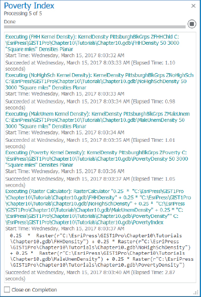
1. 2.Close the log file.
2. 3.In the model, right-click PovertyIndex, and click Add to display.
3. 4.Open your map, and turn off PittsburghBlkGrps. You’ll improve symbolization of PovertyIndex next.

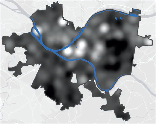
Symbolize a KDS raster layer, and save its layer file

Although vector layers should have a maximum of about seven to nine categories for symbolization of numeric attributes (to avoid a cluttered map and allow easy interpretation using a legend), symbolization of raster layers should have many more categories to represent continuous surfaces. You’ll use standard deviations to create categories and the maximum number of categories with that method. Finally, you’ll save symbolization as a layer file for automatic use whenever the model creates its output, PovertyIndex, with whatever weights the user chooses.

1. 1.Open the Symbology pane for PovertyIndex, select Classify for Symbology, Standard Deviation for Method, ¼ standard deviation for Interval size, and the green to yellow to red Color scheme.

1. 2.With Poverty Index’s Symbology window still open, change the upper value of the largest category from 15.358258 to 100. The change in upper value is a precaution so that if the weights used to run the model lead to a maximum density greater than 15, the higher-density pixels will fall in this category.
2. 3.Close the Symbology pane.
3. 4.Right-click PovertyIndex, click Save as layer file, and save as PovertyIndex to Chapter10\Tutorials. You’ll use the layer file to symbolize PovertyIndex automatically in future runs of the model.
4. 5.Remove PovertyIndex from the Contents pane.

Add variables to the model

One objective for the PovertyIndex model is to allow users to change the poverty index’s weights. To accomplish this change, you must create variables that will store the weights that the user inputs, and then designate each variable as a parameter input by the user. ModelBuilder automatically creates a user interface for your model (just like the interface for any tool). The user can enter weights for your model in the interface as an alternative to the default equal weights.

1. 1.Open your model. Notice that each process and output has a drop shadow, indicating that it’s been run and is finished.
2. 2.On the ModelBuilder tab in the Run group, click Validate. Validate places all model components in the state of readiness to run again. The drop shadows disappear.
3. 3.On the ModelBuilder tab in the Insert group, click the Variable button, select Variant for Variable data type, click OK, and move the Variant variable above the Raster Calculator process. ArcGIS Pro can determine the actual data type of a variant data type variable from entered values. For example, when you give the variable the value 0.25 in step 4, ArcGIS Pro will treat the value as a numeric variable.
4. 4.Right-click the variable, click Open, type 0.25, and click OK. The value of 0.25 is the default value for running the model if the user does not change it.
5. 5.Right-click the Variant variable, click Rename, type FHHWeight, and press Enter.
6. 6.Right-click FHHWeight, and click Parameter. That action places a letter P near the variable, making the variable a parameter. In other models you might build, consider making the model inputs (the four rasters, in this case) parameters if they can change from run to run. Then users could browse for these parameters when they run the model as a tool.

YOUR TURN

Add three more variant variables, all with value 0.25, and named NoHighSchWeight, MaleUnemWeight, and PovertyWeight. Make each variable a parameter. Save your model.

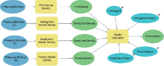
Use in-line variable substitution

In this exercise, you will transfer the weights stored in variables (values that will be input by the user) to parameters of the Raster Calculator tool. The mechanism is called “in-line substitution” because the variables’ values are substituted for the model’s parameter values.

1. 1.Open the Raster Calculator process in the model.
2. 2.Select and then delete the first 0.25 in the expression, leave the cursor in its current position at the beginning of the expression, scroll down in the Rasters pane, and double-click FHHWeight to enter it into the expression where the 0.25 had been.
3. 3.Delete the double quote marks around “%FHHWeight%”.
4. 4.Likewise, select appropriate 0.25 weights for the remaining rasters, yielding the finished expression as follows:
   %FHHWeight% * “%FHHDensity%” + %NoHighSchWeight% * “%NoHighSchDensity%” + %MaleUnemWeight% * “%MaleUnemDensity%” + %PovertyWeight% * “%PovertyDensity%”
5. 5.Click OK. Your Raster Calculator process and its output will get color, and you will validate the process in the next step.
6. 6.On the ModelBuilder tab in the Run group, click Validate.

1. 7.Save your model.

Use a layer file to automatically symbolize the raster layer when created

You’ll use the layer file you created earlier for the poverty index for this task. To do so, you must make the PovertyIndex output of the Raster Calculator process a parameter in the model.

1. 1.Make PovertyIndex a parameter.

   Making PovertyIndex a parameter also adds it to the Contents pane for display in your map when you run the model as a tool from the Geoprocessing pane.

2. 2.Open the Catalog pane, expand Toolboxes > Chapter10, right-click PovertyIndex, and click Properties > Parameters.
3. 3.Scroll to the right, and under the Symbology column heading, click the cell for the row with the label PovertyIndex.
4. 4.In that cell, click the resulting browse button, navigate to Chapter10\Tutorials, and double-click PovertyIndex.lyrx.

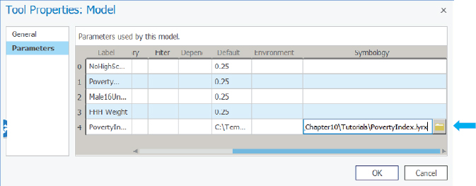
1. 5.Click OK, hide the Catalog pane, and save and close your model.

Run your model

Congratulations, your model is ready to use.

1. 1.With your map open, ensure that PovertyIndex is removed from the Contents pane.
2. 2.On the Analysis tab, click Tools, and search for and open your Poverty Index model.

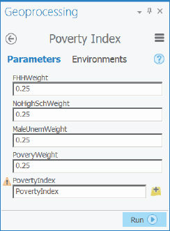
1. 3.Leave the weights at their default settings, and run the model. See that the model computes the poverty index, adds the index to the Contents pane, and symbolizes it with your layer file.
2. 4.Save your project.

YOUR TURN

Remove PovertyIndex from the Contents pane, and try running your model with different weights (nonnegative and sum to one), such as 0.7, 0.1, 0.1, and 0.1. See how the output changes a lot. Note that for a class project or work for a client, you should symbolize PovertyIndex manually to get the best color scheme and categories for a final model, depending on the distribution of densities produced. To do this symbolization, you must go to the model properties and delete the layer file. Otherwise, ArcGIS Pro will not let you change symbolization. When you finish, save your project and close ArcGIS Pro.

Assignments

This chapter has two assignments to complete that you can download from this book’s resource web page, esri.com/gist1arcgispro:

• Assignment 10-1: Create raster maps for the Pittsburgh Almono development area.
• Assignment 10-2: Estimate heart attack fatalities outside of hospitals in Wilkinsburg by gender.

1. 1.Robyn M. Dawes, “The Robust Beauty of Improper Linear Models in Decision Making,” American Psychologist 34, no. 7 (1979) : 571–82.