CHAPTER 11

3D GIS

LEARNING GOALS

• Explore global scenes.
• Learn how to navigate scenes.
• Create local scenes and TIN surfaces.
• Create Z-enabled features.
• Create 3D buildings and bridges from lidar data.
• Work with 3D features.
• Use procedural rules and multipatch models.
• Create an animation.

Introduction

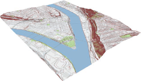
This chapter introduces ArcGIS Pro’s 3D display and processing of data and maps. 3D maps provide insights that are not readily apparent from 2D visualization of the same data. For example, instead of inferring the presence of a valley from 2D contours, in 3D you see the valley and the difference in height between the valley floor and a ridge. 3D maps allow you to design, visualize, communicate, and analyze for better decision-making.

Navigation of ArcGIS Pro in 2D and 3D are similar; however, there are differences when you explore maps with data, such as raster surfaces, lidar data, and 3D features. ArcGIS Pro uses 3D scenes and one of these two viewing modes. The first, global, is for large-extent, real-world content where the curvature of the earth is important. The second, local, is for smaller extent content in a projected coordinate system or cases in which the curvature of the earth isn’t important. You can easily switch scenes between global and local. You can also modify a scene’s settings, depending on the scale of the project. Rendering 3D scenes is slower than rendering 3D maps, and proper computer hardware and configuration is necessary.

This chapter explains procedural methodologies that allow for rapid creation of 3D content. The methodologies describe how to construct multiple 3D models on the basis of feature attributes—such as building heights and roof shape types—rather than creating a single, specific 3D model. Procedural rules, which define patterns, are authored in Esri® CityEngine® a 3D modeling software for urban environments. Procedural rules can be reused in other parts of the ArcGIS platform after they have been exported as rule-package files.

This chapter also explains the use of lidar data and visual analysis tools such as line of sight and introduces 3D animation.

 

Tutorial 11-1: Explore a global scene

Global scenes use a default elevation surface, WorldElevation3D/Terrain3D, from an ArcGIS Online map service. The fixed coordinate system is GCS WGS 1984 and cannot be changed. In this tutorial, you will explore a global scene’s properties and learn how to navigate in 3D. Advantages of the global scene include working in large or multiple geographic areas, enhanced illumination and time effects, and publishing 3D content to a Web Scene.

Open the Tutorial 11-1 project

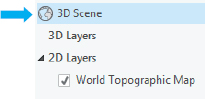
1. 1.Open Tutorial11-1.aprx from Chapter11\Tutorials, and save it as Tutorial11-1YourName.aprx. The project opens with a 3D scene using a default elevation surface, Terrain3D, from an Esri map service. In the Contents pane, 3D Scene is labeled with a globe icon, indicating that it’s a global scene. A global scene whose extent is not clipped includes the entire surface of the earth.

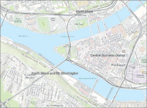
1. 2.Use the Study Area bookmark. The map zooms to a study area of the City of Pittsburgh, including the Central Business District, North Shore, South Shore, and Mount Washington neighborhoods. The map includes no added GIS features yet, just a basemap used as an elevation surface.

Explore a scene’s properties

The scene’s elevation surface is different from a basemap, and understanding the elevation surface, map units, and heights are important in a 3D scene.

1. 1.In the Contents pane, right-click 3D Scene> Properties.
2. 2.In the Map Properties: 3D Scene window, click Elevation Surface, and expand Elevation sources. The scene’s elevation source is visible, showing the elevation Service Name, WorldElevation3D/Terrain3D, and its location from ArcGIS.com.

1. 3.Click General, and under Elevation Units, click Feet, and then click OK. The map and display units will remain decimal degrees for now—only the elevation units change.

Navigate a scene with a mouse and keyboard keys

Next, view the map using a predefined 3D bookmark, and explore using mouse and keyboard shortcuts.

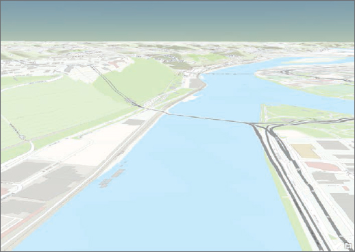
1. 1.Use the Rivers bookmark. The view shows that the terrain is higher in the Mount Washington neighborhood, on the left of the view.

Sometimes, you can get disoriented in a 3D view, so learning a few useful shortcuts can help return you to a familiar orientation. Experiment with the keyboard shortcuts, commonly used to manipulate a 3D view, in the next set of steps.

1. 2.Press and drag the middle mouse button to adjust (tilt) the view.
2. 3.On the keyboard, press the J or U key to move the map up or down.
3. 4.Press the A or D key to rotate the view clockwise or counterclockwise.
4. 5.Press the W or S key to tilt the camera up and down.
5. 6.Press the left, right, up, or down arrow keys to move the view.
6. 7.Press the B key with the left mouse or arrow keys to look around your view.
7. 8.Press the N key to view true North.
8. 9.Press the P key to look straight down at your map.

Change the basemap

Various basemaps can be displayed with the current surface elevation. If you want to see imagery details, they will be draped to the elevation surface.

1. 1.Use the Football Stadium bookmark.
2. 2.Change the basemap to Imagery. The imagery drapes to the elevation surface showing the football stadium, rivers, and trees along the hills above Pittsburgh’s South Shore, and so on.
3. 3.Use the Baseball Stadium bookmark and the mouse or keyboard to see additional views.
4. 4.Change the basemap back to Topographic.

YOUR TURN

Explore another geographic area of the world, perhaps your hometown, your favorite vacation spot, or a city or an area you have always wanted to visit.

Exaggerate and apply a shade and time to a surface

Sometimes, subtle or important changes in the landscape can be emphasized by adding visual effects to the layer. For example, you can graphically exaggerate the height of a mountainous area to help it stand out. This exaggeration does not actually change the elevation but visually makes features more prominent. Another effect includes adding lighting or illumination sources through shading or time of day.

1. 1.Use the Rivers bookmark, open the 3D scene’s properties, and click Elevation Surface.
2. 2.For Exaggeration, type 1.5, and turn on Shade surface relative to the scene’s light position.
3. 3.Click Illumination, click Date and time, and click OK. The elevation will be exaggerated, and the sun shadows are visible and depend on the date and time selected.

YOUR TURN

Pan and navigate the scene to see the exaggeration from different views. Navigate to another area you know is mountainous. Use the Rivers bookmark to return to Pittsburgh. Save your project.

 

Tutorial 11-2: Create a local scene and TIN surface

Advantages of local scenes include using your own elevation surface data such as TIN (triangulated irregular network) or lidar data, using a projected coordinate system, managing features below a surface (for example, subways or water lines), and perhaps more accessibility to edit data. You can also set the coordinate system for a local scene to local coordinates (for example, state plane), and use the surface offline. In this tutorial, you will create a TIN surface from contours, change its symbology, and use it as the elevation surface in a local scene.

Open the Tutorial 11-2 project

1. 1.Open Tutorial11-2.aprx from Chapter11\Tutorials, and save it as Tutorial11-2YourName.aprx. The project opens with a 3D scene named TIN Surface Scene with 2D layer contours, street curbs, parks, and rivers draped to the default Terrain3D elevation surface in a global scene. The basemap is Light Gray Canvas, covering the entire earth. You will convert the global scene to a local scene and clip the basemap to the study area. Unlike the Clip tool, this process “clips” the layers for display purposes only.

Set a local scene

1. 1.On the View tab in the View group, click the Local button . The scene switches from a global to a local scene, and the icon in the Contents pane and on the view updates. Next, you clip the base layer to the study area using the Contours layer.
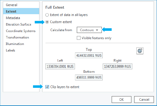
2. 2.In the Contents pane, right-click TIN Surface Scene > Properties > Extent.
3. 3.Click Custom extent, and for Calculate from, click Contours.
4. 4.Turn Clip layers to extent on, and click OK.

1. 5.Use the 3D View bookmark. The basemap will now display only to the extent of the vector features in the study area in the local scene.

Create a TIN surface

A TIN surface is a vector data model composed of irregularly distributed nodes and lines that are formed from x-, y-, and z-values and arranged in a network of triangles that share edges. TINs are typically used for high-precision modeling of small areas, such as in engineering applications, in which they are useful because they allow calculations of surface area and volume. TIN surfaces are also useful to view underground features or utilities. Here, you create a TIN from the topography contour map.

1. 1.On the Analysis tab, click the Tools button, and search for and open the Create TIN tool.
2. 2.Type or make the selections as shown.

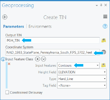
1. 3.Run the tool, and close it after it finishes.
2. 4.In the Contents pane, turn off Contours and Light Gray Canvas basemap, and expand PGH_TIN. The TIN elevation is displayed with elevation heights from high to low.

Change the scene’s surface and coordinate system

The local TIN surface can now replace the surface assigned from the map service.

1. 1.In the Contents pane, right-click TIN Surface Scene > Properties > Elevation Surface > Elevation sources. The dataset PGH_TIN should be the first surface listed as an elevation source using your local drive as the location.
2. 2.Click the red X beside elevation source WorldElevation3D/Terrain3D. This step removes this surface as an elevation source.

1. 3.Click Coordinate Systems. The coordinate system should be the projected coordinate system NAD 1983 State Plane Pennsylvania South FIPS 3702 (US Feet).
2. 4.Click OK, and remove World Light Gray Canvas Base from the Contents pane. Wait for the scene to redraw its features. The scene is now set to local coordinates and TIN as the surface data that could be used offline.

YOUR TURN

TIN units should be in feet or meters, not decimal degrees. Change the scene’s properties for display and elevation units to feet, the default unit for NAD 1983 State Plane Pennsylvania South.

Change the TIN’s symbology

The symbology of a TIN can be changed to better reflect features that the surface model represents. Next, you add the contour and slope symbology renderers.

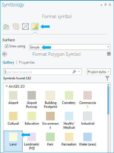
1. 1.In the Contents pane, click PGH_TIN.
2. 2.On the Appearance tab in the Drawing group, click the Symbology arrow and the Slope button .
3. 3.On the Symbology pane, under Draw using, click Simple. Then change the color of the current symbol color to Land.

1. 4.Close the Symbology pane, and zoom to better see the features at all elevations.
2. 5.Use the mouse wheel to view the scene from different angles, including below the scene.
3. 6.Save your project.

 

Tutorial 11-3: Create Z-enabled features

You can create 3D content in different ways, and the corresponding workflows depend on the type of features you create. In addition to creating 3D features from scratch, you can import 3D models and symbolize 2D features as 3D features. You can also specify the source of your z-values when you create new features. ArcGIS Pro’s Current Z control is used to set the 3D elevation source for drawing or obtaining z-values. This option is useful if more than one source is defined for a global or local scene or if you have another source not already included in the map.

In this tutorial, you create a new 3D feature class that is Z-aware. Then you use the Current Z control tool to set the elevation source for populating z-values. The Current Z control has two modes, constant and surface. Constant is used to create 3D features at an absolute height by typing in an exact value—for example, a plane flying at a constant altitude. Surface uses z-values from the active elevation source you choose.

Open the Tutorial 11-3 project

1. 1.Open Tutorial11-3.aprx from Chapter11\Tutorials and save it as Tutorial11-3YourName.aprx. The map opens with 3D Trees Scene, a local scene using World Topographic as the elevation surface whose extent is clipped to a Rivers layer and with a Parks layer draped to the surface.
2. 2.Use the Point State Park bookmark. The map zooms to a large park at the confluence of Pittsburgh’s three rivers.

Create a Z-enabled feature class for park trees

To take advantage of certain 3D editing capabilities, you must ensure an output feature class will have z-values. The Create Feature Class geoprocessing tool lets you determine these settings. Here, you create a new, empty 3D feature class, digitize new features, and populate z-values directly from the map’s surface. If you need to check and see if a layer is Z-enabled, you can verify the data source information listed on the Source page from the Layer Properties dialog box.

1. 1.On the Analysis tab, click the Tools button, and in the Geoprocessing pane, search for and open the Create Feature Class tool.
2. 2.Type or make the selections as shown.

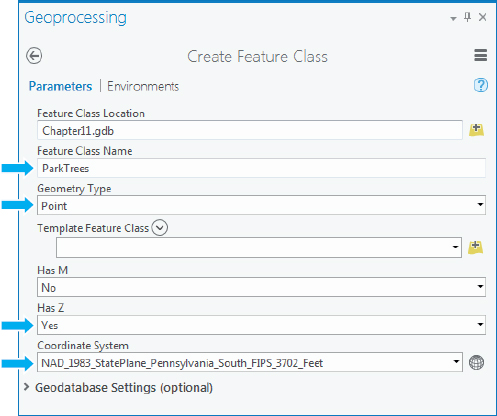
1. 3.Run the tool, and close it after it finishes.
2. 4.Change the ParkTrees symbol to Circle 1 and color to Fir Green.

Digitize trees on surfaces using Z Mode

1. 1.On the Edit tab, in the Elevation group, click the Z control button (Z Mode) . This step will turn the Z control option on.
2. 2.Click the Get Z From View button .
3. 3.Click a point inside the center of Point State Park as shown in the figure to set the z-value (height).

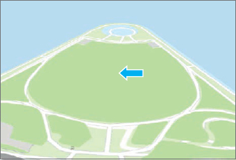
Depending on where you click, the elevation height should be about 723 feet.

1. 4.On the Edit tab in the Features group, click the Create button .
2. 5.In the Create Features pane, select ParkTrees.
3. 6.Click about 10 points to digitize trees on each side of the park. It may take a moment to see each point as you digitize it.
4. 7.Save your edits, and clear the selection.

YOUR TURN

Use the Mt. Washington Park bookmark, set the z-value to various elevations along the large park below Mt. Washington, and digitize about 20 trees at various elevations along the hill. Save your edits, and turn the Z control off.

Use 3D symbols with real-world coordinates

3D tree symbols can be displayed as low resolution, high resolution, or thematic trees. Depending on the number of features and map purpose, you will want to experiment with all three tree types.

1. 1.Zoom to a few trees on one side of Point State Park.
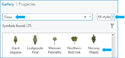
2. 2.In the Contents pane, click the symbol for ParkTrees, click Gallery, click All Styles, type Trees in the search box, and press Enter.
3. 3.Scroll to 3D Vegetation - Realistic, and click Norway Maple.

1. 4.Close the Symbology pane, and zoom in and out. Trees get bigger and smaller depending on the zoom. Next, you will set a fixed height using real-world units and turn shading on for even more realistic trees.
2. 5.In the Contents pane, right-click ParkTrees > Properties > Display, click the box next to Display 3D symbols in real-world units, and click OK.
3. 6.In the Contents pane, right-click 3D Trees Scene > Properties > Illumination, turn on Display shadows in 3D, and click OK. Next, enter an exact height for the park trees.
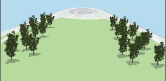
4. 7.In the Contents pane, click the Park Trees symbol > Properties, and type 20 (m) for Size, click Apply, and close the Symbology window.
5. 8.Zoom in and out. Your scene is now populated with realistic-looking trees at a consistent height.

Add realistic preset trees using a table of a tree’s genus (type)

ArcGIS Pro provides preset layers for displaying features in a 3D map. For example, if you have a field with the genus or general type of tree (for example, pine or Pinus), you can display multiple trees by their type.

1. 1.On the Map tab in the Layer group, click Add Preset > Realistic Trees.
2. 2.Navigate to Chapter 11 > Tutorials > Chapter11.gdb, select StreetTrees, and click OK.
3. 3.In the Symbology pane, under Type, click GenusName, and close the Symbology window.
4. 4.Use the Street Trees bookmark. Street trees are draped to various elevations and displayed using the tree genus type.

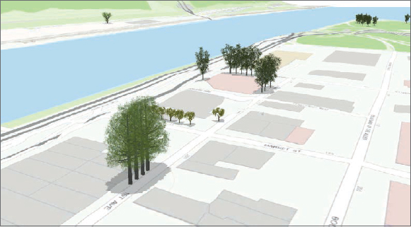
1. 5.Zoom out, and pan the map to see more street trees.
2. 6.Save your project.

 

Tutorial 11-4: Create features and line-of-sight analysis using lidar data

Lidar uses pulsed laser light from aircraft or drones to provide detailed elevation data and classification of land cover that you can use to create 2D surfaces and 3D features. Geographic lidar data is commonly available as lidar aerial survey (LAS) files, the industry standard of the American Society of Photogrammetry and Remote Sensing. In this tutorial, LAS files were provided by Pictometry International Corporation for a study area of Allegheny County, Pennsylvania.

The generation of 3D buildings from lidar LAS datasets requires two surface models, a digital surface model (DSM) and a digital terrain model (DTM) that are then used to create a normalized, nDSM surface, which is the difference between the DSM and DTM surfaces used to calculate building heights. The normalized surface (nDSM) is applied to random points that are created for 2D building footprints. These footprints are used to generate z-values (heights) for each random point. The z-value of the highest point is the building height. The process finishes by creating a statistics table that selects the maximum z-value of the random points that is joined to 2D building footprints, allowing for buildings to be extruded using that value. Lidar data can also be used to determine line-of-sight obstructions between features such as buildings as seen in the last exercise of this tutorial.

Open the Tutorial 11-4 project with a 3D scene

1. 1.Open Tutorial11-4.aprx from the Chapter11\Tutorials folder, and save it as Tutorial11-4YourName.aprx. The project opens with a 3D scene and the building footprints displayed as a 2D layer and a World Light Gray basemap in a local view, with 2D layers for buildings and a lidar delivery area used to clip the basemap. There is no height value in the building attribute table, so buildings can be displayed only as flat 2D polygons for now. Additional layers of observer points used for line-of-sight analysis and a 3D layer for bridges are turned off.
2. 2.Use the 3D View bookmark.

Create an LAS dataset

LAS files have points classified as bare earth, vegetation, buildings, and so on, and are created from original large LAS (American Standard Code for Information Interchange, or ACSII) files, which can then be viewed in 3D or made into raster layers.

An LAS dataset, created from original LAS data, provides fast access to lidar data without the need for data conversion, making it easy to work with LAS files for a specific study area.

1. 1.In the Geoprocessing pane, search for and open the Create LAS Dataset tool.
2. 2.Under Input files, click the browse button, navigate to Chapter 11 > Data > LASFiles, and select the six LAS files.
3. 3.Type or make the changes as shown.

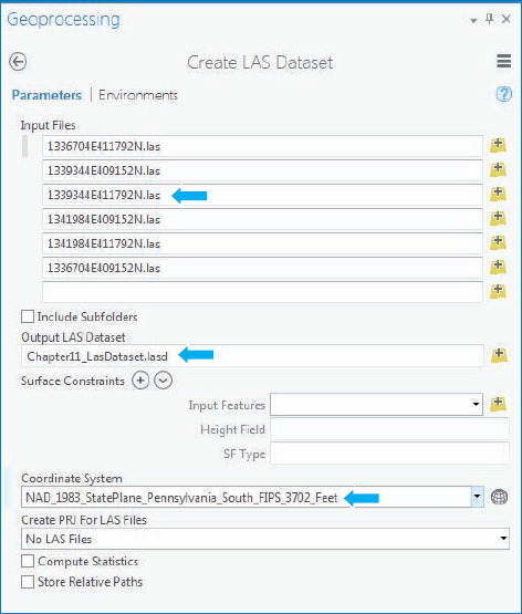
1. 4.Run the tool, and close it after it finishes. The lidar data values are clearly shown as raster points and their values. The LAS dataset can be symbolized using elevations, slope, aspect, and so on. Pittsburgh’s tallest building is the US Steel Building, the triangular building on the right side of the study area.

1. 5.Explore the 3D map from various locations, and then use the 3D View bookmark.

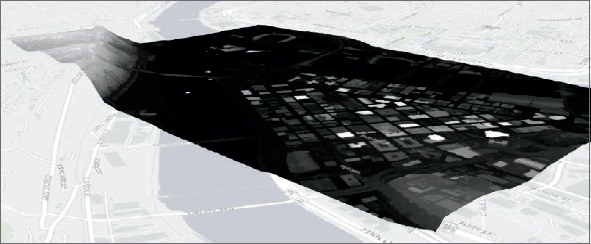
Generate a raster DSM (digital surface model)

DSMs represent the surface of the earth, including buildings, tree canopies, and other obstructions. Before generating the DSM raster, you first filter lidar points to save processing. You will create a DSM using an interpolation type of binning, which is faster for processing, and a maximum cell assignment to find the highest elevation point within each cell.

1. 1.In the Contents pane, right-click Chapter11_LasDataset.lasd > LAS Filters > 1st Points.
2. 2.On the Appearance tab, click the Tools button, and search for and open the LAS Dataset To Raster tool.
3. 3.Type or make selections as shown.

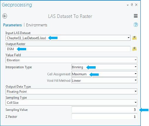
1. 4.Run the tool, and close it after it finishes.
2. 5.Turn the Chapter11_LasDataset.lasd and Bldgs layers off. The values of the DSM show the range of elevations from high to low.

Generate a raster DTM (digital terrain model)

Next, you create the DTM, a bare-earth terrain surface, containing only the topology. In many cases, a DTM is the same as a digital elevation model (DEM). Before creating the raster, you filter the ground features.

1. 1.Turn the DSM layer off.
2. 2.Turn the Chapter11_LasDataset.lasd layer on, and in the Contents pane, right-click Chapter11_LasDataset. lasd > LAS Filters > Ground. This will filter and show only the ground features used to create the DTM.

1. 3.Search for and open the LAS Dataset To Raster tool, and type or make the selections as shown. This raster uses a different interpolation type of triangulation that takes a little longer to process but better interpolates voids found in the earth’s surface.

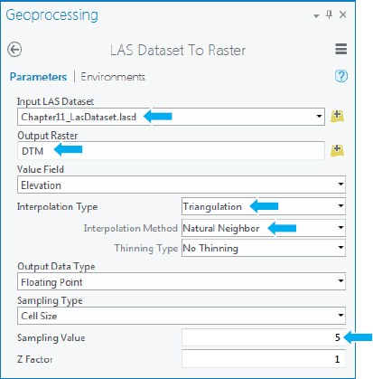
1. 4.Run the tool, and close it after it finishes. A raster surface of the earth’s features is created.

Create a normalized digital surface model (nDSM) raster

An nDSM surface is the difference between the DSM and DTM surfaces that is normalized to the bare-earth surface.

1. 1.In the Geoprocessing pane, search for and open the Minus (3D Analyst Tools) tool.
2. 2.Type or make the selections as shown.

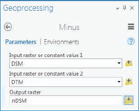
1. 3.Run the tool, and close it after it finishes. You now have a raster surface that can be applied to point features used for buildings to determine their height.

Create random points for buildings

Randomly generated points are created for each building polygon, and then the nDSM raster surface is applied to each random point. The point with the highest z-value will be used as the building height.

1. 1.Turn the Chapter 11_LasDataset layer off and the Bldgs layer on.
2. 2.In the Geoprocessing pane, search for and open the Create Random Points tool.
3. 3.Type or make the selections as shown.

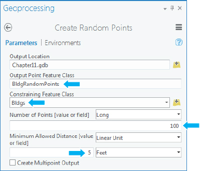
1. 4.Run the tool, and close it after it finishes.

YOUR TURN

Turn all layers off except BldgRandomPoints, and zoom in. Click various random points on each building. Note that the 100 points for the US Steel Building will have a CID value of 521. Every building has a unique CID value that you will use later to join to building footprints.

Add surface information to random points

Here, you assign Z (height) values from the nDSM raster surface to each random point by using the Add Surface Information tool.

1. 1.In the Geoprocessing pane, search for and open the Add Surface Information tool.
2. 2.Type or make the selections as shown.

1. 3.Run the tool, and close it after it finishes.

YOUR TURN

Click on various random points, and note that they now have z-values. The highest value for each building will be used for the building height.

Assign a maximum value (height) to random points

The Summary Statistics tool will calculate the maximum z-value for all buildings using the building’s random points. A text file is created that you will join back to buildings using the CID (unique value for each building) field.

1. 1.In the Geoprocessing pane, search for and open the Summary Statistics tool.
2. 2.Type or make the selections as shown.

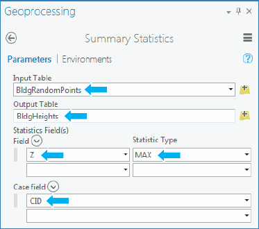
1. 3.Run the tool, and close it after it finishes.

YOUR TURN

Open the BldgHeights table, and sort the MAX_Z field in descending order. Look for CID 521; the tallest building will be the US Steel Building. Close the table.

Join the maximum z-value (height) to building footprints, and display as 3D buildings

1. 1.In the Contents pane, right-click Bldgs > Joins and Relates > Add Join.
2. 2.Join BldgHeights to Bldgs using BLDG_ID for Input Join Field and CID for Output Join Field.
3. 3.Turn the Bldgs layer on, and drag it to 3D Layers in the 3D scene.
4. 4.Turn BldgRandomPoints off, and use the 3D View bookmark.
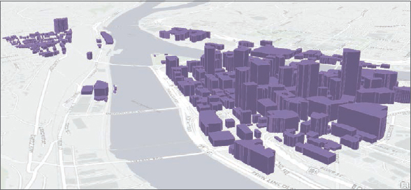
5. 5.On the Appearance tab in the Extrusion group, under Type, click Max Height and [BldgHeights.MAX_Z] as the field. These steps required a lot of processing, but you now have 3D buildings! Notice the residential buildings on the left of the view in the Mount Washington neighborhood as opposed to the taller high-rise buildings in the Central Business District neighborhood.

1. 6.Save your project.

Use lidar to determine bridge elevation heights

You can view and select lidar data points to determine the elevation height to draw bridges. Pittsburgh has more than 750 bridges, but you will use data to find the height and digitize just one.

1. 1.Turn the Bldgs layer off, and use the Fort Pitt Bridge bookmark. Turn the chapter11_LasDataset layer on, and set the LAS Filters to All Points.
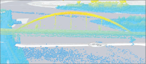
2. 2.On the Map tab, click the Explore button, and click on various lidar points along the bridge to see the z-values (height). Points at the top of the bridge span are approximately 920 feet, while points at the bottom deck range from 770 feet to 800 feet. You will use 775 feet as the elevation to draw the base of the bridge.

1. 3.On the Edit tab in the Elevation group, click the Mode button, and type 775 as the value to set for a constant elevation.

Draw a bridge using a Z elevation

It’s easier to draw the bridge in a 2D map, and you can do so by setting the Z Mode elevation.

1. 1.On the View tab, click Convert.
2. 2.On the Edit tab, in the Elevation group, click the Z Mode button , and type 775 as the constant elevation.
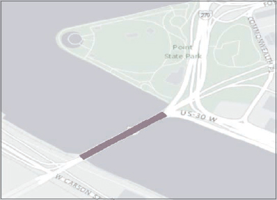
3. 3.Zoom to the bridge as seen in the figure, click the Create button > Bridges layer, and click to digitize the approximate location of the bridge.

1. 4.Save your edits, and close the 2D map to return to the 3D scene. The bottom of the bridge will be at the correct elevation. You can also snap lidar points to create 3D features.
2. 5.Click the Create button > Bridges layer, and click to digitize the bridge span as seen in the figure. Pan and zoom as necessary.

1. 6.Turn the Bridges layer off, and save your project.

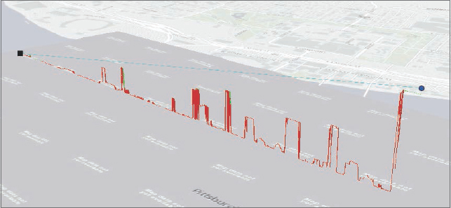
Conduct a line-of-sight analysis

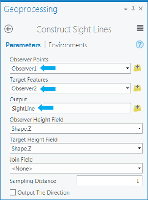
Lidar data can be used to determine line-of-sight obstructions between observer points. This information can be useful for security or development purposes. There are many 3D tools for conducting visibility studies. You will use two, Construct Sight Lines and Line of Sight. In this exercise, you will use two observer points already created, one from the top of the US Steel Building (Observer1) and the other at the fountain at Point State Park (Observer2).

1. 1.Use the Line of Sight View bookmark.
2. 2.On the Analysis tab, click the Tools button > Toolboxes tab, and expand 3D Analyst Tools > Visibility.
3. 3.Click Construct Sight Lines, fill out the form as shown, and run the tool.

A sight line appears in the view between the two observer points.

1. 4.Click the back button, and click Line of Sight.
2. 5.Fill out the form as shown, run it, and then close the tool when it finishes.

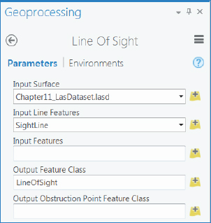
1. 6.Turn the Chapter11_LasDataset layer off to see the features that are visible (green) and not visible (red) between the observer points.

 

Tutorial 11-5: Work with 3D features

This tutorial will explore a few of the many ArcGIS Pro 3D edit and create tools. Some edit functions work only with features that are Z-enabled. If your features are not created as 3D features, you must convert them to 3D before editing using the geoprocessing tools found in the 3D Analyst toolbox. In this tutorial, you will edit building polygons that are already 3D features to create multiple floors in a building and view floors using a range slider and manually edit polygons’ heights using Z constraints.

Open the Tutorial 11-5 project with 3D building polygons

The buildings you edit are the Allegheny County Courthouse and the old county jail, designed by architect H. H. Richardson.

1. 1.Open Tutorial11-5.aprx from the Chapter11\Tutorials folder, and save it as Tutorial11-5YourName.aprx.
2. 2.Use the Courthouse bookmark. The map zooms to the area surrounding the courthouse, on the left, and jail with a 3D feature class of the courthouse, its towers, and the jail.

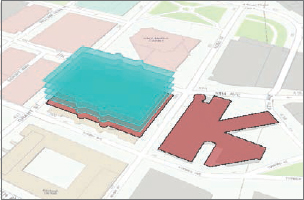
Extrude floors

First, you will create 3D floors for both the courthouse and jail using the Duplicate Vertical tool. You can also use this tool to copy points or lines (for example, furniture or pipes) in a positive or negative direction if your features are above or below ground. You can also select and sketch on each new floor polygon.

1. 1.On the Edit tab in the Tools gallery, click the Duplicate Vertical button .
2. 2.Click the Allegheny County Courthouse polygon, and make the changes as shown.

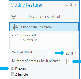
1. 3.Click Duplicate. There are a total of five floors, and the Preview box will show the building floors as they are extruded.

1. 4.Clear the selected features, and save your edits.

YOUR TURN

Use the Duplicate Vertical tool to extrude the floors of the old jail (building on the right) an offset of 20 feet, and use 3 for the number of times to duplicate. Clear your selections, save your edits, and close the Modify Features pane.

Use a range slider to view building floors

Setting range values offers a way to visualize certain floors in a building. This visualization method is especially useful if a floor contains detailed information or if a building has many floors. You can use this tool to visualize numeric values in an attribute table, including property values for parcels, crimes in neighborhoods, and so on.

1. 1.Use the Building Floors bookmark.
2. 2.Open the Courthouse3D attribute table, and sort by Name.
3. 3.Select each floor of the Courthouse, and in the corresponding FloorNumber field, type 1 for the first (lowest) floor, 2 for the second floor, 3 for the third floor, and so on. Repeat for the jail floors.
4. 4.Clear your selection, save your edits, and close the table.
5. 5.In the Contents pane, right-click Courthouse3D > Properties > Range >Add Range, click FloorNumber, click Add, and click OK.
6. 6.Drag the slider to 3, and notice floors 1 and 2 disappear from view. You can use range sliders in 3D animations, and you can modify range properties on the Map Range ribbon.

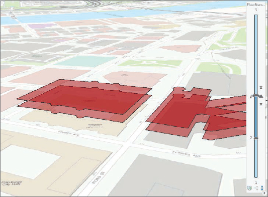
1. 7.Drag the slider to 1 to view all floors.
2. 8.On the Range tab in the Active Range group, click <None> for value. This will turn off the range slider.

Edit a building’s height using dynamic constraints and the attribute table

Buildings are sometimes composed of multiple polygons at different heights. If these heights are not already derived from lidar data, you can use interactive handles to adjust the building height dynamically using a Z constraint or by typing building height using attributes.

1. 1.In the Contents pane, turn Courthouse3D off and Courthouse3DTowers on.
2. 2.On the Edit tab, click the Z Mode button to turn it off.
3. 3.Click the Modify button, and in the Modify Features pane under Alignment, click Scale, and then click the large tower on Grant Street.

The dynamic constraint icon will appear on the tower polygon. If your icon does not appear, you can turn on “Show dynamic constraints in the map” by clicking Project, then Options, and then Editing. You can adjust the map if necessary to better see the tower and constraint icon.

1. 4.Click the green (Z) constraint to scale the tower in the Z direction to the height of the rectangular part of the tower. If you have lidar data, snap to those points.
2. 5.Click to finish the tower.

1. 6.Save your edits.

YOUR TURN

Drag the smaller towers to the eastern side of the building. An alternative to dragging features is to simply type the building heights in the corresponding attribute table. Open the Courthouse3DTowers attribute table, and type 150 for the smaller tower’s height. Clear your selected features, and save your edits and your project.

 

Tutorial 11-6: Use procedural rules and multipatch models

A CityEngine rule package (.rpk) is a compressed file that contains a compiled rule and all the assets (textures and/or 3D models) that the rule logic uses for creating 3D content. You can use these packages in ArcGIS Pro as a procedural symbol that constructs and draws the procedural features on the fly from the source data. Another method creates 3D models and stores them as a feature class called a multipatch, whose features are a collection of “patches” that represent the boundary of a 3D object. A multipatch stores color, texture, transparency, and geometric data in its features.

Here, you will apply a predefined rule package to Pittsburgh’s tallest office building, the US Steel Building. You will also view multipatch features whose building facades were created in CityEngine using actual building facades. These features can take a long time to render, so it’s recommended to use a high-end graphics card and follow the hardware requirements.

Open the Tutorial 11-6 project with a building footprint

When you apply procedural rules, features must be displayed as layers in a 3D scene. The feature class polygon itself does not have to include z-values but must be in a 3D scene and viewed as 2D layers.

1. 1.Open Tutorial11-6.aprx from the Chapter11\Tutorials folder, and save it as Tutorial11-6YourName.aprx. The project opens with a 3D scene—US Steel Building—and one 2D building polygon footprint.
2. 2.Use the US Steel Building bookmark.

Apply building rules using stacked blocks

You can easily apply a procedural rule to a building for a stacked block or more realistic high-rise or office building.

1. 1.In the Contents pane, click the red symbol for the US Steel Building.
2. 2.In the Symbology pane, click Gallery > All styles, and in the search box, type Procedural, and press Enter. Procedural rules will update with new software releases and can be downloaded and added from CityEngine or Esri’s Living Atlas of the World.
3. 3.Click the Stacked Blocks procedural symbol.
4. 4.In the Symbology pane, click Properties and the Layers button .
5. 5.Under Units, click Feet; under Total Height, click the Container button on the right of the current height; click the [Height] field; and click OK. This step sets the building height to a height field in which building heights are already entered.
6. 6.Fill out the form as shown, click Apply, and drag the USSteelBldg layer to 3D Layers.

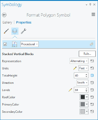
The building will now be “wrapped” showing the number of floors.

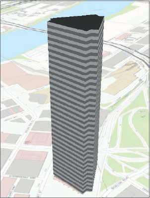
Apply an international building rule

The unit for international buildings is meters, so you will type the height instead of using the building height field, which is in feet.

1. 1.In the Symbology pane, click Gallery, click the International Building procedural symbol, click Properties, and then click the Layers button.
2. 2.Fill out the form as follows, and click Apply.

Although the result does not look exactly like the actual US Steel Tower, it is more realistic than a wrapped, level building.

1. 3.Close the Symbology pane.

View multipatch models of buildings and street furniture

Smithfield Street is a study area in downtown Pittsburgh using multipatch layers of exported SketchUp Collada (.dae) files with realistic building images and street furniture. You will turn on these layers to explore multipatch models.

1. 1.Close the US Steel Building scene, and open the Smithfield Street scene.
2. 2.Use the Smithfield Street bookmark. Wait while the buildings display the building facades with textures.
3. 3.Turn on Smithfield Furniture, and wait for the view to render. This layer of detailed features such as planters, garbage and recycling cans, and newsstands might take a while to render, depending on your graphics card.

YOUR TURN

Turn off the Smithfield Furniture layer, and turn on the Smithfield Textured 2 layer. View the scene from various locations, including the Smithfield Street Bridge. Turn on the Smithfield Buildings layer, and on the Appearance tab, in the Effects group, change the transparency to 50 percent. Save your project.

 

Tutorial 11-7: Create an animation

Animations are created by capturing an ordered set of viewpoints as keyframes and managing how the camera transitions between them. In this tutorial, you will take advantage of the bookmarks already in the scene to build a fly-through animation of downtown Pittsburgh. You will then improve the flight path and flight speed by manually inserting more keyframes and adjusting their timing.

Open the Tutorial 11-7 project, and explore bookmarks

1. 1.Open Tutorial11-7.aprx from the Chapter11\Tutorials folder, and save it as Tutorial11-7YourName.aprx.
2. 2.On the Map tab, click Bookmarks > Manage Bookmarks, and double-click each bookmark in order, from Frame1 through Frame8. You will use these bookmarks to create the animation.
3. 3.Double-click the Frame1 bookmark. This bookmark will be the first camera location of your animation.

Add an animation to the project, and create keyframes

Adding animation to a project enables the animation functions. As soon as you add an animation, you begin making keyframes manually. You can also import keyframes into an animation on the Animation tab in the Create group by using the Import function.

1. 1.On the View tab in the Animation group, click the Add button . The Animation ribbon opens, and an Animation Timeline pane appears at the bottom of the screen. You are ready to make your first keyframe using bookmarks.
2. 2.In the Animation Timeline pane, click Create first keyframe. A thumbnail image of the starting location (Frame1 bookmark and the first keyframe) will appear.

1. 3.On the Bookmarks pane, double-click Frame2, and in the Animation Timeline, click the Append Next Keyframe button . This step adds the next keyframe to the animation.
2. 4.Repeat step 3 for each of the remaining bookmarks, Frame3 through Frame8.
3. 5.Close the Bookmarks pane. This step adds all keyframes to the animation.

Play an animation, and change the duration

The keyframes have durations of three seconds between each frame for a total duration of 21 seconds. You can play the animation for this duration or extend the playback time.

1. 1.On the Animation tab in the Playback group, click the Play button . On the Animation Timeline tab, the spacebar is a keyboard shortcut for Play/Pause.
2. 2.On the Animation tab in the Duration box, type 00:30.000.
3. 3.Play the animation from the beginning. The animation will now play for 30 seconds.

Create a pause

Holding a keyframe will pause the animation at the selected frame. Here, you will add a hold to create a slight pause between frames 5 and 6 along the Smithfield Street Bridge.

1. 1.On the Animation Timeline, double-click keyframe 5, and click the Hold button .
2. 2.Play the animation from the beginning, and observe the slight pause between frames 5 and 6.

Add and delete keyframes

Keyframes can be moved to adjust the speed of animations, and frames can be inserted in between keyframes using different camera locations. Here, you will add a new keyframe and manually adjust the camera.

1. 1.On the Animation Timeline, drag the Time Indicator (red vertical bar) to approximately 21 seconds (about halfway between frames 6 and 7). Moving the Time Indicator “scrubs” through time, and the location where you move it is where you will adjust the camera and insert a new keyframe.
2. 2.Using the mouse wheel or keyboard keys, adjust the view to a slightly lower focal point.
3. 3.On the Animation timeline, click the Insert button . Because no keyframe existed at 21 seconds, when you click update, it will insert a new keyframe to capture the camera change and add a new keyframe using the current camera location.
4. 4.Play the animation from the beginning.

View an animation’s path, and manually edit a keyframe’s properties

When adjusting animations, it’s useful to see the camera’s path and keyframes so that you can move to a keyframe and adjust its properties, such as Z elevation (camera location).

1. 1.On the Animation Timeline, double-click frame1, and zoom out.
2. 2.On the Animation tab in the Display group, click the Path button . This step turns the camera path and keyframes on to better see how the animation plays. Keyframe 2 is a little too high, so you will edit its properties to lower the keyframe.
3. 3.On the Animation Timeline in the Keyframe Gallery, double-click keyframe 2.
4. 4.On the Animation tab in the Edit group, click the Properties button , expand Camera, and type 1000 for the z-value.
5. 5.Close the Animation Properties pane, and click the Path button to turn off the path.
6. 6.Play the animation from the beginning. Notice that the camera is lower at keyframe 2.

Create a movie from the animation

Now that you have created an interesting animation, it’s time to share the animation with others. To share the animation, you will export a movie to a file. You have several options, including exporting your movie directly to YouTube, Vine, Vimeo, and so on, or as a draft animation. You can change the file location and movie resolution, type, size, and so on in the File Export and Advanced Movie settings.

1. 1.On the Animation tab in the Export group, click the Export Movie button .
2. 2.In the Export Movie pane in the Movie Export Presets group, click the Draft button. This step will create a smaller file. The resulting quality of the file isn’t high, but it is much faster to produce.
3. 3.Under file name, click the Browse button, navigate to Chapter11\Tutorials, and type Chapter11Animation3D as the movie name. MPEG4 (.mp4) is the default type.
4. 4.In the Export Movie pane, click Export. Wait while the movie is created. If you use other settings with higher resolutions or a larger size, the movie can take a long time to render. You can save the media format as separate .jpg files that you could later stitch together using another animation software application.
5. 5.In Windows Explorer, navigate to Chapter 11\Tutorials, and double-click Chapter11Animation3D.mp4 to play the movie.
6. 6.Save your project.

Assignments

This chapter has two assignments to complete that you can download from this book’s resource web page, esri.com/gist1arcgispro:

• Assignment 11-1: Prepare 3D building and topography features for a 3D study.
• Assignment 11-2: Create a realistic 3D scene for a campus study.