Chapter 3
Using Advanced Functions

Now that you have completed the initial design, you are ready to take steps to make it even better. The Autodesk^® Roadway Design for InfraWorks^® 360 vertical application provides tools for optimizing and analyzing your design as well as a tool for pushing it into the detailed design stages that are taken care of by Autodesk^® AutoCAD^® Civil 3D^® software. By using these tools, you are moving your design from an early conceptual version toward a well-engineered version that is poised for detailed design.

---

In this chapter, you'll learn to

• Balance earthwork and minimize cost using Profile Optimization
• Analyze roadways and intersections for sight distance issues
• Generate Civil 3D drawings of your road design

---

Using Profile Optimization

When you first draw a road in InfraWorks 360 using the Roadway Design for InfraWorks 360 tools, the software makes its best guess at balancing “smooth” road geometry with a close match to the existing terrain. As a result, you are given an initial design profile that is then modified and adjusted repeatedly as the design progresses. This profile is the “backbone” of the road model and is the single greatest influence on the earthwork quantities that will be produced based on your road design.

Questions about cut and fill quantities will be among the first questions posed about your design because excavation is such an expensive part of construction. As a designer, you will be called upon to minimize cut and fill quantities and to report your results in detail. Typically, adjusting the profile to achieve the best earthwork results is an iterative process— adjust it a little higher here, a little lower there, and run the volume analysis. Then repeat as many times as necessary until earthwork results appear to be the best they can be. As you might guess, or as you may have experienced, this process is time-consuming and repetitive.

What if you could click a magic button that would perform all of these iterations for you? What if the computing power needed to perform such an optimization was readily available? Well, through the cloud via InfraWorks 360 technology and a function called Profile Optimization, this is all a reality. Not only will Profile Optimization balance your road earthwork, it will also provide a detailed cost analysis that you can use to assess the overall cost of the road, not just earthworks.

Using the Profile Optimization Panel

To begin a profile optimization, you will need to open the Profile Optimization panel. This is done by clicking the Analysis icon of the Roadway Design toolbar and then clicking Profile Optimization on the Analysis toolbar (see Figure 3.1).

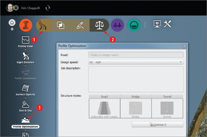
Figure 3.1 The Profile Optimization panel can be opened by clicking the icons in the order shown.

In the top portion of the Profile Optimization dialog are some general settings (see Figure 3.1). They are described as follows:

1. Road This is the name of the road as you would see it in the Summary section of the Road asset card.
2. Design Speed The Profile Optimization function is going to redesign your profile. This setting will establish the design constraints for things such as vertical curve length, stopping sight distance, and so on.
3. Job Description When you submit your optimization, it will be sent as an optimization job to InfraWorks 360 cloud services, and you will be able to check on it using the Job Monitor (covered a little later in this chapter). Job Description will help you distinguish between multiple jobs if you've submitted multiple optimizations.
4. Structure Styles When the optimization encounters things such as ravines and mountains, it will determine the most cost-effective course to take. Sometimes that will require tunneling through a mountain or placing a bridge across a ravine. This section is your opportunity to assign styles to those structures should they be needed.

Once you have selected a road for optimization, you will be given access to the Advanced Settings section of the Profile Optimization panel. The Advanced Settings section is divided into several subsections, with each containing a set of functions and options. A summary of each subsection and the items within it follows:

1. Profile Constraints This section gives you the opportunity to establish some ground rules about how you want InfraWorks 360 to redesign your profile (see Figure 3.2).
   1. Maximum Grade This establishes the steepest grade allowable on the tangent sections of the profile. The initial value is set when you provide a value for Design Speed; however, you can change it after doing so.
   2. Minimum PVI Spacing The optimization process will create additional PVIs in your profile. This value establishes a minimum distance between them. Increasing this value will result in a “smoother” profile with fewer PVIs.
   3. Required Drainage Grade This is the minimum grade allowed for the tangent sections of the profile. Try to set this at the minimum value possible, because if it is too high, it may prevent the optimization from finding a solution.
   4. PVI Frequency This will affect the “smoothness” as well, but it is a bit different from Minimum PVI Spacing. This is a more general setting that will affect the distribution of PVIs across the entire profile.
   5. Anchored PVIs In addition to the profile constraints just mentioned, there may be other considerations that require the profile to maintain certain elevations in a given area. This is your opportunity to “lock down” those areas by choosing PVIs that are to be preserved during the optimization. This means that during the optimization process they will not be deleted, and they will hold their current station and elevation. For example, you might lock down PVIs near an existing road intersection or in front of a building where you know that the current road elevations must be preserved. The first and last PVIs are always anchored and cannot be changed.

      You can click Profile View to open the Profile View panel while you are configuring Anchored PVIs. Also, if you double-click a PVI in the list, the model will zoom to that PVI, and it will be highlighted in red in the Profile View panel.

2. Quantities Options In this section, you can add borrow pits and waste pits to your design (see Figure 3.3). Each one is assigned Station, Access Distance, and Capacity values. These locations will be considered in the mass haul aspects of optimizing the profile.
3. Construction Rules In this section, you specify the thresholds for the creation of bridges and tunnels (see Figure 3.4). For bridges, this is a maximum fill height, and for tunnels, this is a maximum cut depth.
4. Construction & Earthwork Cost In this section, you assign cost values for earthwork and construction. Earthwork costs include items such as excavation, borrow, waste, and so on; construction costs include items for pavement, bridges, tunnels, signing, and others. To access these settings, you click the link in the Profile Optimization dialog to open the Construction & Earthwork Costs Settings dialog (see Figure 3.5).

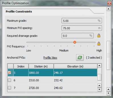
Figure 3.2 The Profile Constraints section of the Profile Optimization panel

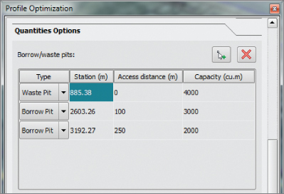
Figure 3.3 The Quantities Options section of the Profile Optimization panel

---

What Is Mass Haul?

Without getting too technical, mass haul is the concept of tracking the excavation, movement, and placement of earth during the process of constructing a road. By analyzing mass haul, these activities can be minimized, thereby minimizing the cost to construct the road.

---

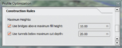
Figure 3.4 The Construction Rules section of the Profile Optimization panel

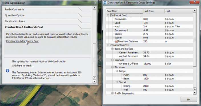
Figure 3.5 To open the Construction & Earthwork Costs Settings dialog, click the link in the Profile Optimization dialog.

Once you have addressed everything you need in the Profile Optimization panel, click Optimize It (see Figure 3.6). When you do, InfraWorks 360 will package all of the information it needs and submit it to the cloud for analysis.

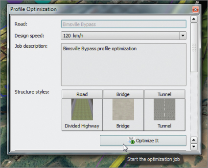
Figure 3.6 Launching a profile optimization

Exercise 3.1: Optimize Your Profile

In this exercise, you will optimize the profile for a section of the Bimsville Bypass road.

---

Attention: This Exercise Requires Cloud Credits

You are going to perform a function during this exercise that requires cloud credits. Please check with the person in your company or organization who is responsible for issuing cloud credits to ensure that you are permitted to use them for this purpose.

If you are unfamiliar with the concept of cloud credits, you can think of them as Autodesk 360 currency. Your company will buy cloud credits that you can use to perform functions such as the profile optimization discussed here. They cost money, so be careful with how you use them and get permission before you do.

If you do not have access to cloud credits, pay attention to the exercise instructions, and you will be notified about which steps you cannot perform.

---

Go to the book's web page at www.sybex.com/go/roadwaydesignessentials2e and download the files for Chapter 3. Using the instructions in the Introduction, unzip the files to the correct location on your hard drive.

1. If it is not already open, launch InfraWorks 360. If you have a model open, click the Switch To Home icon to return to InfraWorks 360 Home.
   
2. On InfraWorks 360 Home, click Open. Browse to C:\InfraWorks Roadway Essentials\Chapter 03\, and select Ch03 Bimsville Roads.sqlite. Click Open.
3. On the Utility Bar at the top right of your screen, click the Proposals drop-down list and select Ex_3_1_and_3_2.
4. Restore the bookmark named Bimsville Bypass.
5. Click the Roadway icon to expand the Roadway toolbar.
   
6. On the Roadway toolbar, click the Analysis icon to display the Analysis toolbar along the left side of the InfraWorks window.
   
7. On the Analysis toolbar, click Profile Optimization.

   The Profile Optimization panel will open.
   

8. Click the Bimsville Bypass road.

   When you select the road, the Road property on the Profile Optimization panel will automatically say Bimsville Bypass, and the Optimize It button will activate.

9. Click Advanced Settings and then click Profile Constraints.
10. Next to Anchored PVIs, click Profile View.

    The section of road that you are viewing has all of the PVIs removed, except for the first and last (see Figure 3.7). This was done so that the effects of the optimization are quite apparent when the optimization is complete.

11. In the Profile Constraints section, do the following:
    • For Minimum PVI Spacing, enter 500 (150).
    • For Required Drainage Grade, click the lock icon to unlock the value. Enter 0.5 (for both Imperial and metric users).
    • For PVI Frequency, click the lock icon to unlock the value and move the slider to the Medium position.
12. Click Optimize It.

    If you are not logged in or do not have cloud credits available, you will not be able to perform this step or the next step.

    If you are successful, a dialog will open indicating that the optimization is being processed.

    When the data has been successfully sent for optimization, the Job Monitor panel will open, and your recently submitted job should be displayed with a status of In Progress, as indicated by the double blue arrows.

13. Close the Profile Optimization panel, Road asset card, Profile View panel, and Job Monitor panel.

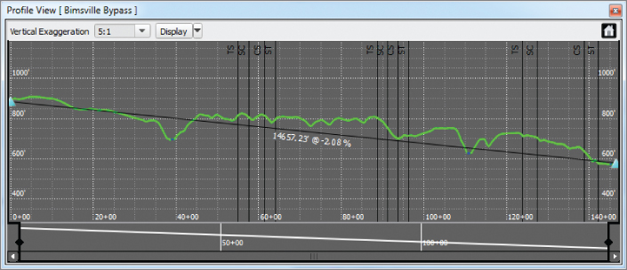
Figure 3.7 The initial profile, prior to optimization

Getting Your Optimization Results

Once you have submitted a job for optimization, the Job Monitor panel will open, showing you all of the optimization jobs that you have submitted to InfraWorks 360 cloud services. If you close this panel, you can open it by clicking Job Monitor on the Analysis toolbar (see Figure 3.8).

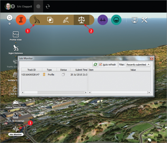
Figure 3.8 The Job Monitor panel (to open it, click the icons in the order shown)

When your optimization is complete, the Status column will display a green check mark. Also, when your optimization is complete, you will see icons in the Report and Result columns. If you click the icon in the Report column, you will download and open a PDF showing information about your optimization, including the new profile design, cost of construction, earthworks data, and cross-section views (see Figure 3.9).

---

You will also receive an email informing you that optimization is complete.

---

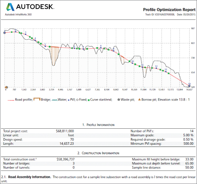
Figure 3.9 The first section of a Profile Optimization report

If you click the Results icon, you will download an IMX file and then be prompted to import the results into your InfraWorks model as a new proposal (see Figure 3.10). If you are satisfied with the results, you can use the Merge Proposals function on the Proposals panel to replace your old road design with the optimized one.

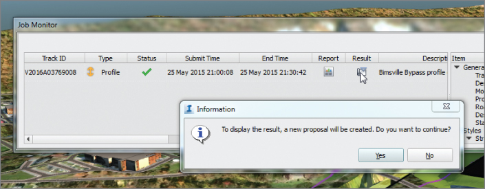
Figure 3.10 Importing optimization results into an InfraWorks model

Exercise 3.2: Get Your Optimization Results

In this exercise, you will view the results of the optimization that you performed in Exercise 3.1. You will also update your model by creating a proposal from the optimized road and merging it with your current proposal.

If you are continuing from the previous exercise, you can skip to step 3. Otherwise, if you haven't already done so, go to the book's web page at www.sybex.com/go/roadwaydesignessentials2e and download the files for Chapter 3. Following the instructions in the Introduction, unzip the files to the correct location on your hard drive.

1. If it is not already open, launch InfraWorks 360.
   
2. On InfraWorks 360 Home, click Open. Browse to C:\InfraWorks Roadway Essentials\Chapter 03\. Click Ch03 Bimsville Roads.sqlite and click Open.
3. On the Utility Bar at the top right of your screen, click the Proposals drop-down list and select Ex_3_1_and_3_2.
4. Restore the bookmark named Bimsville Bypass.
5. Click the Roadway icon to expand the Roadway toolbar.
   
6. On the Roadway toolbar, click the Review icon to display the Review toolbar along the left side of the InfraWorks window.
   
7. On the Analysis toolbar, click Job Monitor.
   

   The Job Monitor panel will open. If you completed Exercise 3.1 and enough time has passed (about 30 minutes), then you should see an entry with a description of “Bimsville Bypass profile optimization” and a green check mark in the Status column. If not, further instructions will follow.

8. Click the icon in the Report column. If you do not have access to this icon, you can open Bimsville Bypass.pdf located at C:\InfraWorks Roadway Essentials\Chapter 03\Optimization Results\.

   A PDF of the report will open. Notice that the new profile has 14 total PVIs. You started with 2.

9. Study the report, and close it when you are done.
10. In the Job Monitor panel, click the icon in the Result column. If you have not completed Exercise 3.1 or if your results are not available, set Ex_3_1_and_3_2_End as the current proposal. Read through the next steps, but don't perform any of the actions until you get to step 19.

    A dialog will open informing you that a new proposal will be created if you continue.

11. Click Yes to create a new proposal.
12. In the Add New Proposal dialog, enter Optimized_Bimsville_Bypass in the Name field. Click OK.

    Optimized_Bimsville_Bypass will now be your current proposal.

13. Change the current proposal back to Ex_3_1_and_3_2.
    
14. Click the InfraWorks Home icon.
    
15. Click the InfraWorks Manage icon.
    
16. On the Manage toolbar, click Proposals.

    The Proposals panel will open.

17. In the Proposals panel, click Merge Proposals.
    
18. In the Merge Proposals dialog, click Optimized_Bimsville_Bypass and then click OK.

    After a pause, the model will update and the Bimsville Bypass road will be replaced with the new design.

19. Click Profile View on the Analyze toolbar of the Roadway Design tools.
    
20. Click the newly imported road to view its profile in the Profile View panel.

    This version of the profile has many more PVIs.

21. Study the profile and take note of how the optimization process redesigned it (see Figure 3.11).

    Compare this profile with Figure 3.7. Notice how the slopes are all between 0.5 percent and 5 percent. These were the values you provided for Required Drainage Grade and Maximum Grade. Notice also that there is always at least 500 feet (150 meters) between PVIs because of the Minimum PVI Spacing value you provided.

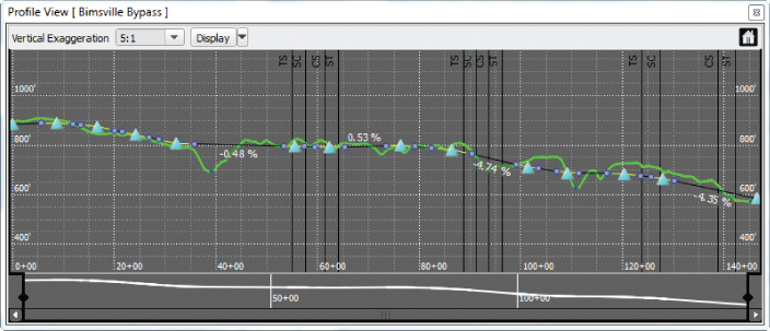
Figure 3.11 An optimized profile

Analyzing Sight Distance

Of course, one of the most important aspects of road design is driver safety, and one of the best ways to keep drivers safe is to give them good visibility. For that reason, a sight distance analysis is an important part of every road design. In the past, sight distance analyses have been time-consuming and expensive. But now you have an engineering-accurate 3D model and the power of InfraWorks technology. It has become almost too easy.

To perform a sight distance analysis, you will need the Sight Distance panel, which you open by clicking Sight Distance on the Analysis toolbar (see Figure 3.12). You can perform a sight distance analysis for two scenarios: a roadway and an intersection.

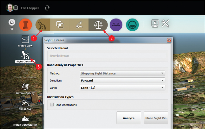
Figure 3.12 Open the Sight Distance panel by clicking the icons in the order shown.

Analyzing a Roadway for Sight Distance

If you choose a road for sight distance analysis, you will be presented with the following options on the Sight Distance panel (see Figure 3.13):

1. Road Analysis Properties This section is used for setting up the configuration of the analysis.
   1. Method The method can be Stopping Sight Distance or Passing Sight Distance. For roads that have multiple lanes in either travel direction, only the Stopping Sight Distance method is available.
   2. Direction The direction is determined by the way you drew the road when you created it. If you drew it south to north, then the northbound lanes are Forward, and the southbound lanes are Backward.
   3. Lane For multilane roads, choose the lane you want to analyze. This works outward from the centerline; for example, if there were two northbound lanes, the inside lane would be Lane - (1), and the outside lane would be Lane - (2).
2. Obstruction Types If you want the sight distance analysis to consider 3D objects in the model, you can check the box next to Road Decorations.
3. Visual Options The analysis shows results along the road using a number of colored zones and envelopes (see Figure 3.14). In this section, you can choose which indicators are visible and which are not.
   1. Road: Sight Zones Sight zones are colored lines that appear along the lane you've selected. They indicate Sight Clear areas (light greenish-blue) or Sight Failure areas (yellow).
   2. Road: Accident Zones Accident zones are areas that are especially prone to accidents because of poor sight distance. These areas are shown as dark greenish-blue lines within the lane you're analyzing.
   3. Road: Sight Envelopes Sight envelopes are light blue areas where obstructions are analyzed and, if they're found, are highlighted in orange.
   You can also place a sight pin on your analysis: a single point from which you assess sight distance. There are visual indicators for sight pins too (see Figure 3.15).
   1. Sight Pin: Sight Regions This is the region that is analyzed for obstructions. It is shown in several colors, with orange representing obstructions.
   2. Sight Pin: Sight Lines If no obstruction is present, a sight line is a straight line from the sight pin to the end of the sight distance. If there is an obstruction, additional lines will appear indicating the first and last lines along which the obstruction is encountered.
   3. Sight Pin: Distance Line This is a black line with an arrowhead at the end that follows the path of the lane. The tip of the arrow indicates the required sight distance from the sight pin.

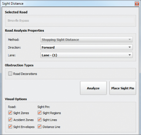
Figure 3.13 The Sight Distance panel for roads

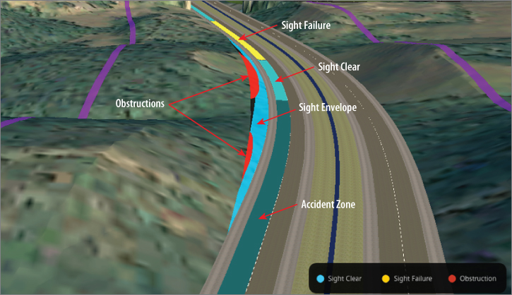
Figure 3.14 Sight distance analysis indicators for roads

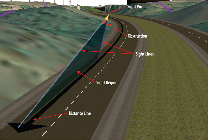
Figure 3.15 Sight distance analysis indicators for sight pins

---

What Happened to Driving Side?

If you're really paying attention and you're familiar with earlier versions of the InfraWorks 360 program, you may wonder where the Driving Side option is in the Sight Distance dialog. That option has been moved to the Model Properties dialog under Road Design Standards.

---

Exercise 3.3: Analyze a Road's Sight Distance

In this exercise, you will perform a sight distance analysis for a section of the Bimsville Bypass.

If you are continuing from the previous exercise, you can skip to step 3. Otherwise, if you haven't already done so, go to the book's web page at www.sybex.com/go/roadwaydesignessentials2e and download the files for Chapter 3. Using the instructions in the Introduction, unzip the files to the correct location on your hard drive.

1. If it is not already open, launch the InfraWorks 360 program.
   
2. On InfraWorks 360 Home, click Open. Browse to C:\InfraWorks Roadway Essentials\Chapter 03\. Click Ch03 Bimsville Roads.sqlite and click Open.
3. On the Utility Bar at the top right of your screen, click the Proposals drop-down list and select Ex_3_3_and_3_4.
4. Restore the bookmark named Road SDA.
5. Click the Roadway Design icon to expand the Roadway Design toolbar.
   
6. On the Roadway Design toolbar, click the Analysis icon to open the Analysis toolbar along the left side of the InfraWorks window.
   
7. On the Analysis toolbar, click Sight Distance.

   The Sight Distance panel will open.
   

8. Click the Bimsville Bypass road.

   The functions on the Sight Distance panel will activate. Notice that the only available choice for Method is Stopping Sight Distance. Passing Sight Distance is not available, because this road has multiple lanes.

9. On the Sight Distance panel, do the following:
   • For Direction, select Backward.
   • For Lane, select Lane - (2).
   • Click Analyze.

   After a pause, indicators from the analysis should appear in the model.

10. Under Visual Options, check all of the options under Road.

    You should see various colored areas representing different key findings for the analysis.

11. Hover your cursor in the yellow area.

    Note the tooltips that indicate the Sight Failure and Accident Zone areas, as shown in Figure 3.16. The failure is caused by the embankment (highlighted in orange) that is obstructing a driver's view of the required sight distance.

12. In the Sight Distance panel, click Place Sight Pin. Click a point within the yellow Sight Failure area.
13. In the Sight Distance panel, within the Visual Options section, uncheck all boxes under Road and verify that all boxes under Sight Pin are checked.
14. Zoom in and study the graphics representing the sight pin analysis, as shown in Figure 3.17.

    You should see two sight lines: one projecting to the end of the sight distance (the end of the black arrow) and the other passing through the first point obstructed by the embankment. The zone between them represents the sight region where the obstruction has an effect. You should also see the embankment highlighted in orange, indicating the source of the obstruction.

    Because there was no change to the model, there is no Ex_3_3_and_3_4_End proposal for this exercise.

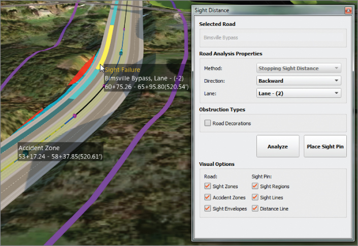
Figure 3.16 Sight Failure and Accident Zone areas revealed by a sight distance analysis

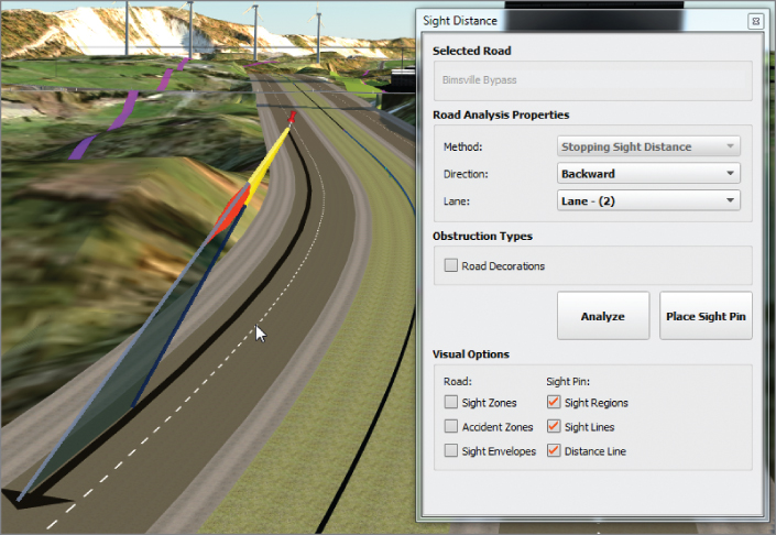
Figure 3.17 Analyzing sight distance using a sight pin

Analyzing an Intersection for Sight Distance

An intersection is another key location where sight distance is especially important. The Sight Distance panel handles intersections a bit differently, and as a result, different options are presented when you select an intersection (see Figure 3.18).

1. Intersection Analysis Properties In this section, you configure the analysis.
   1. Approach For four-way intersections, you can choose which approach road you are analyzing and in which direction. For three-way intersections, this is always the “stem” of the T.
   2. Traffic Control Here you can choose from No Control, Stop Control, and Yield Control. Each option has different sight distance requirements. No Control means that traffic will travel right through the intersection without regard for the other intersecting roads. Stop Control and Yield Control are self-explanatory.
   3. Maneuver Choose from Left Turn or Right Turn.
2. Obstruction Types Use this section to choose whether you want road decorations (signs, hydrants, and so on) to be analyzed.
3. Visual Options For now, this section has only the Sight Triangles option, which is the only visual indicator available. Perhaps there will be more options here in the future.

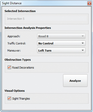
Figure 3.18 The Sight Distance panel for an intersection

When you run the analysis, you will see the results as visual indicators (see Figure 3.19). Sight triangles indicate the required visibility as a vehicle approaches the intersection. If the triangle is light blue, the approach is clear; if it is yellow, the approach is obstructed. An arrow showing the path of the vehicle will be colored yellow if there are any sight distance issues and will be colored light blue if it is all clear. Obstructions will be highlighted in orange.

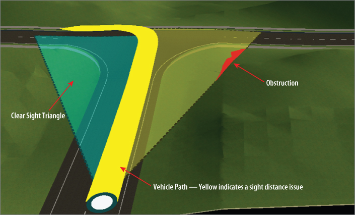
Figure 3.19 An intersection sight distance analysis

Exercise 3.4: Analyze an Intersection's Sight Distance

In this exercise, you will perform a sight distance analysis for an intersection within the industrial park. You will correct a sight distance issue by performing some simple grading.

If you are continuing from the previous exercise, you can skip to step 3. Otherwise, if you haven't already done so, go to the book's web page at www.sybex.com/go/roadwaydesignessentials2e and download the files for Chapter 3. Using the instructions in the Introduction, unzip the files to the correct location on your hard drive.

1. If it is not already open, launch the InfraWorks 360 program.
   
2. On InfraWorks 360 Home, click Open. Browse to C:\InfraWorks Roadway Essentials\Chapter 03\. Click Ch03 Bimsville Roads.sqlite and click Open.
3. If it has not already been done in the previous exercise, on the Utility Bar at the top right of your screen, click the Proposals drop-down list and select Ex_3_3_and_3_4.
4. Restore the bookmark named Intersection SDA.
5. If the Sight Distance panel is already open, you can skip to step 8. Otherwise, click the Roadway Design icon to expand the Roadway Design toolbar.
   
6. On the Roadway Design toolbar, click the Review icon to open the Review toolbar along the left side of the InfraWorks window.
   
7. On the Review toolbar, click Sight Distance Analysis.
   

   The Sight Distance panel will open.

8. Click the intersection shown in the current view.
9. In the Sight Distance panel, do the following:
   • For Traffic Control, verify that No Control is selected.
   • For Maneuver, verify that Left Turn is selected.
   • Click Analyze.

   ---

   You may need to move your cursor to the model area to make the visual indicators appear.

   ---

   Notice that both sight triangles are yellow because of the obstructing embankments (see Figure 3.20).

10. In the Sight Distance panel, change Traffic Control to Stop Control. Click Analyze.

    With this configuration, the analysis is all clear. The sight distance requirements are greatly reduced because the analysis considers the use of a stop sign in this scenario.

11. Click the embankment to the near right of the intersection. If the gizmos for the small coverage in this area do not appear, right-click and select Edit.

    You should see the gizmos of a small coverage area, as shown in Figure 3.21.

12. Right-click the coverage and select Shape Terrain. Click the blue arrow gizmo; then click the text in the tooltip next to Elevation and type 750 (228.5). Press the Enter key.

    This flattens out the embankment area, ideally removing the obstruction.

13. Click the intersection. On the Sight Distance panel, for Traffic Control, select No Control. Click Analyze.

    This time, with the embankment flattened because of the grading, the right sight triangle is all clear, as indicated by the light-blue coloring (see Figure 3.22).

    You can view the results of completing this exercise successfully by selecting the Ex_3_3_and_3_4_End proposal.

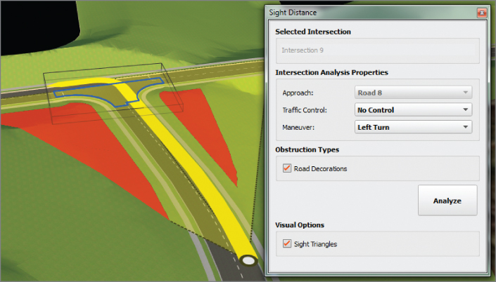
Figure 3.20 An intersection sight distance analysis showing obstructions on both sides

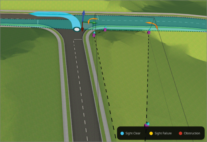
Figure 3.21 A coverage that will be used to grade the area adjacent to an intersection

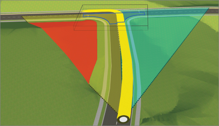
Figure 3.22 An updated analysis after changing the design

Creating Civil 3D Drawings

As you have seen, the Roadway Design for InfraWorks 360 module is an amazingly powerful tool for creating, visualizing, and analyzing your road designs. Even so, the detailed design is still in the hands of AutoCAD Civil 3D software. The View Civil 3D Drawings tool allows you to move your InfraWorks design over to Civil 3D so that you can begin the detailed design phase.

You can find this tool on the Analyze toolbar; when launched, it opens the Create Civil 3D Drawings dialog. This dialog is in the form of a wizard and has three views: Select A Model Road, Select Surface, and Specify Civil 3D Options. The following sections outline the details of the Create Civil 3D Drawings dialog, broken down by view.

The Select A Model Road View

In this view, you configure the Plan Production aspects of the export (see Figure 3.23). What you choose here will determine details (such as sheet size and scale) that will make your final plans look the way you want them to look.

1. Plan Production For A Road Plan Production is a Civil 3D feature that automatically configures and creates the plan and profile sheets for a road. It is a complex feature that automates many Civil 3D and AutoCAD functions. If you're not familiar with this feature, you should definitely read up on it. With this option turned off, the function basically becomes an IMX export that also creates a DWG file.
   1. Road Name Click the Pick A Design Road button and then click your road to select it. You may need to create a proposal with a simplified version of your road so that you can export it using this feature.
   2. Station Range From/To You can restrict your export to a portion of your road, rather than the whole thing. You can supply the station range numerically or by using the pick buttons to choose the start and end locations.
   3. Create Sheets In this section, you will configure precise details for your sheets, such as template, sheet size, layout (plan & profile, plan only, or profile only), and how to distribute the resulting layout tabs (all in one drawing file or distributed across multiple drawing files). These options closely match the Civil 3D choices, so if you are familiar with Civil 3D Plan Production, this will be intuitive.

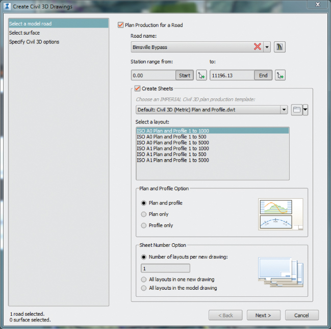
Figure 3.23 The Select A Model Road view of the Create Civil 3D Drawings dialog

The Select Surface View

In this view, you configure the means by which your surface area will be selected (see Figure 3.24).

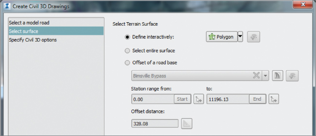
Figure 3.24 The Select Surface view of the Create Civil 3D Drawings dialog

There are three options:

1. Define Interactively This is a selection method you are likely already familiar with because it appears elsewhere in the InfraWorks program. With this option, you can sketch an area by polygon, rectangle, or bounding box.
2. Select Entire Surface Just as it sounds, this option will choose the entire surface represented by your model extent. This choice is not recommended for most models, especially large models. It could cause the export process to take a long time and could generate a large amount of surface data in areas that you don't need.
3. Offset Of A Road Base With this option, you define the surface area by offsetting the centerline of your design road (see Figure 3.25). You can define a station range and offset distance. You can even click the Edit Area Of Interest button to make adjustments to the area after it has been defined by your parameters.

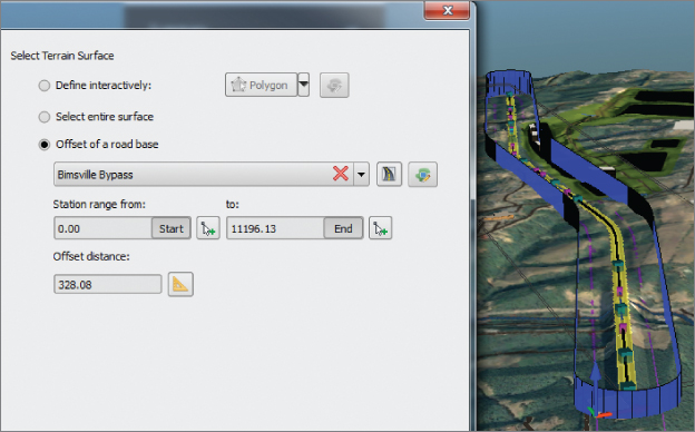
Figure 3.25 Using the Offset Of A Road Base setting

The Specify Civil 3D Options View

In this view, you make some choices relating to the template file and output files that are associated with the export process (see Figure 3.26).

1. Template File Here you choose the template that is used for your main output drawing file. The sheet files that are created will Xref this file.
2. Target File(s) The export process will create DWG files as well as a DST file for the sheet set that will be generated. In this section, you choose the location and filename for each one. Also, you can choose the coordinate system that will be applied to the drawing files.

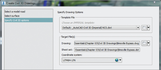
Figure 3.26 The Specify Civil 3D Options view of the Create Civil 3D Drawings dialog

The Final Result

Once you have chosen all of your options in the Create Civil 3D Drawings dialog, you can click Generate and launch the process. The processing time will vary depending on the length of the road and the detail of your terrain surface. Once the process is complete, you will see a dialog that will allow you to view the drawings in the Civil 3D program or open the folder where they have all been stored (see Figure 3.27).

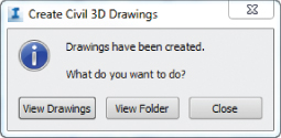
Figure 3.27 The dialog indicating the completion of the process

If you click View Drawings, Civil 3D will open (provided you have Civil 3D installed on your computer), and you will begin at the master drawing. You will also see the Sheet Set Manager palette where you can double-click individual sheets to open them. If you open one of the individual sheets, you should see a fully prepared sheet complete with a layout, title block, viewports, Xref, data references, and many other aspects that have been automatically configured for you (see Figure 3.28).

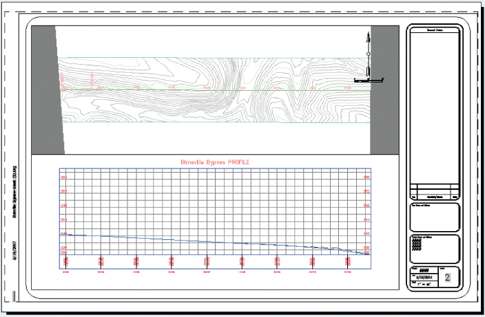
Figure 3.28 A sheet that has been automatically configured by the View Civil 3D Drawings command

From here light-blue you can continue to refine your road designs, provide annotations, and eventually turn out a set of construction documents. The View Civil 3D Drawings command will give you a significant head start on the detailed design process.

Exercise 3.5: Generate Civil 3D Drawings

In this exercise, you will generate plan and profile drawings for a section of the Bimsville Bypass road.

If you are continuing from the previous exercise, you can skip to step 3. Otherwise, if you haven't already done so, go to the book's web page at www.sybex.com/go/roadwaydesignessentials2e and download the files for Chapter 3. Using the instructions in the Introduction, unzip the files to the correct location on your hard drive.

1. If it is not already open, launch the InfraWorks 360 program.
   
2. On InfraWorks 360 Home, click Open. Browse to C:\InfraWorks Roadway Essentials\Chapter 03\. Click Ch03 Bimsville Roads.sqlite and click Open.
3. On the Utility Bar at the top right of your screen, click the Proposals drop-down list and select Ex_3_5.
4. Restore the bookmark named Bimsville Bypass.
5. Click the Roadway Design icon to expand the Roadway Design toolbar.
   
6. On the Roadway Design toolbar, click the Review icon to open the Review toolbar along the left side of the InfraWorks window.
   
7. On the Review toolbar, click Civil 3D Drawings.

   The Create Civil 3D Drawings dialog will open.
   

8. In the Create Civil 3D Drawings dialog, click Select A Model Road and click Pick A Design Road next to Road Name.
   
9. Click the Bimsville Bypass design road in the model.
10. Under Create Sheets, choose Default: Civil 3D (Imperial) Plan And Profile.dwt if you are using imperial units. Choose Default: Civil 3D (Metric) Plan And Profile.dwt if you are using metric units.
11. Review the remaining settings and click Next.
12. In the Select Surface view, verify that Offset Of A Road Base is chosen under Select Terrain Surface.
13. Enter 300 (100) for Offset Distance and then click Next.
14. In the Specify Civil 3D Options view, under Template File, choose Default: _AutoCAD Civil 3D (Imperial) NCS.dwt if you are using imperial units. Choose Default: _AutoCAD Civil 3D (Metric) NCS.dwt if you are using metric units.
15. Under Target File(s), click the folder icon next to Drawing. Browse to C:\InfraWorks Roadway Essentials\Chapter 03\Civil 3D Drawings\ and click Save.
16. Click Generate.

    The command will process for several minutes. When it is complete, a new dialog will appear that gives you the option of viewing the drawings or opening the folder where they are contained.

17. If you have Civil 3D software installed on your computer, click View Drawings. Otherwise, click View Folder and note the files that have been created.
18. If you are able to open the drawings in Civil 3D software, double-click each of the sheets on the Sheet Set Manager palette and study the output.

    You should see sheets that are similar to the ones shown in Figure 3.29.

    You can view the results of successfully completing this exercise by viewing the files located at C:\InfraWorks Roadway Essentials\Chapter 03\Civil 3D Drawings - Complete.

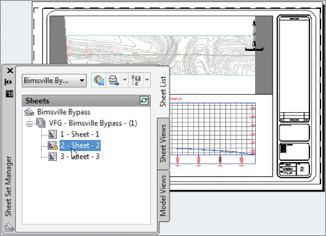
Figure 3.29 The Sheet Set Manager palette along with one of the sheets

---

Now You Know

Now that you have completed this chapter, you can make your InfraWorks roadway designs even better. You know how to optimize your profile to reduce costs while meeting your design requirements. You can also analyze roadways and intersections to identify sight distance issues or to show others that no issues exist. Finally, you are able to efficiently move your InfraWorks road designs to the Civil 3D interface and get a head start on the detailed design process.

Now that you have completed this chapter, you can utilize the advanced roadway design optimization, analysis, and output tools available in the Roadway Design for InfraWorks 360 module.

---