
 BAR CHARTS
DOTPLOTS
HISTOGRAMS
STEMPLOTS
CENTER AND SPREAD
CLUSTERS AND GAPS
OUTLIERS
MODES
SHAPE
CUMULATIVE RELATIVE FREQUENCY PLOTS
SKEWNESS
There are a variety of ways to organize and arrange data. Much information can be put into tables, but these arrays of bare figures tend to be spiritless and sometimes even forbidding. Some form of graphical display is often best for seeing patterns and shapes and for presenting an immediate impression of everything about the data. Among the most common visual representations of data are dotplots, bar charts, histograms, and stemplots. It is important to remember that all graphical displays should be clearly labeled, leaving no doubt what the picture represents—AP Statistics scoring guides harshly penalize the lack of titles and labels!
TIP
The first thing to do with data is to draw a picture—always.
TIP
Just because a variable has numerical values doesn’t necessarily mean that it’s quantitative.
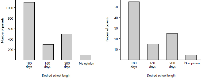
Bar charts are useful with regard to categorical (or qualitative) variables, that is, variables that note the category to which each individual belongs. This is in contrast to quantitative variables, which take on numerical values. Sizes can be measured as frequencies or percents.
 EXAMPLE 1.1
In a survey taken during the first week of January 2015, 1100 parents wanted to keep the school year to the current 180 days, 300 wanted to shorten it to 160 days, 500 wanted to extend it to 200 days, and 100 expressed no opinion. (Or noting that there were 2000 parents surveyed, percentages can be calculated.)
TIP
Graphs must have appropriate labeling and scaling, or they will lose credit!
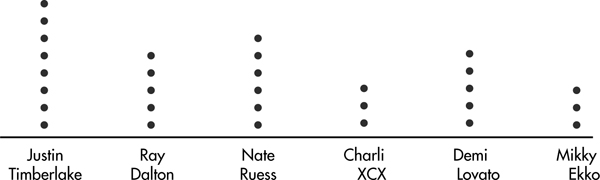
Dotplots can be used with categorical or quantitative variables.
EXAMPLE 1.2
When asked to choose their favorite dance music artist, 8 students chose Justin Timberlake, 5 picked Ray Dalton, 6 picked Nate Ruess, 3 picked Charli XCX, 5 picked Demi Lovato, and 3 picked Mikky Ekko. These data can be displayed in the following dotplot.
EXAMPLE 1.3
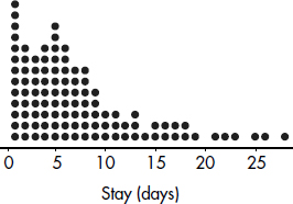
The dotplot below shows the lengths of stay (in days) for all patients admitted to a rural hospital during the first week in January 2015.
Histograms, useful for large data sets involving quantitative variables, show counts or percents falling either at certain values or between certain values. While the AP Statistics Exam does not stress construction of histograms, there are often questions on interpreting given histograms.
To construct a histogram using the TI-84, go to STAT → EDIT and put the data in a list, then turn a STAT PLOT on, choose the histogram icon under Type, specify the list where the data is, and use ZoomStat and/or adjust the WINDOW. Note that XSCL determines the width of the bin or class.
EXAMPLE 1.4
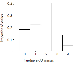
Suppose there are 2200 seniors in a city’s 6 high schools. Four hundred of the seniors are taking no AP classes, 500 are taking one, 900 are taking two, 300 are taking three, and 100 are taking four. These data can be displaced in the following histogram:
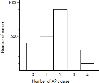
Sometimes, instead of labeling the vertical axis with frequencies, it is more convenient or more meaningful to use relative frequencies, that is, frequencies divided by the total number in the population.
|
Number of AP classes |
Frequency |
Relative frequency |
|
0 |
400 |
400/2200 = 0.18 |
|
1 |
500 |
500/2200 = 0.23 |
|
2 |
900 |
900/2200 = 0.41 |
|
3 |
300 |
300/2200 = 0.14 |
|
4 |
100 |
100/2200 = 0.05 |
Note that the shape of the histogram is the same whether the vertical axis is labeled with frequencies or with relative frequencies. Sometimes we show both frequencies and relative frequencies on the same graph.
EXAMPLE 1.5
Consider the following histogram of the numbers of pairs of shoes owned by 2000 women.
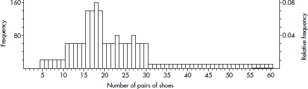
What can we learn from this histogram? For example, none of the women had fewer than 5 or more than 60 pairs of shoes. One hundred sixty of the women had 18 pairs of shoes. Twenty women had 5 pairs of shoes. Half the total area is less than or equal to 19, so half the women have 19 or fewer pairs of shoes. Fifteen percent of the area is more than 30, so 15 percent of the women have more than 30 pairs of shoes. Five percent of the area is more than 50, so 5 percent of the women have more than 50 pairs of shoes.
EXAMPLE 1.6
Consider the following histogram of exam scores, where the vertical axis has not been labeled.
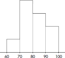
What can we learn from this histogram?
Answer: It is impossible to determine the actual frequencies, that is, we have no idea if there were 25 students, 100 students, or any particular number of students who took the exam. However, we can determine the relative frequencies by noting the fraction of the total area that is over any interval.
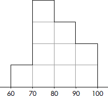
We can divide the area into ten equal portions, and then note that  or 10% of the area is between 60 and 70, so 10% of the students scored between 60 and 70. Similarly, 40% scored between 70 and 80, 30% scored between 80 and 90, and 20% scored between 90 and 100.
Although it is usually not possible to divide histograms so nicely into ten equal areas, the principle of relative frequencies corresponding to relative areas still applies. Also note how this example shows the number of exam scores falling between certain values, whereas the previous two examples showed the number of AP classes taken and number of shoes owned for each value.
TIP
Relative frequencies are the usual choice when comparing distributions of different size populations.
Although a histogram may show how many scores fall into each grouping or interval, the exact values of individual scores are lost. An alternative pictorial display, called a stemplot (also called a stem-and-leaf display) retains this individual information and is useful for giving a quick overview of a distribution, displaying the relative density and shape of the data. A stemplot contains two columns separated by a vertical line. The left column contains the stems, and the right column contains the leaves.
EXAMPLE 1.7
Bisphenol A (BPA) is an industrial chemical that is found in many hard plastic bottles. Recent studies have shown a possible link between BPA exposure and childhood obesity. In one study of 27 elementary school children, urinary BPA levels in nanograms/milliliter (ng/mL) were as follows: {0.2, 0.4, 0.7, 0.7, 0.8, 0.8, 0.9, 1.0, 1.0, 1.3, 1.4, 1.4, 1.4, 1.7, 1.9, 2.1, 2.4, 2.5, 2.8, 2.8, 3.0, 3.3, 3.3, 3.8, 4.2, 4.5, 5.2}
TIP
All stemplots must have keys!
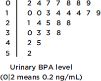
Note: Those with urine BPA level of 2 ng/mL or higher had more than twice the risk of being overweight.
EXAMPLE 1.8
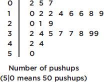
How many nonstop pushups can a 15–18-year-old teenager do? In one study in a mixed gender high school gym class, the numbers of pushups were {2, 5, 7, 10, 12, 12, 14, 16, 16, 18, 19, 20, 21, 29, 32, 34, 35, 37, 37, 38, 39, 39, 42, 44, 50}
TIP
Center and spread should always be described together.
Looking at a graphical display, we see that two important aspects of the overall pattern are
1. the center, which separates the values (or area under the curve in the case of a histogram) roughly in half, and
2. the spread, that is, the scope of the values from smallest to largest.
In the histogram of Example 1.4, the center is 2 AP classes while the spread is from 0 to 4 AP classes.
In the histogram of Example 1.5 the center is about 19, and the spread is from 5 to 60; in the histogram of Example 1.6, the center is about 80, and the spread is from 60 to 100.
In the stemplot of Example 1.7, the center is 1.7 (middle of the 27 values), and the spread is from 0.2 to 5.2; in the stemplot of Example 1.8, the center is 21 (middle of the 25 values), and the spread is from 2 to 50.
Other important aspects of the overall pattern are
1. clusters, which show natural subgroups into which the values fall (for example, the salaries of teachers in Ithaca, NY, fall into three overlapping clusters, one for public school teachers, a higher one for Ithaca College professors, and an even higher one for Cornell University professors), and
2. gaps, which show holes where no values fall (for example, the Office of the Dean sends letters to students being put on the honor roll and to those being put on academic warning for low grades; thus the GPA distribution of students receiving letters from the Dean has a huge middle gap).
EXAMPLE 1.9
Hodgkin’s lymphoma is a cancer of the lymphatic system, the system that drains excess fluid from the blood and protects against infection. Consider the following histogram:
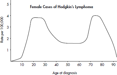
Simply saying that the average age at diagnosis for female cases is around 50 clearly misses something. The distribution of ages at diagnosis for female cases of Hodgkin’s lymphoma is bimodal with two distinct clusters, centered at 25 and 75.
TIP
Pay attention to outliers!
Extreme values, called outliers, are found in many distributions. Sometimes they are the result of errors in measurements and deserve scrutiny; however, outliers can also be the result of natural chance variation. Outliers may occur on one side or both sides of a distribution.
Some distributions have one or more major peaks, called modes. (The values with the peaks above them are the modes.) With exactly one or two such peaks, the distribution is said to be unimodal or bimodal, respectively. But every little bump in the data is not a mode! You should always look at the big picture and decide whether or not two (or more) phenomena are affecting the histogram.
TIP
Some distributions have many little ups (and downs), which should not be confused with modes.
EXAMPLE 1.10
The histogram below shows employee computer usage (number accessing the Internet) at given times at a company main office.
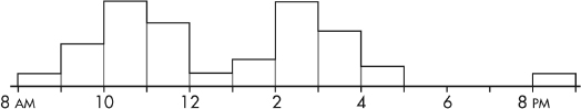
Note that this is a bimodal distribution. Computer usage at this company appears heaviest at midmorning and midafternoon, with a dip in usage during the noon lunch hour. There is an evening outlier possibly indicating employees returning after dinner (or perhaps custodial cleanup crews taking an Internet break!).
Note that, as illustrated above, it is usually instructive to look for reasons behind outliers and modes.
TIP
When describing a distribution, always comment on Shape, Outliers, Center, and Spread (SOCS). Or, alternatively, Center, Unusual values, Shape, and Spread (CUSS). And always describe in context.
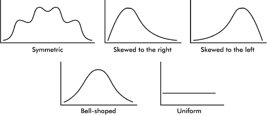
Distributions come in an endless variety of shapes; however, certain common patterns are worth special mention:
1. A symmetric distribution is one in which the two halves are mirror images of each other. For example, the weights of all people in some organizations fall into symmetric distributions with two mirror-image bumps, one for men’s weights and one for women’s weights.
2. A distribution is skewed to the right if it spreads far and thinly toward the higher values. For example, ages of nonagenarians (people in their 90s) is a distribution with sharply decreasing numbers as one moves from 90-year-olds to 99-year-olds.
3. A distribution is skewed to the left if it spreads far and thinly toward the lower values. For example, scores on an easy exam show a distribution bunched at the higher end with few low values.
4. A bell-shaped distribution is symmetric with a center mound and two sloping tails. For example, the distribution of IQ scores across the general population is roughly symmetric with a center mound at 100 and two sloping tails.
5. A distribution is uniform if its histogram is a horizontal line. For example, tossing a fair die and noting how many spots (pips) appear on top yields a uniform distribution with 1 through 6 all equally likely.
Even when a basic shape is noted, it is important also to note if some of the data deviate from this shape.
TIP
In the real world, distributions are rarely perfectly symmetric or perfectly uniform, so we usually say “roughly” or “approximately” symmetric or uniform.
CUMULATIVE RELATIVE FREQUENCY PLOTS
Sometimes we sum frequencies and show the result visually in a cumulative relative frequency plot (also known as an ogive).
EXAMPLE 1.11
The following graph shows 2015 school enrollment in the United States by age.
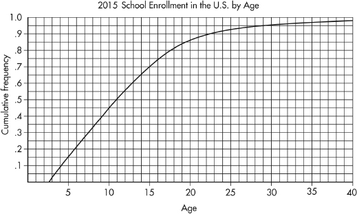
What can we learn from this cumulative relative frequency plot? For example, going up to the graph from age 5, we see that 0.15 or 15% of school enrollment is below age 5. Going over to the graph from 0.5 on the vertical axis, we see that 50% of the school enrollment is below and 50% is above a middle age of 11. Going up from age 30, we see that 0.95 or 95% of the enrollment is below age 30, and thus 5% is above age 30. Going over from 0.25 and 0.75 on the vertical axis, we see that the middle 50% of school enrollment is between ages 6 and 7 at the lower end and age 16 at the upper end.
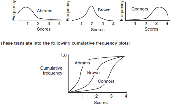
CUMULATIVE RELATIVE FREQUENCY AND SKEWNESS
A distribution skewed to the left has a cumulative frequency plot that rises slowly at first and then steeply later, while a distribution skewed to the right has a cumulative frequency plot that rises steeply at first and then slowly later.
EXAMPLE 1.12
Consider the essay grading policies of three teachers, Abrams, who gives very high scores, Brown, who gives equal numbers of low and high scores, and Connors, who gives very low scores. Histograms of the grades (with 1 the highest score and 4 the lowest score) are as follows:
SUMMARY
 The three keys to describing a distribution are shape, center, and spread.
Also consider clusters, gaps, modes, and outliers.
Always provide context.
Look for reasons behind any unusual features.
A few common shapes arise from symmetric, skewed to the right, skewed to the left, bell-shaped, and uniform distributions.
For categorical (qualitative) data, dotplots and bar charts give useful displays.
For quantitative data, histograms, cumulative relative frequency plots (ogives), and stemplots give useful displays.
In a histogram, relative area corresponds to relative frequency.
QUESTIONS ON TOPIC ONE: GRAPHICAL DISPLAYS
Multiple-Choice Questions
Directions: The questions or incomplete statements that follow are each followed by five suggested answers or completions. Choose the response that best answers the question or completes the statement.
1. The stemplot below shows ages of CEOs of a select group of corporations.
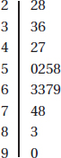
Which of the following is not a correct statement about this distribution?
(A) The distribution is bell-shaped.
(B) The distribution is skewed left and right.
(C) The center is around 60.
(D) The spread is from 22 to 90.
(E) There are no outliers.
2. Which of the following is a true statement?
(A) Stemplots are useful both for quantitative and categorical data sets.
(B) Stemplots are equally useful for small and very large data sets.
(C) Stemplots can show symmetry, gaps, clusters, and outliers.
(D) Stemplots may or may not show individual values.
(E) Stems may be skipped if there is no data value for a particular stem.
3. Which of the following is an incorrect statement?
(A) In histograms, relative areas correspond to relative frequencies.
(B) In histograms, frequencies can be determined from relative heights.
(C) Symmetric histograms may have multiple peaks.
(D) Two students working with the same set of data may come up with histograms that look different.
(E) Displaying outliers may be more problematic when using histograms than when using stemplots.
4. Following is a histogram of test scores.
Which of the following is a true statement?
(A) The middle (median) score was 75.
(B) The mean score was 70.
(C) The mean score is probably less than the median score.
(D) If the passing score was 60, most students failed.
(E) More students scored between 50 and 60 than between 90 and 100.
Questions 5–9 refer to the following five cumulative relative frequency plots:
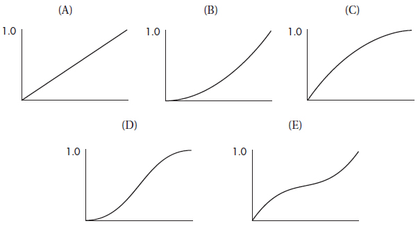
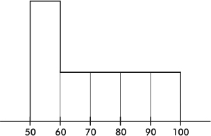
5. To which of the above cumulative relative frequency plots does the following histogram correspond?
(A) A
(B) B
(C) C
(D) D
(E) E
6. To which of the above cumulative relative frequency plots does the following histogram correspond?
(A) A
(B) B
(C) C
(D) D
(E) E
7. To which of the above cumulative relative frequency plots does the following histogram correspond?
(A) A
(B) B
(C) C
(D) D
(E) E
8. To which of the above cumulative relative frequency plots does the following histogram correspond?
(A) A
(B) B
(C) C
(D) D
(E) E
9. To which of the above cumulative relative frequency plots does the following histogram correspond?
(A) A
(B) B
(C) C
(D) D
(E) E
Free-Response Questions
Directions: You must show all work and indicate the methods you use. You will be graded on the correctness of your methods and on the accuracy of your final answers.
THREE OPEN-ENDED QUESTIONS
1. The dotplot below shows the numbers of goals scored by the 20 teams playing in a city’s high school soccer games on a particular day.
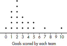
(a) Describe the distribution.
(b) One superstar scored six goals, but his team still lost. What are all possible final scores for that game? Explain.
(c) Is it possible that all the teams scoring exactly two goals won their games? Explain.
2. The winning percentages for a major league baseball team over the past 22 years are shown in the following stemplot:
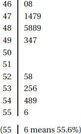
(a) Interpret the lowest value.
(b) Describe the distribution.
(c) Give a reason that one might argue that the team is more likely to lose a given game than win it.
(d) Give a reason that one might argue that the team is more likely to win a given game than lose it.
3. A college basketball team keeps records of career average points per game of players playing at least 75% of team games during their college careers. The cumulative relative frequency plot below summarizes statistics of players graduating over the past 10 years.
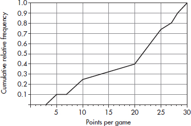
(a) Interpret the point (20, 0.4) in context.
(b) Interpret the intersection of the plot with the horizontal axis in context.
(c) Interpret the horizontal section of plot from 5 to 7 points per game in context.
(d) The players with the top 10% of the career average points per game achievements will be listed on a plaque. What is the cutoff score for being included on the plaque?
(e) What proportion of the players averaged between 10 and 20 points per game?
AN INVESTIGATIVE TASK
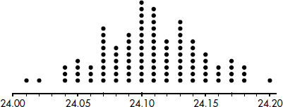
A company engineer creates a diagnostic measurement, 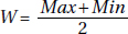 , which should be at least 24.10 in a sample of size 12 if certain machinery is operating correctly. To explore this diagnostic measurement, the machine is perfectly calibrated. Then 100 random samples of size 12 of the product are taken from the assembly line. For each of these 100 samples, the diagnostic measurement W is calculated and shown plotted below.
Each day, one sample of size 12 is taken from the assembly line and the diagnostic measurement W is calculated. If W drops too low, a decision to recalibrate the machinery is made.
(a) From the dotplot above, estimate a measure of center and a measure of variability for the distribution.
(b) For the dotplot above, do there appear to be any outliers (no calculations required)? Justify your answer.
One day the random sample is {24.2, 24.84, 25.05, 23.43, 23.9, 25.01, 23.01, 24.5, 24.23, 23.76, 24.69, 23.21}.
(c) Based on the dotplot above, does the engineer have sufficient evidence to conclude that recalibration is necessary? Justify your answer.