 which in this case gives
Diagnostic Examination
SECTION I
1. (A) Without knowing the actual number of points scored each season, only proportions, not numbers of points, can be compared between seasons.
2. (C) The critical t-values with df = 20 – 2 = 18 are ± 2.878. Thus, we have b1 ± t∗ × SE(b1) = 4.0133 ± (2.878)(0.4922).
3. (A) The shortest sequence has a greater probability than any longer sequence.
4. (A) Power, the probability of rejecting a false null hypothesis, will be the greatest for parameter values farthest from the hypothesized value, in the direction of the alternative hypothesis.
5. (A) A simple random sample may or may not be representative of the population. It is a method of selection in which every possible sample of the desired size has an equal chance of being selected.
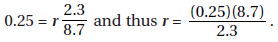
6. (A) A formula relating the given statistics is which in this case gives
7. (B) The null hypothesis is that the new medication is no better than insulin injection, while the alternative hypothesis is that the new medication is better. A Type I error means a mistaken rejection of a true null hypothesis.
8. (D) A Type II error means a mistaken failure to reject a false null hypothesis.
9. (C) Running a hypothesis test at the 5% significance level means that the probability of committing a Type I error is 0.05. Then the probability of not committing a Type I error is 0.95. Assuming the tests are independent, the probability of not committing a Type I error on any of the five tests is (0.95)5 = 0.77378, and the probability of at least one Type I error is 1 – 0.77378 = 0.22622.
10. (E) No matter what the distribution of raw scores, the set of z-scores always has mean 0 and standard deviation 1.
11. (B) In the sampling distribution of x, the mean is equal to the population mean, and the standard deviation is equal to the population standard deviation divided by the
square root of the sample size, in this case, 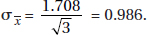
12. (E) The standard deviation can never be negative.
13. (E) When a complete census is taken (all 423 seniors were in the study), the population proportion is known and a confidence interval has no meaning.
14. (E) The method described in (A) is a convenience sample, (B) and (C) are voluntary response surveys, and (D) suffers from undercoverage bias.
15. (D) Since each set is normally distributed so is the set of differences, X1 – X2. We calculate µx1 – x2 = 1758 – 1725 = 33 and 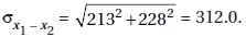
So 
16. (E) With df = n – 1 = 10 – 1 = 9 and 95% confidence, the critical t-values are ±2.262.
Also 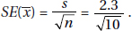
17. (A) 
 , …, and we see that the distribution has its maximum value
at X = 1.
18. (B) The chi-square tests all involve counts, and comparing means doesn’t make sense in this context.
19. (A) The median of X is –2, and this is also true of distribution 1 (note that a horizontal line from 0.5 strikes curve 1 above –2 on the x-axis). Y has a smaller standard deviation than Z (tighter clustering around the mean), so Y must correspond to distribution 2, which shows almost all values are between –1 and 1.
20. (E)
21. (C) Adding the same constant to every value in a set adds the same constant to the mean but leaves the standard deviation unchanged. Multiplying every value in a set by the same constant multiplies the mean and standard deviation by that constant. So the new mean is 5/9 × (78.35 – 32) + 273 = 298.75, and the new standard deviation is 5/9 × 6.3 = 3.5.
22. (B) Design 2 is an example of a matched pairs design, a special case of a block design; here, each subject is compared to itself with respect to the two treatments. Both designs definitely use randomization with regard to assignment of treatments, but since they do not use randomization in selecting subjects from the general population, care must be taken in generalizing any conclusions. It’s not clear whether or not the researchers who do the observations and measurements know which treatment individual cows are receiving, so there is no way to conclude if there is or is not blinding. The two sources of BVH are different treatments, and so they are not being confounded. In both designs treatments are randomly applied, so neither is an observational study.
23. (A) The linear regression t-test has null hypothesis H0:  = 0 that there is no linear relationship; if the P-value is small enough, then there is evidence of a linear association, that is, there is evidence that ≠ 0.
24. (A) We have a binomial distribution with mean  Answer
(A) is the only reasonable choice.
25. (B) The size of the sample always matters; the larger the sample, the greater the power of statistical tests. One percent of a large population is large. Larger samples are better, but if the sample is greater than 10% of the population, the best statistical techniques are not those covered in the AP curriculum.
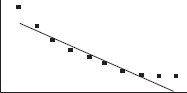
26. (E) The points on the scatterplot all fall on the straight line:
Female length = Male length + 0.5
27. (A) 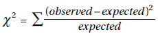 and expected are found by multiplying the proportions times the sample size of 100.
28. (D) The distributions in (A), (B), and (C) appear roughly symmetric, so the mean and median will be roughly the same. The distribution in (D) is skewed to the right, so the mean will be greater than the median, while the distribution in (E) is skewed to the left, so the mean will be less than the median.
29. (C) This is a binomial with n = 10 and p = 0.38, so the mean is np = 10(0.38) = 3.8.
30. (E) Answers (A), (B), and (C) are common misconceptions. Since the 95% confidence interval contains 80, a two-sided test would not be significant at the 5% significance level or lower. The interval can be expressed as 77.5 ± 3, that is, we are 95% confident that the true mean fastball speed is within 3 mph of 77.5 mph.
31. (A) Residual = Observed – Predicted, so 1.0 = 11 – Predicted and Predicted = 10.
32. (B) Stratified sampling is when the population is divided into homogeneous groups (the three Divisions in this example), and a random sample of individuals is chosen from each group.
33. (D) There are 8 outcomes {TTT, TTH, THT, THH, HTT, HTH, HHT, HHH}, so P(0 heads) = 1/8, P(1 head) = 3/8, P(2 heads) = 3/8, and P(3 heads) = 1/8. Thus, we assign one digit to the results of 0 heads and 3 heads and 3 digits to the results of 1 head and 2 heads and ignore the other 2 digits (of the 10 available digits).
34. (A) The margin of error,  depends on the sample size, not the population size.
35. (B) We have (Q1 + Q3)/2 = 20 or Q3 + Q1 = 40, and Q3 – Q1 = 20, which algebraically gives Q1 = 10 and Q3 = 30 [add the equations to obtain 2Q3 = 60 so Q3 = 30; then plugging into either equation and solving for Q1 gives Q1 = 10].
36. (E) The larger the sample size, the closer the sample distribution is to the population distribution. The central limit theorem roughly says that if multiple samples of size n are drawn randomly and independently from a population, then the histogram of the means of those samples will be approximately normal. Statistics have probability distributions called sampling distributions. The standard error is based on the spread of the population and on the sample size. The central limit theorem does not apply to all statistics as it does to sample means. Many sampling distributions are not normal; for example, the sampling distribution of the sample max is not a normal distribution. An estimator of a parameter is unbiased if we have a method that, through repeated samples, is on average the same value as the parameter.
37. (A) With 0.068 in a tail, the confidence interval with 34 at one end would have a confidence level of 1 – 2(0.068) = 0.864, so anything higher than 86.4% confidence will contain 34.
38. (C) From a boxplot there is no way of telling if a distribution is bell-shaped (very different distributions can have the same five-number summary). Distribution I appears strongly skewed right, and so its mean is probably much greater than its median, while distribution II appears roughly symmetric, and so its mean is probably close to its median. The interquartile range, not the range, in I is 13.
39. (C) To make money, there must be more wins than losses, so with 50 plays, we need to calculate P(X > 25). We have a binomial distribution with n = 50 and probability of success p = 18/38. On a calculator such as the TI-84 we find P(X > 25) = 1 – P(X ≤ 25) = 1-binomcdf(50,18/38,25) = 0.303 [or on the Nspire: binomcdf(50,18/38,26,50)].
40. (B)  and cell calculations [expected value of a cell equals (row total)(column total)/(table total)] or
  2-test on a calculator such as the TI-84 will yield expected cells of 29, 36, 35, 29, 36, 35.
SECTION II
1. (a) There are 2 × 2 × 2 = 8 different treatments:
Two-day, aerobic, with adjuvant
Two-day, aerobic, without adjuvant
Two-day, anaerobic, with adjuvant
Two-day, anaerobic, without adjuvant
Five-day, aerobic, with adjuvant
Five-day, aerobic, without adjuvant
Five-day, anaerobic, with adjuvant
Five-day, anaerobic, without adjuvant
(b) We must randomly assign the treatment combinations to the beds. (Roses have already been randomly assigned to the beds.) With 8 treatments and 16 beds, each treatment should be assigned to 2 beds. For example, give each bed a random number between 1 and 16 (no repeats), and then assign the first treatment in the above list to the beds with the numbers 1 and 2, assign the second treatment in the above list to the beds with the numbers 3 and 4, and so on.
(c) Using only mini-pink roses in this experiment gives reduced variability and increases the likelihood of determining differences among the treatments.
(d) Using only mini-pink roses in this experiment limits the scope and makes it difficult to generalize the results to other species of roses.
SCORING
Part (a) is essentially correct for correctly listing all eight treatment combinations and is incorrect otherwise.
Part (b) is essentially correct if each treatment combination is randomly assigned to two beds of roses. Part (b) is partially correct if each treatment is randomly assigned to two beds but the method is unclear, or if a method of randomization is correctly described but the method may not assure that each treatment is assigned to two beds.
Part (c) is essentially correct for noting reduced variability and for explaining that this increases likelihood of determining differences among the treatments. Part (c) is partially correct for only one of these two components.
Part (d) is essentially correct noting limited scope and for explaining that this makes generalization to other species difficult. Part (d) is partially correct for only one of these two components.
Count partially correct answers as one-half an essentially correct answer.
4 Complete Answer |
Four essentially correct answers. |
3 Substantial Answer |
Three essentially correct answers. |
2 Developing Answer |
Two essentially correct answers. |
1 Minimal Answer |
One essentially correct answer. |
Use a holistic approach to decide a score totaling between two numbers.
TIP
Graders want to give you credit. Help them! Make them understand what you are doing, why you are doing it, and how you are doing it. Don’t make the reader guess at what you are doing. Communication is just as important as statistical knowledge!
2. Part 1: State the correct hypotheses.
H0 : µ = 82 and Ha : µ > 82
Part 2: Identify the correct test and check appropriate conditions.
One-sample 
Conditions: Random sample (given), n = 47 is less than 10% of all possible swings with the new racquet, and n = 47 is sufficiently large for the CLT to apply.
Part 3: Calculate the test statistic t and the P-value.
Calculator software (such as T-Test on the TI-84) gives t = 3.0246 and P = 0.00203.
Part 4: Give a conclusion in context with linkage to the P-value.
With this small a P-value, 0.00203 < 0.05, there is sufficient evidence to reject H0, that is, there is sufficient evidence that his mean speed with the new racquet is an improvement over the old.
SCORING
Part 1 either is essentially correct or is incorrect.
Part 2 is essentially correct if the test is correctly identified by name or formula and the assumptions are checked. Part 2 is partially correct if only one of these two elements is correct.
Part 3 is essentially correct if the t-value and p are stated. Part 3 is partially correct if only one of these two elements is correct.
Part 4 is essentially correct if the correct conclusion is given in context and the conclusion is linked to the p-value. Part 4 is partially correct if the correct conclusion is given in context but there is no linkage to the p-value.
Count partially correct answers as one-half an essentially correct answer.
4 Complete Answer |
Four essentially correct answers. |
3 Substantial Answer |
Three essentially correct answers. |
2 Developing Answer |
Two essentially correct answers. |
1 Minimal Answer |
One essentially correct answer. |
Use a holistic approach to decide a score totaling between two numbers.
3. (a) Chi-square goodness-of-fit test
(b) H0: The new freshman class is distributed 2.7% non-Hispanic Black, 3.7% Asian or Pacific Islander, 4.0% Hispanic, 80.0% non-Hispanic White, and 9.6% other/unknown.
Ha: The new freshman class has a distribution different from that in October 2008.
Randomization is given and the expected cell frequencies—2.7% × 200 = 5.4, 3.7% × 200 = 7.4, 4.0% × 200 = 8.0, 80.0% × 200 = 160.0, and 9.6% × 200 = 19.2—are all at least 5.
(c)
with df = 5 – 1 = 4, and a P-value of 0.013. With such a small P-value, 0.013 < 0.05, there is evidence to reject H0 and conclude that there is statistical evidence of a change in ethnic/racial composition.
(d) No, this test/procedure targeted students visiting the campus, and such students might be different from the targeted population of students making up the new freshman class. For example, some students who eventually make up the freshman class might not have the funds or the time to visit the campus. Or it can be argued that even if all potential students do visit the campus, there is no reason to conclude that the distribution of visiting students is the same as the distribution of students who both are accepted and decide to attend this college.
SCORING
Part (a–b) is essentially correct if the correct test is named, the hypotheses are correctly stated, and the assumption of all expected cell frequencies being at least five is checked. Part (a–b) is partially correct if only two of these three elements are correct. Part (a–b) is incorrect if only one of these three elements is correct.
Part (c1) is essentially correct if the chi-square value is calculated and both df and p are stated. Part (c1) is partially correct if only one of these two elements is correct.
Part (c2) is essentially correct if the correct conclusion is given in context and the conclusion is linked to the p-value. Part (c2) is partially correct if the correct conclusion is given in context but there is no linkage to the p-value.
Part (d) is essentially correct or incorrect. It is essentially correct for both stating that the intended population is not targeted and giving a clear argument for this answer.
Count partially correct answers as one-half an essentially correct answer.
4 Complete Answer |
Four essentially correct answers. |
3 Substantial Answer |
Three essentially correct answers. |
2 Developing Answer |
Two essentially correct answers. |
1 Minimal Answer |
One essentially correct answer. |
Use a holistic approach to decide a score totaling between two numbers.
4. (a) 
(b) P(at least 3 out of 5 are > 2400) = 10(0.258)3(0.742)2 + 5(0.258)4(0.742) + (0.258)5 = 0.112
[On the TI-84, 1 – binomcdf(5,0.258,2) = 0.112]
(c) The distribution of x is normal with mean µx = 2317 and standard deviation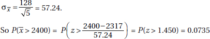
SCORING
Part (a) is essentially correct if the correct probability is calculated and the derivation is clear. Simply writing normalcdf(2400, ,2317,128) = 0.258 is a partially correct response.
Part (b) is essentially correct if the correct probability is calculated and the derivation is clear. Part (b) is partially correct for indicating a binomial with n = 5 and p = answer from (a) but calculating incorrectly. Simply writing 1-binomcdf(5,.258,2) = 0.112 is also a partially correct response.
Part (c) is essentially correct for specifying both  and
and  and correctly calculating the probability. Part (c) is partially correct for specifying both and but incorrectly calculating the probability, or for failing to specify both and but correctly calculating the probability.
4 Complete Answer |
All three parts essentially correct. |
3 Substantial Answer |
Two parts essentially correct and one part partially correct. |
2 Developing Answer |
Two parts essentially correct OR one part essentially correct and one or two parts partially correct OR all three parts partially correct. |
1 Minimal Answer |
One part essentially correct OR two parts partially correct. |
5. (a)  xP(x) = 135p + (–35)(1 – p) = –35 + 170p
(b) xP(x) = (–5)p + 25(1 – p) = 25 – 30p
(c) –35 + 170p = 25 – 30p gives p = 0.3. When p > 0.3, the expected return for oil paintings is greater than that for finger paintings, and when p < 0.3, the expected return for finger paintings is greater than for oil paintings. (These statements follow from the positive slope of R = –35 + 170p and the negative slope of R = 25 – 30p.)
(d) First, name the confidence interval: a 95% confidence interval for the proportion p of similar establishments with tourists who were primarily art collectors.
Second, check conditions: We are given that this is a random sample, it is reasonable to assume that the sample is less than 10 percent of all similar establishments, and the sample size is large enough (np = 33 and n(1 – p) = 117 are both greater than 10).
Third, correct mechanics: calculator software (such as 1-PropZInt on the TI-84) gives (0.154, 0.286).
Fourth, interpret in context: We are 95% confident that the true proportion of similar establishments with tourists who were primarily art collectors is between 0.154 and 0.286.
(e) The entire interval in (d) is below p = 0.3, so based on (c), the expected return for finger paintings is greater than for oil paintings for all p in this interval.
SCORING
Parts (a) and (b) are scored together. They are essentially correct if both answers are correct and partially correct if one answer is correct.
Part (c) is essentially correct for a correct calculation of the intersection together with a correct conclusion of what it means when p is greater or less than 0.3. Part (c) is partially correct if the intersection is not correctly calculated, but the conclusions are correct based on the incorrect intersection value.
Part (d) is essentially correct if steps 2, 3, and 4 are correct. (Step 1 is only a restatement from the question.) Part 3 is partially correct if only two of these three steps are correct.
Part (e) is essentially correct if the correct conclusion is given with clear linkage to the results from both (c) and (d). Part (e) is partially correct if the explanation of the linkage is present but weak.
Give 1 point for each essentially correct part and one-half point for each partially correct part.
4 Complete Answer |
4 points |
3 Substantial Answer |
3 points |
2 Developing Answer |
2 points |
1 Minimal Answer |
1 point |
Use a holistic approach to decide a score totaling between two numbers.
TIP
Read carefully and recognize that sometimes very different tests are required in different parts of the same problem.
Section II
Part B
6. (a) Salary and years of experience exhibit an approximately linear relationship. As years of experience increase, so does the median salary. The third-quartile, Q3, salary also increases with years, and so does the Q1 salary with the exception of one year. As years of experience increase, there are only minor differences in measures of variability in the salaries, with roughly the same range (except for the last two) and fairly consistent interquartile ranges.
(b) First, the boxplots indicate that an overall scatterplot pattern would be roughly linear. Second, the residual plot shows no pattern. Third, the histogram of residuals appears roughly normal (unimodal, symmetric, and without clear skewness or outliers).
(c) With df = 98 and 0.025 in each tail, the critical t-values are ±1.984.
b1 ± tsb1 = 0.910 ± 1.984(0.03273) = 0.910 ± 0.065. We are 95% confident that for each additional year of experience, the average increase in salary is between $845 and $975.
(d) The sum and thus the mean of the residuals is always 0. The standard deviation of the residuals is  , which can be estimated with s = 0.9402. With a roughly normal distribution, we have P(X
  1) = 0.14.
SCORING
Part (a) is essentially correct for correctly noting a linear relationship, noting that as years of experience increase so does the median salary (or Q3 or generally Q1), and noting that measures of variability (range or IQR) stay roughly the same. Part (a) is partially correct for correctly noting two of the three features.
Part (b) is essentially correct for noting the three conditions (roughly linear scatterplot, no pattern in the residual plot, and roughly normal histogram of residuals). Part (b) is partially correct for correctly noting two of the three conditions.
Part (c) is essentially correct for both a correct calculation of the confidence interval and a correct interpretation in context. Part (c) is partially correct for a correct calculation without the interpretation in context, or for a correct interpretation based on an incorrect calculation.
Part (d) is essentially correct noting that the distribution of residuals is roughly normal with mean 0 and standard deviation 0.9402, and then using this to correctly calculate the probability. Part (d) is partially correct for correctly noting the distribution of residuals but incorrectly calculating the probability, or for making a calculation based on a normal distribution with mean 0 but using an incorrect standard deviation.
Count partially correct answers as one-half an essentially correct answer.
4 Complete Answer |
Four essentially correct answers. |
3 Substantial Answer |
Three essentially correct answers. |
2 Developing Answer |
Two essentially correct answers. |
1 Minimal Answer |
One essentially correct answer. |
Use a holistic approach to decide a score totaling between two numbers.
1 Graphical Displays
Answers Explained
MULTIPLE-CHOICE
1. (B) There is no such thing as being skewed both left and right.
2. (C) Stemplots are not used for categorical data sets, are too unwieldy to be used for very large data sets, and show every individual value. Stems should never be skipped over—gaps are important to see.
3. (B) Histograms give information about relative frequencies (relative areas correspond to relative frequencies) and may or may not have an axis with actual frequencies. Symmetric histograms can have any number of peaks. Choice of width and number of classes changes the appearance of a histogram. Stemplots clearly show outliers; however, in histograms outliers may be hidden in large class widths.
4. (E) The median score splits the area in half, and so the median is not 75. The median appears to be about 70 (with equal area on each side), and since the data are skewed right, the mean will be larger than the median, so the mean is greater than 70. The area between 50 and 60 is greater than the area between 90 and 100 but is less than the area between 60 and 100.
5. (B) A histogram with little area under the curve early and much greater area later results in a cumulative relative frequency plot which rises slowly at first and then at a much faster rate later.
6. (C) A histogram with large area under the curve early and much less area later results in a cumulative relative frequency plot which rises quickly at first and then at a much slower rate later.
7. (E) A histogram with little area under the curve in the middle and much greater area on both ends results in a cumulative relative frequency plot which rises quickly at first, then almost levels off, and finally rises quickly at the end.
8. (D) A histogram with little area under the curve on the ends and much greater area in the middle results in a cumulative relative frequency plot which rises slowly at first, then quickly in the middle, and finally slowly again at the end.
9. (A) Uniform distributions result in cumulative relative frequency plots which rise at constant rates, thus linear.
FREE-RESPONSE
1. (a) A complete answer considers shape, center, and spread.
Shape: unimodal, skewed right, outlier at 10
Center: around 2 or 3
Spread: from 0 to 10
(b) If the player scored six goals, his/her team must have scored either 7 or 10, but they lost, so they scored 7, and the only possible final score is that they lost by a score of 10 to 7.
(c) No, there were six teams that scored exactly two goals, but there were only five teams that scored less than two goals, so not all the two-goal teams could have won.
2. (a) The lowest winning percentage over the past 22 years is 46.0%.
(b) A complete answer considers shape, center, and spread.
Shape: two clusters, each somewhat bell-shaped
Center: around 50%
Spread: from 46.0 to 55.6%
(c) The team had more losing seasons (13) than winning seasons (9).
(d) The cluster of winning percentages is further above 50% than the cluster of losing percentages is below 50%.
3. (a) 40% of the players averaged fewer than 20 points per game.
(b) All the players averaged at least 3 points per game.
(c) No players averaged between 5 and 7 points per game because the cumulative relative frequency was 10% for both 5 and 7 points.
(d) Go over to the plot from 0.9 on the vertical axis, and then down to the horizontal axis to result in 28 points per game.
(e) Reading up to the plot and then over from 10 and from 20 shows that 0.25 of the players averaged under 10 points per game and 0.4 of the players averaged under 20 points per game. Thus, 0.4 – 0.25 = 0.15 gives the proportion of players who averaged between 10 and 20 points per game.
AN INVESTIGATIVE TASK
(a) The center is roughly between 24.10 and 24.11, and the data are spread from 24.01 to 24.20.
(b) There seems to be two “low” data points, 24.01 and 24.02, and one “high” data point, 24.20. These three data points are distinctly separated from the other points.
(c) For this day’s sample, 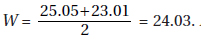 A value of 24.03 or less occurred only twice in the 100 samples. Thus, if the machinery was operating properly, a W measurement of 24.03 would be very unusual. The conclusion should be to recalibrate the machine.
2 Summarizing Distributions
Answers Explained
MULTIPLE-CHOICE
1. (D) The distribution is clearly skewed right, so the mean is greater than the median, and the ratio is greater than one.
2. (E) All elements of the sample are taken from the population, and so the smallest value in the sample cannot be less than the smallest value in the population; similarly, the largest value in the sample cannot be greater than the largest value in the population. The interquartile range is the full distance between the first quartile and the third quartile. Outliers are extreme values, and while they may affect the range, they do not affect the interquartile range when the lower and upper quarters have been removed before calculation.
3. (E) Outliers are any values below Q1 – 1.5(IQR) = 5.5 or above Q3 + 1.5(IQR) = 57.5.
4. (A) The value 50 seems to split the area under the histogram in two, so the median is about 50. Furthermore, the histogram is skewed to the left with a tail from 0 to 30.
5. (B) Looking at areas under the curve, Q1 appears to be around 20, the median is around 30, and Q3 is about 40.
6. (C) Looking at areas under the curve, Q1 appears to be around 10, the median is around 30, and Q3 is about 50.
7. (C) The boxplot indicates that 25% of the data lie in each of the intervals 10–20, 20–35, 35–40, and 40–50. Counting boxes, only histogram C has this distribution.
8. (D) The boxplot indicates that 25% of the data lie in each of the intervals 10–15, 15–25, 25–35, and 35–50. Counting boxes, only histogram D has this distribution.
9. (E) The boxplot indicates that 25% of the data lie in each of the intervals 10–20, 20–30, 30–40, and 40–50. Counting boxes, only histogram E has this distribution.
10. (A) Subtracting 10 from one value and adding 5 to two values leaves the sum of the values unchanged, so the mean will be unchanged. Exactly what values the outliers take will not change what value is in the middle, so the median will be unchanged.
11. (C) The high outlier is further from the mean than is the low outlier, so removing both will decrease the mean. However, removing the lowest and highest values will not change what value is in the middle, so the median will be unchanged.
12. (C) Adding the same constant to every value increases the mean by that same constant; however, the distances between the increased values and the increased mean stay the same, and so the standard deviation is unchanged. Graphically, you should picture the whole distribution as moving over by a constant; the mean moves, but the standard deviation (which measures spread) doesn’t change.
13. (E) Multiplying every value by the same constant multiplies both the mean and the standard deviation by that constant. Graphically, increasing each value by 25% (multiplying by 1.25) both moves and spreads out the distribution.
14. (E) The median is somewhere between 20 and 30, but not necessarily at 25. Even a single very large score can result in a mean over 30 and a standard deviation over 10.
15. (B) The median is less than the mean, and so the responses are probably skewed to the right; there are a few high guesses, with most of the responses on the lower end of the scale.
16. (A) Given that the empirical rule applies, a z-score of –1 has a percentile rank of about 16%. The first quartile Q1 has a percentile rank of 25%.
17. (C) If the variance of a set is zero, all the values in the set are equal. If all the values of the population are equal, the same holds true for any subset; however, if all the values of a subset are the same, this may not be true of the whole population. If all the values in a set are equal, the mean and the median both equal this common value and so equal each other.
18. (D) Stemplots and histograms can show gaps and clusters that are hidden when one simply looks at calculations such as mean, median, standard deviation, quartiles, and extremes.
19. (B) There are a total of 10 + 17 + 25 + 38 + 27 + 21 + 12 = 150 students. Their total salary is 10(15,000) + 17(20,000) + 25(25,000) + 38(30,000) + 27(35,000) + 21(40,000) + 12(45,000)
= $4,580,000. The mean is 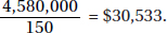
20. (E) The mean, standard deviation, variance, and range are all affected by outliers; the median and interquartile range are not.
21. (C) Because of the squaring operation in the definition, the standard deviation (and also the variance) can be zero only if all the values in the set are equal.
22. (A) The sum of the scores in one class is 20 × 92 = 1840, while the sum in the other is 25 × 83 = 2075. The total sum is 1840 + 2075 = 3915. There are 20 + 25 = 45 students, and
so the average score is 
23. (B) Increasing every value by 5 gives 10% between 45 and 65, and then doubling gives 10% between 90 and 130.
24. (A) 206 + 2.69(35) = 300; 206 – 1.13(35) = 166.
25. (A) Bar charts are used for categorical variables.
26. (C) The median corresponds to the 0.5 cumulative proportion.
27. (A) The 0.25 and 0.75 cumulative proportions correspond to Q1 = 1.8 and Q3 = 2.8, respectively, and so the interquartile range is 2.8 – 1.8 = 1.0.
28. (B) With bell-shaped data the empirical rule applies, giving that the spread from 92 to 98 is roughly 6 standard deviations, and so one SD is about 1.
FREE-RESPONSE
1. (a) Adding 10 to each value increases the mean by 10, but leaves measures of variability unchanged, so the new mean is 340 hours while the range stays at 5835 hours, the standard deviation remains at 245 hours, and the variance remains at 2452 = 60,025 hr2.
(b) Increasing each value by 10% (multiplying by 1.10) will increase the mean to 1.1(330) = 363 hours, the range to 1.1(5835) = 6418.5 hours, the standard deviation to 1.1(245) = 269.5 hours, and the variance to (269.5)2 = 72,630.25 hr2. (Note that the variance increases by a multiple of (1.1)2 not by a multiple of 1.1.)
2. (a) Check for outliers: IQR = 82.6 – 60.4 = 22.2. Q1 – 1.5(IQR) = 27.1 while Q3 + 1.5(IQR) = 115.9, so the only outlier is 26.4.
(b) A complete answer considers shape, center, and spread.
Shape: appears skewed left with an outlier at 26.4
Center: median is 78.0
Spread: from 26.4 to 98.1
(c) When the distribution is skewed left, the mean is usually less than the median.
(d) A stemplot would show more information because it shows all the original data, not just the few values given above; a stemplot can show clusters and gaps which are hidden by a boxplot.
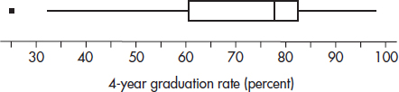
3. (a) The median is 77.5 (millions of dollars), and the IQR = Q3 – Q1 = 159.2 – 33.4 = 125.8 (millions of dollars).
(b) Reducing every value by 3 will reduce the median by 3 but leave measures of variability unchanged, so the new mean is 77.5 – 3 = 74.5 (millions of dollars), and the IQR will still be 125.8 (millions of dollars).
(c) Reducing every value by 50% reduces the median to (0.5)(77.5) = 38.75 (millions of dollars) and reduces the IQR to (0.5)(125.8) = 62.9 (millions of dollars).
(d) The boxplot indicates that the distribution is skewed right, so the mean will be greater than the median. It is unlikely that the two outliers will pull the mean out as far as 325, so the most reasonable value for the mean is 135 (millions of dollars).
4. Z-scores give the number of standard deviations from the mean, so
Q1 = 300 – 0.7(25) = 282.5 and Q3 = 300 + 0.7(25) = 317.5.
The interquartile range is IQR = 317.5 – 282.5 = 35, and 1.5(IQR) = 1.5(35) = 52.5.
The standard definition of outliers encompasses all values less than Q1 – 52.5 = 230 and all values greater than Q3 + 52.5 = 370.
5. (a)
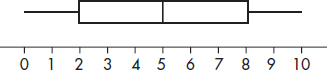
(b) Note that must keep Min = 0, Q1 = 2, Med = 5, Q3 = 8, and Max = 10, with the same totals of in-between values, so move in-between values to the left, and the answer is
{0, 0, 2, 2, 2, 5, 5, 5, 8, 8, 10}.
(c) Note that must keep Min = 0, Q1 = 2, Med = 5, Q3 = 8, and Max = 10, with the same totals of in-between values, so move in-between values outward, and the answer is
{0, 0, 2, 2, 2, 5, 8, 8, 8, 10, 10}.
INVESTIGATIVE TASK
(a) The median of the data values is (48 + 50)/2 = 49.
(b) The absolute deviations from the median are {14, 11, 11, 7, 5, 1, 1, 3, 7, 11, 13, 22}.
In ascending order, these deviations are {1, 1, 3, 5, 7, 7, 11, 11, 11, 13, 14, 22}.
The median of these deviations is MAD = (7 + 11)/2 = 9.
(c) One MAD less than the median is 49 – 9 = 40, and one MAD greater than the median is 49 + 9 = 58. Half of the values (6 values) are between 40 and 58: {42, 44, 48, 50, 52, 56} are all between 40 and 58, whereas half of the values (6 values) are either less than 40 or greater than 58: {35, 38, 38, 60, 62, 71}.
(d) If the top score was 76 rather than 71, the median of the data values would still be 49. The greatest deviation would be 27 rather than 22, but the median deviation would still be 9.
(e) The presence of outliers does not change the value of the MAD (MAD is resistant to outliers). In contrast, the standard deviation (SD) is very sensitive to the presence of outliers (the squares of every deviation from the mean enters the SD calculation).
3 Comparing Distributions
Answers Explained
MULTIPLE-CHOICE
1. (A) The numbers of male and female employees are not given so proportions who are executives cannot be determined.
2. (E) The empirical rule applies to bell-shaped data like those found in set B, not in set A. Both sets are roughly symmetric around 150 and so both should have means about 150. Set A is much more spread out than set B, and so set A has the greater variance. For bell-shaped data, about 95% of the values fall within two standard deviations of the mean and 99.7% fall within three. However, in the histogram for set B, one sees that 95% of the data are not between 140 and 160, and 99.7% are not between 135 and 165. Thus, the standard deviation for set B must be greater than 5.
3. (A) Both sets have 20 elements. The ranges, 76 − 37 = 39 and 86 − 47 = 39, are equal. Brand A clearly has the larger mean and median, and with its skewness it also has the larger variance.
4. (E) The minimum of the combined set of scores must be the min of the boys since it is lower; the maximum of the combined set of scores must be the max of the girls since it is higher; the first quartile must be the same as the identical first quartiles of the two original distributions. There are no outliers (scores more than 1.5(IQR) from the first and third quartiles).
5. (B) Roughly 50% of total bar length is above and below the 15–19 interval.
6. (B) There are about 1.2 million younger than the age of 10 in Liberia (boys and girls) and roughly 3.5 million in Canada.
7. (E) In the Canadian graph, all higher age groups show greater numbers of women than men. In the Liberian graph, the smaller 15–19 age group shows a definite break with the overall pattern (a great number of child soldiers died in the fighting). In the Canadian graph, the narrowing base indicates a decreasing birth rate.
8. (D) The standard deviation is defined in terms of squared deviations from the mean. In the 2014 distribution, more data are concentrated closer to the mean, whereas in the 2015 distribution, more data are further from the mean.
FREE-RESPONSE
1. A complete answer compares shape, center, and spread and mentions context in at least one of the responses.
Shape: The distribution of times to complete all tasks by females is skewed right (toward the higher values), whereas the distributions of times to complete all tasks by males is roughly bell-shaped.
Center: The center of the distribution of female times (at around  minutes) is less than the center of the distribution of male times (at around
  minutes).
Spread: The spreads of the two distributions are roughly the same; the range of the female times ( minutes) equals the range of the male times (
 minutes).
2.
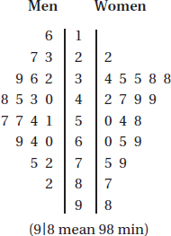
A complete answer compares shape, center, and spread and mentions context in at least one of the responses.
Shape: The men’s distribution of hours grooming is roughly symmetric, whereas the women’s distribution of hours grooming is skewed right (toward higher values).
Center: The center of the men’s distribution is about the same as the center of the women’s distribution, both about 50 min.
Spread: The spread of the men’s distribution (with a range of 82 – 16 = 66 min) is less than the spread of the women’s distribution (with a range of 98 – 22 = 76 min).
3. (a) For females, Q1 – 1.5(IQR) = 130 – 1.5(358 – 130) = –212 and Q3 + 1.5(IQR) = 700, so 1098 is an outlier. For males, Q1 – 1.5(IQR) = 72 – 1.5(273 – 72) = –229.5 and Q3 + 1.5(IQR) = 574.5, so there are no outliers.
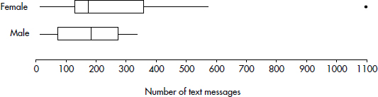
(b) The medians are roughly equal. The male distribution appears roughly symmetric, so the mean is close to the median; however, the female distribution shows extreme right skewness, so the mean is much greater than the median. Thus, the females had a greater mean number of text messages than did the males.
4. A complete answer compares shape, center, and spread and mentions context in at least one of the responses.
Shape: Cruise A, for which the cumulative frequency plot rises steeply at first, has more younger passengers, and thus a distribution skewed to the right (towards the higher ages). Cruise C, for which the cumulative frequency plot rises slowly at first and then steeply towards the end, has more older passengers, and thus a distribution skewed to the left (towards the younger ages). Cruise B, for which the cumulative frequency plot rises slowly at each end and steeply in the middle, has a more bell-shaped distribution.
Center: Considering the center to be a value separating the area under the histogram roughly in half, the centers will correspond to a cumulative frequency of 0.5. Reading across from 0.5 to the intersection of each graph, and then down to the x-axis, shows centers of approximately 18, 40, and 61 years, respectively. Thus, the center of distribution A is the least, and the center of distribution C is the greatest.
Spread: The spreads of the age distributions of all three cruises are the same: from 10 to 70 years.
AN INVESTIGATIVE TASK
(a)
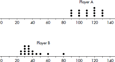
(b) Shape: The Player A distribution is roughly uniform, whereas the Player B distribution is skewed right. (Also, the Player A distribution has no outliers, whereas the Player B distribution looks to have an outlier at 80.)
Center: The center of the Player A distribution (at about 110) is greater than the center of the Player B distribution (at about 35).
Spread: The variability in the Player B distribution is greater than the variability of the Player A distribution (for example, the range in the A distribution is 130 – 90 = 40, whereas the range in the B distribution is 80 – 25 = 55.
(c) The shapes (uniform for A and skewed right for B) are more apparent in the dotplots.
(d) With the dotplots, it’s impossible to see the game to game variability. Also the dotplot for the B distribution doesn’t show the end of year upswing in ratings.
(e) For Player 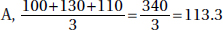 and for Player
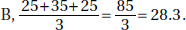
4 Exploring Bivariate Data
Answers Explained
MULTIPLE-CHOICE
1. (E) The variable column indicates the independent (explanatory) variable. The sign of the correlation is the same as the sign of the slope (negative here). In this example, the y-intercept is meaningless (predicted SAT result if no students take the exam). There can be a strong linear relation, with high R2 value, but still a distinct pattern in the residual plot indicating that a non-linear fit may be even stronger. The negative value of the slope (–2.84276) gives that the predicted combined SAT score of a school is 2.84 points lower for each one unit higher in the percentage of students taking the exam, on average.
2. (A) 
3. (D) Residual = Measured – Predicted, so if the residual is negative, the predicted must be greater than the measured (observed).
4. (D) The correlation coefficient is not changed by adding the same number to each value of one of the variables or by multiplying each value of one of the variables by the same positive number.
5. (E) A negative correlation shows a tendency for higher values of one variable to be associated with lower values of the other; however, given any two points, anything is possible.
6. (A) This is the only scatterplot in which the residuals go from positive to negative and back to positive.
7. (E) Since (2, 5) is on the line y = 3x + b, we have 5 = 6 + b and b = –1. Thus the regression line is y = 3x – 1. The point (x, y) is always on the regression line, and so we have y = 3x – 1.
8. (C) The correlation r measures association, not causation.
9. (E) The correlation r cannot take a value greater than 1.
10. (C) If the points lie on a straight line, r = ±1. Correlation has the formula 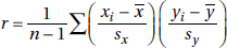 so x and y are interchangeable, and r does not depend on which variable is called x or y. However, since means and standard deviations can be strongly influenced by outliers, r too can be strongly affected by extreme values. While r = 0.75 indicates a better fit with a linear model than r = 0.25 does, we cannot say that the linearity is threefold.
11. (B) The “Predictor” column indicates the independent variable with its coefficient to the right.
12. (E) 
13. (B)  = 0.056 + 0.920 (0.55) = 0.562 and so the residual = 0.59 – 0.562 = 0.028
14. (D) The sum and thus the mean of the residuals are always zero. In a good straight-line fit, the residuals show a random pattern.
15. (C) The coefficient of determination r2 gives the proportion of the y-variance that is predictable from a knowledge of x. In this case r2 = (0.632)2 = 0.399 or 39.9%.
16. (B) The point I doesn’t contribute to a line with negative or positive slope. In none of the scatterplots do the points fall on a straight line, so none of them have correlation 1.0.
17. (C) Predicted winning percentage = 44 + 0.0003(34,000) = 54.2, and
Residual = Observed – Predicted = 55 – 54.2 = 0.8.
18. (B) On each exam, two students had scores of 100. There is a general negative slope to the data showing a moderate negative correlation. The coefficient of determination, r2, is always 0. While several students scored 90 or above on one or the other exam, no student did so on both exams.
19. (E) On the scatterplot all the points lie perfectly on a line sloping up to the right, and so r = 1.
20. (A) The correlation is not changed by adding the same number to every value of one of the variables, by multiplying every value of one of the variables by the same positive number, or by interchanging the x- and y-variables.
21. (B) The slope and the correlation coefficient have the same sign. Multiplying every y-value by –1 changes this sign.
22. (E) A scatterplot readily shows that while the first three points lie on a straight line, the fourth point does not lie on this line. Thus no matter what the fifth point is, all the points cannot lie on a straight line, and so r cannot be 1.
23. (E) All three scatterplots show very strong nonlinear patterns; however, the correlation r measures the strength of only a linear association. Thus r = 0 in the first two scatterplots and is close to 1 in the third.
24. (A) Using your calculator, find the regression line to be  = 9x – 8. The regression line, also called the least squares regression line, minimizes the sum of the squares of the vertical distances between the points and the line. In this case (2, 10), (3, 19), and (4, 28) are on the line, and so the minimum sum is (10 – 11)2 + (19 – 17)2 + (28 – 29)2 = 6.
25. (B) When transforming the variables leads to a linear relationship, the original variables have a nonlinear relationship, their correlation (which measures linearity) is not close to 1, and the residuals do not show a random pattern. While r close to 1 indicates strong association, it does not indicate cause and effect.
26. (E) The least squares line passes through (x, y) = 2,4), and the slope b satisfies
FREE-RESPONSE
1. (a) A calculator gives  12,416 + 180.4 (Wins).
(b) Each additional home win raises the average attendance by about 180 people, on average.
(c) 12,416 + 180.4(25) = 16,926
(d) 17,000 = 12,416 + 180.4(Wins) gives Wins = 25.4 so 26 wins needed to average at least 17,000 average attendance.
(e) With 34 wins, the predicted average attendance is 12,416 + 180.4(34) = 18,550 so the residual is 18,997 – 18,550 = 447.
2. (a)
(b) A calculator gives r = 0.1568.
(c) The correlation r is low for this number of data scores, and the scatterplot shows no linear pattern whatsoever. Although theoretically we could use our techniques to find the best-fitting straight-line approximation, the result would be meaningless and should not be used for predictions.
3. (a) By visual inspection x ≈ 68 and y ≈ 21.
(b) The range of the life expectancies is 80 – 54 = 26, and so the standard deviation is roughly  Similarly the standard deviation of the per capita incomes is roughly
(c) While the points generally fall from the lower left to the upper right, they are still widely scattered. Thus the scatterplot shows a weak positive correlation between per capita income and life expectancy.
4. (a) The correlation for each of the three sets is 0.
(b) The correlation for the set consisting of all 12 scores is 0.9948.
(c) The data from each set taken separately show no linear pattern. However, together they show a strong linear fit. Note the positions of the data from the separate sets in the complete scatterplot.
5. In the first scatterplot, the points fall exactly on a downward sloping straight line, so r = –1. In the second scatterplot, the isolated point is an influential point, and r is close to +1. In the third scatterplot, the isolated point is also influential, and r is close to 0.
6. (a) = –0.16(50) + 34.8 = 26.8 miles per gallon, and = –0.0032(50)2 + 0.258(50) + 23.8 = 28.7 miles per gallon.
(b) Model 2 is the better fit. First, the residuals are much smaller for model 2, indicating that this model gives values much closer to the observed values. Second, a curved residual pattern like that in model 1 indicates that a nonlinear model would be better. A more uniform residual scatter as in model 2 indicates a better fit.
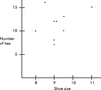
7. (a) The correlation coefficient is 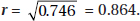 It is positive because the slope of the regression line is positive.
(b) The slope is 1.106, signifying that each additional page raises a grade by 1.106.
(c) Including Mary’s paper will lower the correlation coefficient because her result seems far off the regression line through the other points.
(d) Including Mary’s paper will swing the regression line down and lower the value of the slope.
(e) From the graph, Mary received an 82. From the regression line, Mary would have received = 46.51 + 1.106(45) = 96.3 if she had turned in her paper on time.
8. (a) Yes. The residual graph is not curved, does not show fanning, and appears to be random or scattered.
(b) The slope is 0.95893, indicating that the winning jump improves 0.95893 inches per year on average or about 3.8 inches every four years on average.
(c) With r2 = 0.921, the correlation r is 0.96.
(d) 0.95893(80) + 256.576 ≈ 333.3 inches
(e) The residual for 1980 is +2, and so the actual winning distance must have been 333.3 + 2 = 335.3 inches.
9. (a)
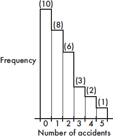
(b)
(c) There is a roughly linear trend with daily accidents increasing during the month.
(d) The daily number of accidents is strongly skewed to the right.
10. (a) The correlation coefficient  It is positive because the slope of the regression line is positive.
(b) The slope is 8.5, signifying that each gram of medication lowers the pulse rate by 8.5 beats per minute.
(c) = –1.68 + 8.5(2.25) = 17.4 beats per minute.
(d) There is always danger in using a regression line to extrapolate beyond the values of x contained in the data. In this case, the 5 grams was an overdose, the patient died, and the regression line cannot be used for such values beyond the data set.
(e) Removing the 3-gram result from the data set will increase the correlation coefficient because the 3-gram result appears to be far off a regression line through the remaining points.
(f) Removing the 3-gram result from the data set will swing the regression line upward so that the slope will increase.
5 Exploring Categorical Data: Frequency Tables
Answers Explained
MULTIPLE-CHOICE
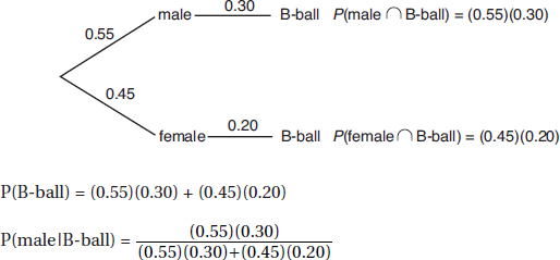
1. (E) Of the 500 people surveyed, 50 + 150 + 50 = 250 were Democrats, and  or 50%.
2. (A) Of the 500 people surveyed, 125 were both for the amendment and Republicans, and 
3. (E) There were 15 + 10 + 25 = 50 Independents; 25 of them had no opinion, and  0.5 or 50%.
4. (E) There were 150 + 50 + 10 = 210 people against the amendment; 150 of them were Democrats, and 
5. (C) The percentages of Democrats, Republicans, and Independents with no opinion are 20%, 12.5%, and 50%, respectively.
6. (A) In the bar corresponding to the Northeast, the segment corresponding to country music stretches from the 50% level to the 70% level, indicating a length of 20%.
7. (B) Based on lengths of indicated segments, the percentage from the West who prefer country is the greatest.
8. (E) The given bar chart shows percentages, not actual numbers.
9. (B) In a complete distribution, the probabilities sum to 1, and the relative frequencies total 100%.
10. (A) The different lengths of corresponding segments show that in different geographic regions different percentages of people prefer each of the music categories.
11. (D) Relative frequencies must be equal. Either looking at rows gives  or looking at columns gives
  We could also set up a proportion
  or
or  Solving any of these equations gives n = 75.
12. (E) It is possible for both to be correct, for example, if there were 11 secretaries (10 women, 3 of whom receive raises, and 1 man who receives a raise) and 11 executives (10 men, 1 of whom receives a raise, and 1 woman who does not receive a raise). Then 100% of the male secretaries receive raises while only 30% of the female secretaries do; and 10% of the male executives receive raises while 0% of the female executives do. However, overall 3 out of 11 women receive raises, while only 2 out of 11 men receive raises. This is an example of Simpson’s paradox.
FREE-RESPONSE
1. (a) i. 
ii. 
iii. 
(b) Calculate row or column totals, and then show either a side-by-side bar graph or a segmented bar graph, showing percentages, and conditioned on either career path (officer vs. enlisted) or military branch:
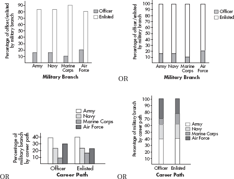
(c) The Army and the Navy have about the same percentage of officers (16%), while the Air Force has a higher percentage of officers (20%), and the Marine Corps has a lower percentage of officers (10%).
OR
Among the officers and the enlisted career paths there are about the same percentage Army (39%), and about the same percentage Navy (23%), while the officers have a lower percentage Marine Corps than the enlisted (9% vs. 16%) and the officers have a higher percentage Air Force than the enlisted (29% vs. 22%).
2. (a)
|
Program |
Percentage of Men Accepted (%) |
Percentage of Women Accepted (%) |
|
A |
62 |
82 |
|
B |
63 |
68 |
|
C |
37 |
34 |
|
D |
33 |
35 |
|
E |
28 |
24 |
|
F |
6 |
7 |
There doesn’t appear to be any real pattern; however, women seem to be favored in four of the programs, while men seem to be slightly favored in the other two programs.
(b) Overall, 1195 out of 2681 male applicants were accepted, for a 45% acceptance rate, while 559 out of 1835 female applicants were accepted, for a 30% acceptance rate. This appears to contradict the results from part a.
(c) You should tell the reporter that while it is true that the overall acceptance rate for women is 30% compared to the 44% acceptance rate for men, program by program women have either higher acceptance rates or only slightly lower acceptance rates than men. The reason behind this apparent paradox is that most men applied to programs A and B, which are easy to get into and have high acceptance rates. However, most women applied to programs C, D, E, and F, which are much harder to get into and have low acceptance rates.
6 Overview of Methods of Data Collection
Answers Explained
MULTIPLE-CHOICE
1. (C) This study is not an experiment in which responses are being compared. It is an observational study in which the airlines use split fare calculations from a trial period as a sample to indicate the pattern of all split fare transactions. A census listing all possible connecting flights was not attempted.
2. (E) The first two sentences can be considered part of the definitions of experiment and observational study. A sample survey does not impose any treatment; it simply counts a certain outcome, and so it is an observational study, not an experiment. A complete census can provide much information about a population, but it doesn’t necessarily establish a cause-and-effect relationship among seemingly related population parameters.
3. (B) The first study was observational because the subjects were not chosen for treatment.
4. (A) The first study was an experiment with two treatment groups and no control group. The second study was observational; the researcher did not randomly divide the subjects into groups and have each group sleep a designated number of hours per night.
5. (E) This study was an experiment in which the researchers divided the subjects into treatment and control groups. A census would involve a study of all migraine sufferers, not a sample of 20. The response of the treatment group receiving chocolate was compared to the response of the control group receiving a placebo. The peppermint tablet with no chocolate was the placebo.
6. (A) The main office at your school should be able to give you the class sizes of every math and English class. If need be, you can check with every math and English teacher.
7. (C) In the first study the families were already in the housing units, while in the second study one of two treatments was applied to each family.
8. (E) Both studies apply treatments and measure responses, and so both are experiments.
7 Planning and Conducting Surveys
Answers Explained
MULTIPLE-CHOICE
1. (A) This survey provides a good example of voluntary response bias, which often overrepresents negative opinions. The people who chose to respond were most likely parents who were very unhappy, and so there is very little chance that the 10,000 respondents were representative of the population. Knowing more about her readers, or taking a sample of the sample would not have helped.
2. (D) If there is bias, taking a larger sample just magnifies the bias on a larger scale. If there is enough bias, the sample can be worthless. Even when the subjects are chosen randomly, there can be bias due, for example, to non-response or to the wording of the questions. Convenience samples, like shopping mall surveys, are based on choosing individuals who are easy to reach, and they typically miss a large segment of the population. Voluntary response samples, like radio call-in surveys, are based on individuals who offer to participate, and they typically overrepresent persons with strong opinions.
3. (E) The wording of the questions can lead to response bias. The neutral way of asking this question would simply have been: Are you in favor of a 7-day waiting period between the filing of an application to purchase a handgun and the resulting sale?
4. (E) In a simple random sample, every possible group of the given size has to be equally likely to be selected, and this is not true here. For example, with this procedure it will be impossible for all the Bulls to be together in the final sample. This procedure is an example of stratified sampling, but stratified sampling does not result in simple random samples.
5. (E) In a simple random sample, every possible group of the given size has to be equally likely to be selected, and this is not true here. For example, with this procedure it will be impossible for all the early arrivals to be together in the final sample. This procedure is an example of systematic sampling, but systematic sampling does not result in simple random samples.
6. (B) Different samples give different sample statistics, all of which are estimates of a population parameter. Sampling error relates to natural variation between samples, can never be eliminated, can be described using probability, and is generally smaller if the sample size is larger.
7. (B) The Wall Street Journal survey has strong selection bias; that is, people who read the Journal are not very representative of the general population. The talk show survey results in a voluntary response sample, which typically gives too much emphasis to persons with strong opinions. The police detective’s survey has strong response bias in that students may not give truthful responses to a police detective about their illegal drug use.
8. (E) While the auditor does use chance, each company will have the same chance of being audited only if the same number of companies have names starting with each letter of the alphabet. This will not result in a simple random sample because each possible set of 26 companies does not have the same chance of being picked as the sample. For example, a group of companies whose names all start with A will not be chosen. Calculator random number generators and random number tables have similar uses and results.
9. (D) This is not a simple random sample because all possible sets of the required size do not have the same chance of being picked. For example, a set of households all from just half the counties has no chance of being picked to be the sample. Stratified samples are often easier and less costly to obtain and also make comparative data available. In this case responses can be compared among various counties. There is no reason to assume that each county has heads of households with the same characteristics and opinions as the state as a whole, so cluster sampling is not appropriate. When conducting stratified sampling, proportional sampling is used when one wants to take into account the different sizes of the strata.
10. (C) It is most likely that the apartments at which the interviewer had difficulty finding someone home were apartments with fewer students living in them. Replacing these with other randomly picked apartments most likely replaces smaller-occupancy apartments with larger-occupancy ones.
11. (E) While the procedure does use some element of chance, all possible groups of size 50 do not have the same chance of being picked, and so the result is not a simple random sample. There is a very real chance of selection bias. For example, a number of relatives with the same name and similar long-distance calling patterns might be selected. The typical methodology of a systematic sample involves picking every nth member from the list, where n is roughly the population size divided by the desired sample size.
12. (A) The natural variation in samples is called sampling error. Embarrassing questions and resulting untruthful answers are an example of response bias. Inaccuracies and mistakes due to human error are one of the real concerns of researchers.
13. (C) Surveying people coming out of any church results in a very unrepresentative sample of the adult population, especially given the question under consideration. Using chance and obtaining a high response rate will not change the selection bias and make this into a well-designed survey.
Free-Response
1. (a) Both studies were observational because no treatments were applied.
(b) Typical cell phone use today, especially among younger people, is well over half an hour, so half an hour does not seem to be a reasonable split between moderate and heavy use.
(c) This absolutely affects conclusions in that both studies look for relationships with brain cancer. While voice conversation involves holding the phone against one’s head, text messaging does not.
(d) The Denmark study looks at how many years individuals used their cell phones, but not at the extent of daily use, while the WHO study does consider daily usage.
2. There are many possible examples, such as Are you in favor of protecting the habitat of the spotted owl, which is almost extinct and desperately in need of help from an environmentally conscious government? and Are you in favor of protecting the habitat of the spotted owl no matter how much unemployment and resulting poverty this causes among hard-working loggers?
3. (a) To be a simple random sample, every possible group of size 25 has to be equally likely to be selected, and this is not true here. For example, if there are 40 students who always rush to be first in line, this procedure will allow for only 2 of them to be in the sample. Or if each homeroom of size 20 arrives as a unit, this procedure will allow for only 1 person from each homeroom to be in the sample.
(b) A simple random sample of the students can be obtained by numbering them from 001 to 500 and then picking three digits at a time from a random number table, ignoring numbers over 500 and ignoring repeats, until a group of 25 numbers is obtained. The students corresponding to these 25 numbers will be a simple random sample.
4. The direct telephone and mailing options will both suffer from undercoverage bias. For example, especially affected by the legislation under discussion are the homeless, and they do not have telephones or mailing addresses. The pollster interviews will result in a convenience sample, which can be highly unrepresentative of the population. In this case, there might be a real question concerning which members of her constituency spend any time in the downtown area where her office is located. The radio appeal will lead to a voluntary response sample, which typically gives too much emphasis to persons with strong opinions.
5. In numbering the people 0 through 9, each digit stands for whose coat someone receives. Pick the digits, omitting repeats, until a group of ten different digits is obtained. Check for a match (1 appearing in the first position corresponding to person 1, or 2 appearing in the next position corresponding to person 2, and so on, up to 0 appearing in the last position corresponding to person 10).
6. (a) To obtain an SRS, you might use a random number table and note the first two different numbers between 1 and 5 that appear. Or you could use a calculator to generate numbers between 1 and 5, again noting the first two different numbers that result.
(b) Time and cost considerations would be the benefit of substitution. However, substitution rather than returning to the same home later could lead to selection bias because certain types of people are not and will not be home at 9 a.m. With substitution the sample would no longer be a simple random sample.
(c) Corner lot homes like homes 1 and 5 might have different residents (perhaps with higher income levels) than other homes.
7. (a) Method A is an example of cluster sampling, where the population is divided into heterogeneous groups called clusters and individuals from a random sample of the clusters are surveyed. It is often more practical to simply survey individuals from a random sample of clusters (in this case, a random sample of city blocks) than to try to randomly sample a whole population (in this case the entire city population).
(b) Method B is an example of stratified sampling, where the population is divided into homogeneous groups called strata and random individuals from each stratum are chosen. Stratified samples can often give useful information about each stratum (in this case, about each of the five neighborhoods) in addition to information about the whole population (the city population).
AN INVESTIGATIVE TASK
(a) 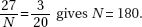 gives N = 180.
(b) 
(c) No, this would not have been unexpected because 45, the absolute difference between 180 and 225, is less than the standard deviation of 54.76.
(d) 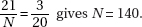
8 Planning and Conducting Experiments
Answers Explained
MULTIPLE-CHOICE
1. (D) It may well be that very bright students are the same ones who both take AP Statistics and have high college GPAs. If students could be randomly assigned to take or not take AP Statistics, the results would be more meaningful. Of course, ethical considerations might make it impossible to isolate the confounding variable in this way. Only using a sample from the observations gives less information.
2. (B) The desire of the workers for the study to be successful led to a placebo effect.
3. (C) In experiments on people, the subjects can be used as their own controls, with responses noted before and after the treatment. However, with such designs there is always the danger of a placebo effect. Thus the design of choice would involve a separate control group to be used for comparison.
4. (B) Blocking divides the subjects into groups, such as men and women, or political affiliations, and thus reduces variation.
5. (D) Blocking in experiment design first divides the subjects into representative groups called blocks, just as stratification in sampling design first divides the population into representative groups called strata. This procedure can control certain variables by bringing them directly into the picture, and thus conclusions are more specific. The paired comparison design is a special case of blocking in which each pair can be considered a block. Unnecessary blocking detracts from accuracy because of smaller sample sizes.
6. (E) None of the studies has any controls, such as randomization, control groups, or blinding, and so while they may give valuable information, they cannot establish cause and effect.
7. (D) Octane is the only explanatory variable, and it is being tested at four levels. Miles per gallon is the single response variable.
8. (A) There is nothing wrong with using volunteers—what is important is to randomly assign the volunteers into the two treatment groups. There is no way to use blinding in this study—the subjects will clearly know which breakfast they are eating. The main idea behind randomly assigning subjects to the different treatments is to control for various possible confounding variables—it is reasonable to assume that people of various ages, races, ethnic backgrounds, etc., are assigned to receive each of the treatments.
9. (E) In good observational studies, the responses are not influenced during the collecting of data. In good experiments, treatments are compared as to differences in responses. In an experiment, there can be many treatments, each at a different level. Well-designed experiments can show cause and effect.
10. (D) Control, randomization, and replication are all important aspects of well-designed experiments. Care in observing without imposing change refers to observational studies, not experiments.
11. (A) Each subject might receive both treatments, as, for example, in the Pepsi-Coke taste comparison study. The point is to give each subject in a matched pair a different treatment and note any difference in responses. Matched-pair experiments are a particular example of blocking, not vice versa. Stratification refers to a sampling method, not to experimental design. Randomization is used to decide which of a pair gets which treatment or which treatment is given first if one subject is to receive both.
12. (A) Blinding does have to do with whether or not the subjects know which treatment (color in this experiment) they are receiving. However, drinking out of solid colored thermoses makes no sense since the beverages are identical except for color and the point of the experiment is the teenager’s reaction to color. Blinding has nothing to do with blocking (team participation in this experiment).
13. (A) This study is an experiment because a treatment (periodic removal of a pint of blood) is imposed. There is no blinding because the subjects clearly know whether or not they are giving blood. There is no blocking because the subjects are not divided into blocks before random assignment to treatments. For example, blocking would have been used if the subjects had been separated by gender or age before random assignment to give or not give blood donations. There is a single factor—giving or not giving blood.
FREE-RESPONSE
1. (a) These are observational studies as there is no randomization of treatments to subjects.
(b) The excitement of a birthday party is a confounding variable. Without conducting a proper experiment, there is no way of telling whether observed hyperactivity is caused by sugar or by the excitement of a party or by some other variable.
(c) The parent should randomly give the child sugar or sugar-free sweets at parties and observe the child’s behavior. It is important that the parent not know which the child is receiving (double blinding), because the parent might perceive a difference in behavior which is not really there if he/she knows whether or not the child is being given a sugary food.
2. Ask doctors, hospitals, or blood testing laboratories to make known that you are looking for HIV-positive volunteers. As the volunteers arrive, use a random number table to give each one the drug or a placebo (e.g., if the next digit in the table is odd, the volunteer gets the drug, while if the next digit is even, the volunteer gets a placebo). Use double-blinding; that is, both the volunteers and their doctors should not know if they are receiving the drug or the placebo. Ethical considerations will arise, for example, if the drug is very successful. If volunteers on the placebo are steadily developing full-blown AIDS while no one on the drug is, then ethically the test should be stopped and everyone put on the drug. Or if most of the volunteers on the drug are dying from an unexpected fatal side effect, the test should be stopped and everyone taken off the drug.
TIP
Simply saying to “randomly assign” subjects to treatment groups is usually an incomplete response. You need to explain how to make the assignments—for example, by using a random number table or through generating random numbers on a calculator.
3. To achieve blocking by gender, first separate the men and women. Label the 40 men 01 through 40. Use a random number table to pick two digits at a time, ignoring 00 and numbers greater than 40, and ignoring repeats, until a group of ten such numbers is obtained. These men will receive the supplement at the once-a-day level. Follow along in the table, continuing to ignore repeats, until another group of ten is selected. These men will receive the supplement at the twice-a-day level. Again ignore repeats until a third group of ten is selected to receive the supplement at the three-times-a-day level, while the remaining men will be a control group and not receive the supplement. Now repeat the entire procedure, starting by labeling the women 01 through 40. A decision should be made whether or not to use a placebo and have all participants take “something” three times a day. Weigh all 80 overweight volunteers before and after a predetermined length of time. Calculate the change in weight for each individual. Calculate the average change in weight among the ten people in each of the eight groups. Compare the four averages from each block (men and women) to determine the effect, if any, of different levels of the supplement for men and for women.
4. The first study, an observational study, does not suffer from nonresponse bias, as do most mailed questionnaires, because it involved follow-up telephone calls and achieved a high response rate. However, this study suffers terribly from selection bias because people who subscribe to a health magazine are not representative of the general population. One would expect most of them to strongly believe that vitamins improve their health. The second study, a controlled experiment, used comparison between a treatment group and a control group, used randomization in selecting who went into each group, and used blinding to control for a placebo effect on the part of the volunteers. However, it did not use double-blinding; that is, the doctors knew whether their patients were receiving the vitamin, and this could have introduced hidden bias when they made judgments regarding their patients’ health.
5. Every day for some specified period of time, look at the next digit on a random number table. If it is odd, flash the subliminal message all day on the screen, while if it is even, don’t flash the message that day (randomization). Don’t let the customers know what is happening (blinding) and don’t let the clerks selling the popcorn know what is happening (double-blinding). Compare the quantity of popcorn bought by the treatment group, that is, by the people who receive the subliminal message, to the quantity bought by the control group, the people who don’t receive the message (comparison).
6. Any conclusions would probably be meaningless. There is a substantial danger of the placebo effect here; that is, real physical responses could be caused by the psychological effect of knowing the intent of the research. The experiment would be considerably strengthened by using a control group taking a look-alike capsule. Any conclusions are further suspect because of the choice of subjects. Rather than making a random selection from the intended population, the company is using a sample from its own employees, a sample almost guaranteed to have concerns, interests, and backgrounds that will confound the responses or limit their generalizability.
7. Ask doctors and hospitals to make known that you are looking for volunteers from among intractable pain sufferers. As the volunteers arrive, use a random number table to decide which will have the electrodes properly embedded in their pain centers and which will have the electrodes harmlessly embedded in wrong positions. For example, if the next digit in the table is odd, the volunteer receives the proper embedding, while if the next digit is even, the volunteer does not. Use double-blinding; that is, both the volunteers and their doctors should not know if the volunteers are receiving the proper embedding. Ethical considerations will arise, for example, if the procedure is very successful. If volunteers with the wrong embeddings are in constant pain, while everyone with proper embedding is pain-free, then ethically the test should be stopped and everyone given the proper embedding. Or if most of the volunteers with proper embedding develop an unexpected side effect of the pain spreading to several nearby sites, then the test should be stopped and the procedure discontinued for everyone.
8. To achieve blocking by sunlight, first separate the sunlit and shaded plots. Label the 15 sunlit plots 01 through 15. Using a random number table, pick two digits at a time, ignoring 00 and numbers above 15 and ignoring repeats, until a group of five such numbers is obtained. These sunlit plots will receive the fertilizer at regular concentration. Continue in the table, ignoring repeats, until another group of five is selected. These sunlit plots will receive the fertilizer at double concentration, while the remaining sunlit plots will be a control group receiving no fertilizer. Now repeat the procedure, this time labeling the shaded plots 01 through 15. Assuming size is the pertinent outcome, weigh all vegetables at the end of the season, compare the average weights among the three sunlit groups, and compare the average weights among the three shaded groups to determine the effect of the fertilizer, if any, at different levels on sunlit plots and separately on shaded plots.
9. The first study, an observational study, does not suffer from nonresponse bias, as do most studies involving mailed questionnaires, because the researchers made follow-up telephone calls and achieved a very high response rate. However, the first study suffers terribly from selection bias. People who work at a teaching hospital are not representative of the general population. One would expect many of them to have heard about how zinc coats the throat to hinder the propagation of viruses. The second study, a controlled experiment, used comparison between a treatment group and a control group, used randomization in selecting who went into each group, and used blinding to control for a placebo effect on the part of the volunteers. However, they did not use double-blinding; that is, the doctors knew whether their patients were receiving the zinc lozenges, and this could introduce hidden bias as the doctors make judgments about their patients’ health.
10. For each new heart attack patient entering the hospital, look at the next digit from a random number table. If it is odd, give the name to a group of people who will pray for the patient throughout his or her hospitalization, while if it is even, don’t ask the group to pray (randomization). Don’t let the patients know what is happening (blinding) and don’t let the doctors know what is happening (double-blinding). Compare the lengths of hospitalization of patients who receive prayers with those of control group patients who don’t receive prayers (comparison).
11. (a) Allowing the students to self-select which class to take leads to confounding that could be significant. For example, perhaps the brighter students all want to learn a certain one of the three languages.
(b) It is possible for the average score of all science majors to be lower than the average for all math majors even though the science majors averaged higher in each class. For example, suppose that the students taking Java scored much higher than the students in the other two classes. Furthermore, only one science major took Java, and she scored tops in the class. Then the overall average of the math majors could well be higher. This is an example of Simpson’s paradox, in which a comparison can be reversed when more than one group is combined to form a single group.
(c) Number the students 001 through 300. Read off three digits at a time from a random number table, noting all triplets between 001 and 300 and ignoring repeats, until 100 such numbers have been selected. Keep reading off three digits, ignoring repeats, until 100 new numbers between 001 and 300 are selected. These get C++, while the remaining 100 get Java. Even quicker would be to use a calculator to generate random digits between 001 and 300.
(d) Go through the list of students, flipping a die for each. If a 1 or a 2 shows, the student takes Pascal, if a 3 or a 4 shows, C++, and if a 5 or a 6 shows, Java.
(e) Another possible variable are the teachers. For example, perhaps the better teachers teach Java.
AN INVESTIGATIVE TASK
(a) There is no reason to believe that there was anything random about which students took which course. Perhaps all the weaker students self-selected or were advised to choose the traditional course.
(b) The students could be labeled 01 through 50. Pairs of digits could then be read off a random number table, ignoring numbers over 50 and ignoring duplicates, until a set of 25 numbers is obtained. The students corresponding to these numbers could be enrolled in the traditional course, and the remaining students in the other.
(c) Applying the above procedure results in {17, 31, 14, 35, 41, 05, 09, 20, 06, 44, 50, 43, 11, 18, 45, 01, 13, 33, 04, 19, 02, 08, 40, 49, 03}. Enroll the students with these numbers in the traditional course.
(d) Which teachers teach which courses is not considered. Perhaps the more interesting, exciting teachers teach the new version. Even though a control group is selected, there is no blinding, and so students in the new version might work harder because they realize they are part of an experiment.
9 Probability as Relative Frequency
Answers Explained
MULTIPLE-CHOICE
1. (E) There is no reason to assume that the probability of getting a 5 is the same as that of not getting a 5.
2. (E) The probability that both events will occur is the product of their separate probabilities only if the events are independent, that is, only if the chance that one event will happen is not influenced by whether or not the second event happens. In this case the probability of different surgeries failing are probably closely related.
3. (B) P(1st die is 4)P(2nd die is 6) + P(1st die is 6)P(2nd die is 4) + P(1st die is 5)P(2nd die is 5)
4. (A) 10(0.15)2(0.85)3 = 0.138 or binompdf(5, .15, 2) = 0.138
5. (B) The probability of the next child being a girl is independent of the gender of the previous children.
6. (B) 1 – (0.99975)100 = 0.0247
7. (D) 0.001(1,500,000) = 1500
8. (D) 

[Or on the TI-84, put returns and probabilities into two lists and run 1-Var Stats L1,L2]
9. (C)  are honors students, and
  prefer basketball. Because of independence, their intersection is (0.25)(0.3) = 0.075 of the students, and 0.075(6000) = 450.
10. (E) (0.9)3 + 3(0.9)2(0.1) = 0.972
11. (D) 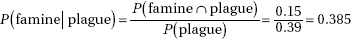
12. (B) If E and F are independent, then P(E  F) = P(E)P(F); however, in this problem, (0.4)(0.35) ≠ 0.3.
13. (B) Because A and B are independent, we have P(A B) = P(A)P(B), and thus P(A ∪ B) = 0.2 + 0.1 – (0.2)(0.1) = 0.28.
14. (D) 
15. (B) E(X) = µx = xipi = 700(0.05) + 540(0.25) + 260(0.7) = 352
16. (D) The probability of throwing heads is 0.5. By the law of large numbers, the more times you flip the coin, the more the relative frequency tends to become closer to this probability. With fewer tosses there is a greater chance of wide swings in the relative frequency.
17. (E) P(diamond on 2nd pick) = 1/4; however,
P(diamond on 2nd pick | heart on first pick) = 13/51
P(black on 2nd pick) = 1/2; however, P(black on 2nd pick | red on 1st pick) = 26/51
P(ace on 2nd pick) = 1/13; however, P(ace on 2nd pick | ace on 1st pick) = 3/51
P(two kings) = (1/13)(3/51); however, P(two kings | two aces) = 0
P(black on 2nd pick) = 1/2 and P(black on 2nd pick | two aces) = 6/12
18. (B) P(two kings) = (1/13)(1/13); however, P(two kings | two aces) = 0
P(king on 2nd pick) = 1/13, and P(king on 2nd pick | ace on 1st pick) = 1/13
P(at least one king) = 1 – (12/13)2 = 25/169; however,
P(at least one king | at least one ace) = [(1/13)(1/13) + (1/13)(1/13)]/[25/169] = 2/25
P(exactly one king) = (1/13)(12/13) + (12/13)(1/13) = 24/169; however,
P(exactly one king | exactly one ace) = (2/169)/(24/169) = 1/12
P(no kings) = (12/13)2; however, P(no kings | no aces) = (11/12)2
19. (A) E(X) = µx = xipi = 21,000(0.8) + 35,000(0.2) = 23,800
20. (D) 1000(0.2) + 5000(0.05) = 450, and 800 – 450 = 350.
21. (E) 
22. (D) P(E F) = P(E)P(F) only if the events are independent. In this case, women live longer than men and so the events are not independent.
For Questions 23–27, we first sum the rows and columns:
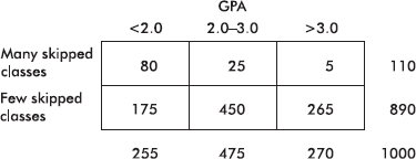
23. (D) 
24. (A)  (probability of an intersection)
25. (C)  (probability of a union)
26. (E) 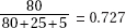 (conditional probability)
27. (A)  0.506. If independent, these would have been equal.
28. (E) While the outcome of any single play on a roulette wheel or the age at death of any particular person is uncertain, the law of large numbers gives that the relative frequencies of specific outcomes in the long run tend to become closer to numbers called probabilities.
29. (D) 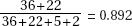
30. (A) 
31. (A) 
32. (E) 
33. (E) 
34. (B)
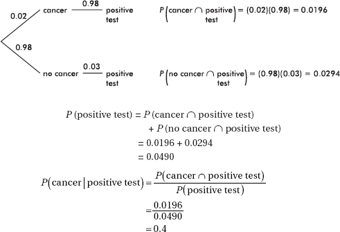
35. (D) The probability that you will receive an A in AP Statistics but not in AP Biology must be 0.35 – 0.19 = 0.16, not 0.17.
36. (B) Your expected winnings are only

37. (C) Even though the first two choices have a higher expected value than the third choice, the third choice gives a 100% chance of avoiding bankruptcy.
38. (A) The probabilities  are all nonnegative, and they sum to 1.
39. (D) 6(0.65)2(0.35)2 = 0.311 or binompdf(4, .65, 2) = 0.311
40. (C) This is a binomial with n = 10 and p = 0.37, and so the mean is np = 10(0.37) = 3.7.
41. (D) 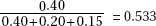
42. (E) Coins have no memory, and so the probability that the next toss will be heads is .5 and the probability that it will be tails is 0.5. The law of large numbers says that as the number of tosses becomes larger, the percentage of heads tends to become closer to 0.5.
43. (B) The probabilites of each pump not failing are 1 – 0.025 = 0.975, 1 – 0.034 = 0.966, and 1 – 0.02 = 0.98, respectively. The probability of none failing is (0.975)(0.966)(0.98) = .923, and so the probability of at least one failing is 1 – 0.923 = 0.077.
44. (B) If p > 0.5, the more likely numbers of successes are to the right and the lower numbers of successes have small probabilities, and so the histogram is skewed to the left. No matter what p is, if n is sufficiently large, the histogram will look almost symmetric.
45. (B)
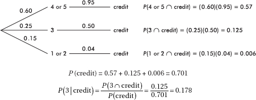
46. (B) If A and B are mutually exclusive, P(A B) = 0. Thus 0.6 = 0.4 + P(B) – 0, and so P(B) = 0.2. If A and B are independent, then P(A B) = P(A)P(B). Thus 0.6 = 0.4 + P(B) – 0.4P(B), and so P(B) = 
47. (A) For each of the 20 students, we must generate an answer to each of the 10 questions, and record if any student has at least 6 out of 10 correct answers.
FREE-RESPONSE
1. With Option A, if in reality only 75% of the articles meet all specifications, the probability of rejecting the day’s production is:

[On the TI-84, binomcdf(6,.75,4) = .466]
With Option B, if in reality only 75% of the articles meet all specifications, the probability of rejecting the day’s production is:
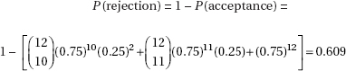
[On the TI-84, binomcdf(12,.75,9) = .609]
For the greatest probability of rejecting the day’s production if only 75% of the articles meet all specifications, the buyer should request the manufacturer to use Option B with a probability of rejection of 0.609 as opposed to Option A with a probability of rejection of only 0.466.
2. It’s easiest to first sum the rows and columns:
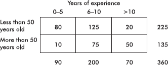
(a) 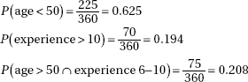
(b) 
(c) 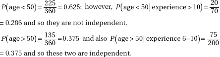
3. If USAir accounted for 20% of the major disasters, the chance that it would be involved in at least four of seven such disasters is
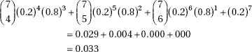
[Or binomcdf(7, .8, 3) = 0.033.]
Mathematically, if USAir accounted for only 20% of the major disasters, there is only a 0.033 chance of it being involved in four of seven such disasters. This seems more than enough evidence to be suspicious!
4.
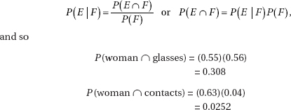
If 55% of those who wear glasses are women, 45% of those who wear glasses must be men, and if 63% of those who wear contacts are women, 37% of those who wear contacts must be men. Thus we have
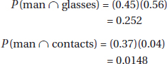
The probability that you will encounter a person not wearing glasses or contacts is 1 – (0.308 + 0.0252 + 0.252 + 0.0148) = 0.4.
5. (a) The probability of the complement is 1 minus the probability of the event, but 1 – 0.43 ≠ 0.47.
(b) Probabilities are never greater than 1, but 6(0.18) = 1.08.
(c) The probability of an intersection cannot be greater than the probability of one of the separate events.
(d) The probability of a union cannot be less than the probability of one of the separate events.
(e) Probabilities are never negative.
6. (a) Player B wins only if both a 10 shows on the coin (a probability of  ) and a 7 shows on the die (a probability of
  ). These events will both happen
  of the time, and so player A wins of the time or twice as often as player B. Thus, to make this a fair game, player B should receive $0.50 each time he wins.
TIP
When using a formula, write down the formula and then substitute the values.
(b) Player A’s expected payoff is
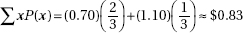
while player B’s expected payoff is
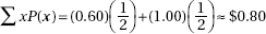
7. (a) We have a binomial with n = 20 and p = 0.15, so

[The answer comes quickly from a calculator calculation such as 1-binomcdf(20, .15, 9) on the TI-84.]
(b) If the probability of Legionella bacteria growing in an electric faucet is 0.15, then the probability of a result as extreme or more extreme than what was obtained in the Johns Hopkins study is only 0.00025. With such a low probability, there is strong evidence to conclude that the probability of Legionella bacteria growing in electronic faucets is greater than .15. That is, there is strong evidence that automatic faucets actually house more bacteria than the old-fashioned, manual kind!
INVESTIGATIVE TASK
(a) Let the numbers 01 through 14 represent finding an illegal drug, while 15 through 99 and 00 represent no drugs. Read off pairs of digits from the random number table until a number representing illegal drugs is found or until nine clean cars are allowed to pass. Note whether a car with illegal drugs is found before nine clean cars pass. Repeat this procedure. Underlining numbers representing the presence of illegal drugs gives
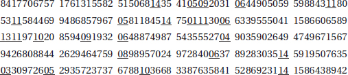
The first nine cars are clean. Then 14 is found after four clean cars, then 05 after two clean cars, then 09 before any clean cars, then 06 after two clean cars, then 11 after seven free cars, and so on. Tabulating gives
First nine cars clean: 5
Illegal drugs found before tenth car: 24
The probability that illegal drugs will be found before the tenth car is estimated to be 
(b) xP(x) = 1(0.15) + 2(0.12) + · · · + 25(0.01) = 6.81
(c) The probability that the first stopped car will have illegal drugs is 0.14. The probability that the first will be clean but that the second will have drugs is (0.86)(0.14). The probability that two clean cars will be followed by one with drugs is (0.86)2(0.14). The probability that three clean ones will be followed by one with drugs is (0.86)3(0.14), and so on. The probability of drugs being found before the tenth car is
0.14 + (0.86)(0.14) + (0.86)2(0.14) + · · · + (0.86)8(0.14) = 0.7427
Or more simply we could solve by subtracting the complementary probability from 1, that is, 1 – (0.86)9 = 0.7427.
10 Combining Independent Random Variables
Answers Explained
MULTIPLE-CHOICE
1. (D) Expected values and variances add. Thus,
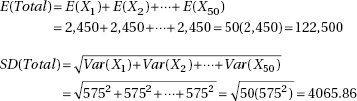
2. (C) For a set of differences, means subtract, but variances add. Thus,

3. (B) Expected values and variances add. Thus,
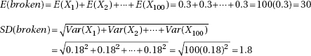
4. (C) For a set of differences, means subtract, but variances add. Thus,
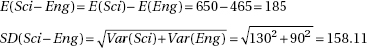
5. (C) Means and variances add. Thus,
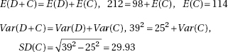
6. (A) Means and variances add. Thus,
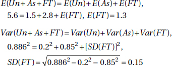
7. (B) Means and variances add. Thus,
E(Total )= E(Box)+50E(Hole), 16.0 = 1.0+50E(Hole), E(Hole)= 0.3
Var(Total) = Var(Box) + 50Var(Hole),
0.2452 = 0.22 + 50(SD(Hole))2, SD(Hole) = 0.02
AN INVESTIGATIVE TASK
(a) 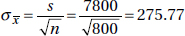
(b) 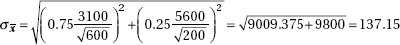
(c) The means for each school type are significantly different, and the variability around the mean for each separate school type is much less than what it was for the first researcher. The second researcher took advantage of this decreased variability within school types, whereas the first researcher has more variability because all the bachelor’s degree recipients are put together in a single sample.
11 The Normal Distribution
Answers Explained
MULTIPLE-CHOICE
1. (A) The area under any probability distribution is equal to 1. Many bell-shaped curves are not normal curves. The smaller the standard deviation of a normal curve, the higher and narrower the graph. The mean determines the value around which the curve is centered; different means give different centers. Because of symmetry, the mean and median are identical for normal distributions.
2. (B) Statement (B) is true by symmetry of the normal curve, however 0.4772 is not twice 0.3413, 0.67 – (–0.67) is not 3, the range is not finite, and the P(z < 0.1) is more than 0.5 while P(z > 0.9) is less than 0.5.
3. (E) All normal distributions have about 95% of their observations within two standard deviations of the mean.
4. (C) Curve a has mean 6 and standard deviation 2, while curve b has mean 18 and standard deviation 1.
5. (B) The z-score of 10 is  From Table A, to the left of –2 is an area of
0.0228. [normalcdf(0, 10, 12.4, 1.2) = 0.0228.]
6. (A) The z-score of 3 is  From Table A, to the left of 0.65 is an area of 0.7422, and so to the right must be 1 – 0.7422 = 0.2578. [normalcdf(3, 1000, 2.43, .88) = 0.2589.]
7. (E) The z-scores of 3 and 4 are 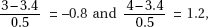 respectively. From Table A, to the left of –0.8 is an area of 0.2119, and to the left of 1.2 is an area of 0.8849. Thus between 3 and 4 is an area of 0.8849 – 0.2119 = 0.6730. [normalcdf(3, 4, 3.4, .5) = 0.6731.]
8. (B) If 95% of the area is to the right of a score, 5% is to the left. Looking for 0.05 in the body of Table A, we note the z-score of –1.645. Converting this to a raw score gives 500 – 1.645(100) = 336. [invNorm(.05, 500, 100) = 336.]
9. (E) The critical z-score associated with 99% to the left is 2.326, and 30 + 2.326(4) = 39.3. [invNorm(.99, 30, 4) = 39.3.]
10. (B) The critical z-scores associated with the middle 95% are ±1.96, and 9500 ± 1.96(1750) = 6070 and 12,930. [invNorm(.025, 9500, 1750) = 6070 and invNorm(.975, 9500, 1750) = 12,930.]
11. (B) 
12. (A) The critical z-score associated with 18% to the right or 82% to the left is 0.92. Then 100 + 0.92 = 120 gives = 21.7.
13. (A) The critical z-score associated with 85% to the left is 1.04. Then µ + 1.04(2) = 16 gives µ = 13.92.
14. (D) The critical z-scores associated with 75% to the right (25% to the left) and with 15% to the right (85% to the left) are –0.67 and 1.04, respectively. Then {µ – 0.67 = 75, µ + 1.04 = 150} gives µ = 104.39 and = 43.86.
15. (A) The critical z-score associated with 0.5% to the right (99.5% to the left) is 2.576. Then c + 2.576(0.4) = 8 gives c = 6.97.
16. (A) Using the normal as an approximation to the binomial, we have µ = 30(0.5) = 15, 2 = 30(0.5)(0.5) = 7.5, = 2.739,  = 1.64, and 1 – 0.9495 = 0.0505. [Or binomcdf(30, .5, 10) = 0.0494.]
17. (A) The critical z-scores for 10% to the left and 5% to the right are –1.282 and 1.645, respectively. Then {µ – 1.282 = 2.48, µ + 1.645 = 2.54} gives µ = 2.506 and = 0.0205.
FREE-RESPONSE
1. (a) Let the random variable D be the difference in walking times (Steve–Jan). Then µD = 30 – 25 = 5 and 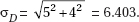 For Steve to arrive before Jan, the difference in walking times must be < 0.
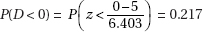
(b) If m is the number of minutes he should leave early, then the new mean of the differences is 5 – m, and we want 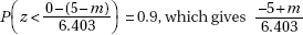 and m = 13.2 minutes.
2. (a) 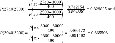
Given independence, the probability that both components last 240 more hours is (0.829825)(0.665506) = 0.552.
(b) The probability that both fail is (1 – 0.829825)(1 – 0.665506) = 0.056923.
The probability that at least one doesn’t fail is 1 – 0.056923 ≈ 0.943.
INVESTIGATIVE TASKS
1. (a) The announcer meant that to maintain his tabulated free throw percentage, Jordan would have to soon miss one. This is not a correct use of probability. If Jordan makes a certain percentage of free throws, that probability applies to each throw irrespective of the previous throws. By the law of large numbers, in the long run the relative frequency tends toward the correct probability, but no conclusion is possible about any given outcome.
(b) P(six in a row) = (0.9)6 = 0.531
P(five, then a miss) = (0.9)5(0.1) = 0.059
P(next|previous five) = P(next) = 0.9
(c) Let the digits 1 through 9 stand for making a free throw, while 0 stands for a miss. Look at blocks of five random numbers. If all stand for “makes” (no 0), look at the very next digit to see if it is a 0 or not. Keep a tally of how many times five makes in a row are followed by a make and how many times five makes in a row are followed by a miss.
(d) This is a binomial distribution with n = 6 and p = 0.9, and so the mean is np = 6(9) = 5.4 while the standard deviation is 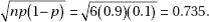
(e) Since nq = 40(1 – 0.90) = 4, the normal approximation to the binomial is not recommended. However, a direct binomial calculation yields
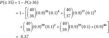
[Or simply use binomcdf(40, .9, 35) on the TI-84.] With such a high probability, there is no evidence to conclude that Jordan’s average has dropped!
2. (a) With 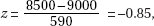 Table A gives a probability of 0.1977 ≈ 0.2.
(b) For example, letting 0 and 1 represent caplets containing less than 8500 units and 2 through 9 represent caplets containing more than 8500 units, we can read off digits until we find two containing less than 8500 caplets. Five simulations would yield
841770 67571761 31558251 50681 435410
giving 6, 8, 8, 5, and 6 tablets sampled before finding two with less than 8500 units apiece.
(c) The probability of a caplet having more than 9000 units is 0.5, and thus one would expect to find two caplets with more than 9000 units much quicker than finding two caplets with less than 8500 units. Thus the first histogram results from looking for two caplets with more than 9000 units and the second histogram results from looking for two caplets with less than 8500 units.
(d) An estimate for the expected value is obtained by
 xP (x) = 2(0.03) + 3(0.05) + 4(0.09) + 5(0.10) + … + 24(0.01) = 9.44
12 Sampling Distributions
Answers Explained
MULTIPLE-CHOICE
1. (C) The larger the sample, the smaller the spread in the sampling distribution. Bias has to do with the center, not the spread, of a sampling distribution. Sample statistics are used to make inferences about population proportions. Statistics from smaller samples have more variability.
2. (E) It is always true that the sampling distribution of x has mean µ and standard
deviation  . In addition, the sampling distribution will be normal if the population
is normal and will be approximately normal if n is large even if the population is not
normal. and σ are not equal unless n = 1.
3. (A) The sampling distribution of  has a standard deviation
  which is smaller with larger n. While the sampling distribution of is never exactly normal, it is considered close to normal provided that both np and n(1 – p) are large enough (greater than 10 is a standard guide).
4. (B) Sample proportions are an unbiased estimator for the population proportion, and larger sample sizes lead to reduced variability.
5. (E) The sampling distribution of x has mean µ, standard deviation  and shape, which becomes closer to normal with larger n.
6. (A) The maximum of a sample is never larger than the maximum of the population, so the mean of the sample maximums will not be equal to the population maximum. (A sampling distribution is unbiased if its mean is equal to the population parameter.)
7. (E) All are unbiased estimators for the corresponding population parameters; that is, the means of their sampling distributions are equal to the population parameters.
8. (D) The sample is given to be random, both np = (400)(0.34) = 136 10 and n(1 – p) = (400)(0.66) = 264 10, and our sample is clearly less than 10% of all people. So the sampling distribution of is approximately normal with mean 0.34 and standard deviation  and
and 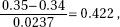 the probability that the sample proportion is between 0.30 and 0.35 is normalcdf(–1.688, .422)= 0.618. [Or normalcdf(.3, .35, .34, .0237)= 0.618.]
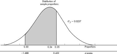
9. (B) The sample is given to be random, both np = (300)(0.12) = 36 10 and n(1 – p) = (300)(0.88) = 264 10, and our sample is clearly less than 10% of all butterfly larvae. So the sampling distribution of is approximately normal with mean µ = 0.12 and standard deviation 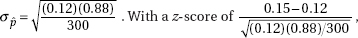 the probability that the sample proportion is more than 15% is
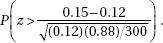
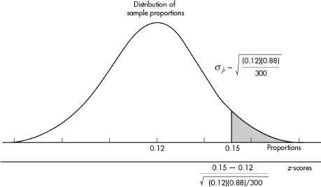
10. (C) We have a random sample that is less than 10% of the high school football population. With a sample size of 48, the central limit theorem applies, and the sampling distribution of x is approximately normal with mean µx = 355 and standard deviation 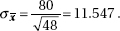 The z-scores of 340 and 360 are
 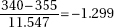 and
and 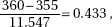 the probability of a sample mean between 340 and 360 is normalcdf(-1.299,.433)= 0.571. [Or normalcdf(340,360,355,11.547)= 0.571.]
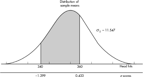
11. (A) We have a random sample that is less than 10% of all schools. With a sample size of 30, the central limit theorem applies, and the sampling distribution of x is approximately normal with mean µx = 1200 and standard deviation  The z-score of 1000 is
  and the probability of a sample mean over 1000 is
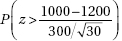
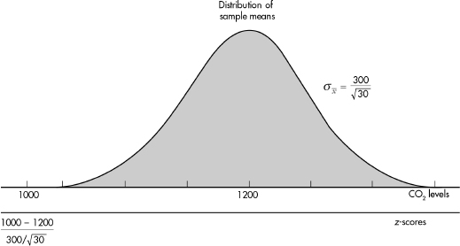
12. (B) We have two independent random samples, each less than 10% of their respective populations, and we note that n1p1 = 75(0.43) = 32.25, n1(1 – p1) = 75(0.57) = 42.75, n2p2 = 80(0.37) = 29.6, and n2(1 – p2) = 80(0.63) = 50.4 are all 10. Thus the sampling distribution of  1 – 2 is roughly normal with mean
 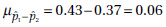 and standard deviation
 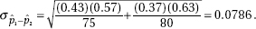 The z-score of 0.05 is
 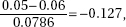 the z-score of 0.10 is
 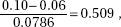 and normalcdf(-.127,.509)= 0.245. [Or normalcdf(.05,.10,.06,.0786)= 0.245.]
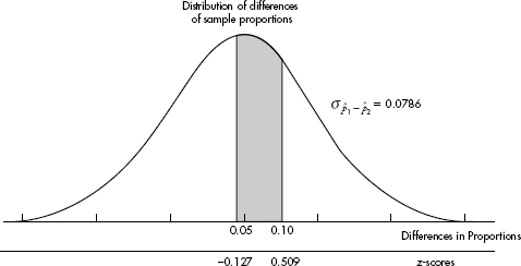
13. (A) We have independent random samples, each less than 10% of babies, and both sample sizes are 40 30, so the sampling distribution of  1 – 2 is roughly normal with mean
 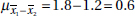 and standard deviation
 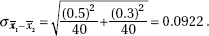 The z-score of 0.75 is
 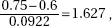 and normalcdf(1.627,1000)= 0.0519. [Or normalcdf(.75,1000,.6,.0922)= 0.0519.]
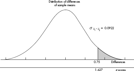
14. (B) The t-distributions are symmetric and mound-shaped, and they have more, not less, spread than the normal distribution.
15. (A) The larger the number of degrees of freedom, the closer the curve to the normal curve. While around the 30 level is often considered a reasonable approximation to the normal curve, it is not the normal curve.
FREE-RESPONSE
1. (a) 0.58
(b) This is a binomial with n = 3 and p = 0.58.

or 1–binomcdf(5,.58,2)= 0.647.
(c) The sample is given to be random, both np = (350)(0.58) = 203 10 and n(1 – p) = (350)(0.42) = 147 10, and our sample is clearly less than 10% of all Americans. So the sampling distribution of is approximately normal with mean 0.58 and standard deviation 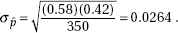 With a z-score of
 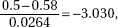 the probability that the sample proportion is greater than 0.5 is normalcdf(−3.030,1000)= 0.9988.
[Or normalcdf (.5,1,.58,.0264)= 0.9988.]
2. (a) We do not know the shape of the distribution of the amount individual teenage drivers pay for insurance, so there is no way of calculating the probability a randomly chosen teenage driver pays over $2400 a year for auto insurance.
(b) 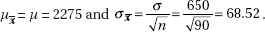
(c) With this large a sample size (90 40), the central limit theorem tells us that the sampling distribution of x is approximately normal. We calculate

3. (a) The z-scores corresponding to cumulative probabilities of 0.25 and 0.75 are ±0.6745. Thus Q1 = 374 – (0.6745)(38.55) = 348.00, Q3 = 374 + (0.6745)(38.55) = 400.00, and IQR = Q3 – Q1 = 400 – 348 = 52 hours.
(b) From part (a), we have that the probability of less than 400 deprived hours is 0.75, and thus the probability of being more than 400 deprived hours is 0.25. Now we have a binomial with n = 3 and p = 0.25. P(majority > 400) = P(2 or 3 are > 400) = 3(0.25)2(0.75) + (0.25)3 = 0.15625.
(c) The sampling distribution of the sample means is approximately normal (because the original population is normal) with mean µx = µ = 374 and standard deviation 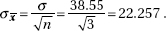 The z-score of 400 is
  and the probability of a sample mean over 400 is normalcdf(1.168,1000)= 0.121. [Or normalcdf(400,1000,374,22.257)= 0.121.]
4. (a) 
[Or normalcdf(4250,10000,4000,125)= 0.0228.]
(b) The original population is normal so the sampling distribution of is normal with mean µ = µ = 4000 and standard deviation 
(c) 
[Or normalcdf(0,3950,4000,19.764)= 0.0057.]
(d) The answer to part (a) would be affected because it assumes a normal population. The other answers would not be affected because for large enough n, the central limit theorem gives that the sampling distribution of is roughly normal regardless of the distribution of the original population.
INVESTIGATIVE TASK
(a) Using a calculator, find μ = 12 and σ = 5.0596.
(b)

(c) 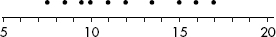
(d) µx = 12 and x = 3.0984.
(e) 
(f) If N is very large,  is approximately equal to 1, and so the expression is approximately equal to
13 Confidence Intervals
Answers Explained
MULTIPLE-CHOICE
1. (C) The critical z-scores will go from ±1.96 to ±2.576, resulting in an increase in the interval size:  or an increase of 31%.
2. (D) Increasing the sample size by a multiple of d divides the interval estimate by  .
.
3. (A) The margin of error varies directly with the critical z-value and directly with the standard deviation of the sample, but inversely with the square root of the sample size. The value of the sample mean and the population size do not affect the margin of error.
4. (D) Although the sample proportion is between 77% and 87% (more specifically, it is 82%), this is not the meaning of ±5%. Although the percentage of the entire population is likely to be between 77% and 87%, this is not known for certain.
5. (E) The 95% refers to the method: 95% of all intervals obtained by this method will capture the true population parameter. Nothing is certain about any particular set of 20 intervals. For any particular interval, the probability that it captures the true parameter is 1 or 0 depending upon whether the parameter is or isn’t in it.
6. (E) There is no guarantee that 13.4 is anywhere near the interval, so none of the statements are true.
7. (E) The critical z-score with 0.005 in each tail is 2.576 (from last line on Table B or invNorm(0.005) on the TI-84), and 
8. (A) The margin of error has to do with measuring chance variation but has nothing to do with faulty survey design. As long as n is large, s is a reasonable estimate of ; however, again this is not measured by the margin of error. (With t-scores, there is a correction for using s as an estimate of .)
9. (B) The critical z-score with 0.01 in the tails is 2.326 (invNorm(0.01) on the TI-84), and 
10. (B) 1-PropZInt on the TI-84 gives (0.72316, 0.77684).
11. (D) 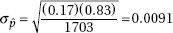 z(0.0091) = 0.02 z = 2.20, 0.9861 – 0.0139 = 97.2%
12. (C) 
13. (E) 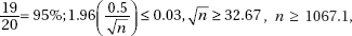 and so the pollsters should have obtained a sample size of at least 1068. (They actually interviewed 1148 people.)
14. (E) LOL, OMG, the critical t-score with 0.02 in the tails is 2.088 (Table B or invt(0.02,79) on the TI-84), and 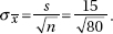
15. (C) TInterval on the TI-84 gives (28.052, 28.948).
16. (D) 
17. (E) Using t-scores:

18. (E) 
19. (E) To divide the interval estimate by d without affecting the confidence level, multiply the sample size by a multiple of d2. In this case, 4(50) = 200.
20. (A) 2-PropZInt on the TI-84 gives (0.07119, 0.30155) or 0.18637 ± 0.11518.
21. (B)
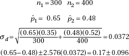
22. (D) 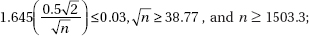 the researcher should choose a sample size of at least 1504.
23. (A) 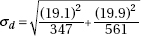 and with df = min(347 – 1, 561 – 1), critical t-scores are ±1.97.
24. (B) 2-SampTInt on the TI-84 gives (3.1333, 5.6667) or 4.4 ± 1.2667.
25. (C) 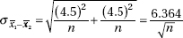
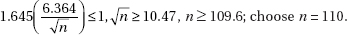
26. (A) The sample mean is at the center of the confidence interval; the lower confidence level corresponds to the narrower interval.
27. (C) Narrower intervals result from smaller standard deviations and from larger sample sizes.
28. (E) Only III is true. The 90% refers to the method; 90% of all intervals obtained by this method will capture µ. Nothing is sure about any particular set of 100 intervals. For any particular interval, the probability that it captures µ is either 1 or 0 depending on whether µ is or isn’t in it.
29. (E) In determining confidence intervals, one uses sample statistics to estimate population parameters. If the data are actually the whole population, making an estimate has no meaning.
30. (B) 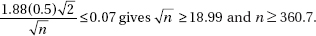
31. (E) With df = 15 – 1 = 14 and 0.05 in each tail, the critical t-value is 1.761.
32. (D) x = 4.048, s = 2.765, df = 20, and
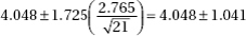
33. (C) TInterval on the set of differences gives (7.8514, 15.371) or 11.6112 ± 3.7598.
34. (C) TInterval on the TI-84 gives (2.9389, 3.4611) or 3.2 ± 0.2611.
35. (E) The critical t-values with df = 25 – 2 = 23 are ±2.500. Thus, we have b1 ± t∗ × SE(b1) = 0.008051 ± (2.500)(0.001058).
36. (E) The critical t-values with df = n – 2 = 8 are ±2.306. Thus, we have b ± t∗ × SE(b) = –2.16661 ± 2.306(1.03092) = –2.16661 ± 2.3773 or (–4.54,0.21).
37. (E) While there is clearly a positive association between smoking levels and hazard ratios, this was an observational study, not an experiment, so cause and effect (as implied in I, II, and III) is not an appropriate conclusion. The margins of error of the confidence intervals become greater (less precision) with heavier smoking.
FREE-RESPONSE
1. (a) First, identify the confidence interval and check the conditions: This is a one-sample z-interval for the proportion of all voters who believe competence is more important than character. It is given that this is a random sample, we calculate n = 1000(0.57) = 570 10 and n = 1000(0.43) = 430 10, and n = 1000 is less than 10% of all voters.
Second, calculate the interval:
Calculator software (such as 1-PropZInt on the TI-84) gives (0.53932, 0.60068). [For instructional purposes in this review book, we note that = 0.57 and 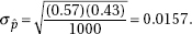 The critical z-scores associated with the 95% level are ±1.96. Thus the confidence interval is 0.57 ± 1.96(0.0157) = 0.57 ± 0.031, or between 53.9% and 60.1%.]
Third, interpret in context:
We are 95% confident that between 53.9% and 60.1% of all voters believe competence is more important than character.
(b) Explain to your parents that by using a measurement from a sample we are never able to say exactly what a population proportion is; rather we are only able to say we are confident that it is within some range of values, in this case between 53.9% and 60.1%.
(c) In 95% of all possible samples of 1000 voters, the method used gives an estimate that is within three percentage points of the true answer.
2. (a) First, identify the confidence interval and check the conditions:
This is a one-sample z-interval for the proportion of family members who come down with H1N1 after an initial family member does in this state, that is, 
It is given that this is a random sample, and we calculate n = 129 10 and n(1 – ) = 747 10.
Second, calculate the interval:
Calculator software (such as 1-PropZInt on the TI-84) gives (0.12757, 0.16695).
[For instructional purposes in this review book, we note that  and 0.147 ± 1.645
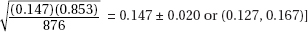
Third, interpret in context:
We are 90% confident that the proportion of family members who come down with H1N1 after an initial family member does in this state is between 0.127 and 0.167.
(b) Because 1/8 = 0.125 is not in the interval of plausible values for the population proportion, there is evidence that the proportion of family members who come down with H1N1 after an initial family member does in this state is different from the 1 in 8 chance concluded in the published study.
(c) 0.147 ± 2.576  = 0.147 ± 0.031 or (0.116, 0.178) which does include 0.125, so in this case there is not evidence that the proportion of family members who come down with H1N1 after an initial family member does in this state is different from the 1 in 8 chance concluded in the published study.
3. (a) First, identify the confidence interval and check the conditions:
This is a two-sample z-interval for pUS – pUK, the difference in population proportions of new births to unmarried women in the United States and United Kingdom, that is,
It is given that these are random samples, they are clearly independent, and we calculate nUS US = (500)(0.412) = 206 10,
nUS (1 – US) = (500)(0.588) = 294 10,
nUK UK = (400)(0.465) = 186 10, and
nUK (1 – UK) = (400)(0.535) = 214 10.
Second, calculate the interval:
Calculator software (such as 2-PropZInt on the TI-84) gives (–0.1182, 0.01219). [For instructional purposes in this review book, we note that:

Third, interpret in context:
We are 95% confident that the difference in proportions, pUS – pUK, of new births to unmarried women in the United States and United Kingdom is between –0.118 and 0.012.
(b) Because 0 is in the interval of plausible values for the difference of population proportions, this confidence interval does not support the belief by the UN health care statistician that the proportions of new births to unmarried women is different in the United States and United Kingdom.
4. (a) We are calculating one-sample t-intervals for the mean price of gas in inner city stations and for the mean price of gas in suburban stations. In each case, we are given random samples and the sample sizes of 40 and 120 are large enough so that by the CLT the distributions of sample means are approximately normal and t-intervals may be found. We assume that the sample sizes are less than 10% of the populations of all gas stations. Calculator software (such as TInterval on the TI-84) gives (3.434, 3.466) for inner city stations and (3.3655, 3.3945) for suburban stations. That is, we are 95% confident that the mean price for gas in inner city stations is between $3.434 and $3.466, and are 95% confident that the mean price for gas in suburban stations is between $3.3655 and $3.3945.
(b) Because the sample size of inner city stations is smaller.
(c) Yes, because the standard deviation of the set of sample means is  0.0079, and so $3.50 is more than three standard deviations away from $3.45. Thus the probability that the true mean is this far from the sample mean is extremely small.
5. (a) We are calculating a one-sample t-interval for the mean number of riders per car during rush hour. We are given a random sample, the sample size of 30 is assumed to be less than 10% of all subway cars, and assuming that the sample data are unimodal and reasonably symmetric with no extreme values, the sample size of 30 is large enough so that by the CLT the distribution of sample means is approximately normal and a t-interval may be found. Calculator software (such as TInterval on the TI-84) gives (81.67, 85.33). [For instructional purposes in this review book, we note that: With df = n – 1 = 29, the critical t-scores from Table B (or from InvT on the TI-84) are ±1.699, and  We are 90% confident that the mean number of riders per car during rush hour is between 81.67 and 85.33.
(b)  so you must choose a random sample of at least 95 subway cars.
6. (a) Calculator software (such as TInterval on the TI-84) gives (–29,337, 421,337), or we are 95% confident that the mean salary of all basketball salaries from the population from which this sample was taken is between –$29,337 and $421,337. [For instructional purposes in this review book, we note that with df = 9,

(b) We must assume the sample is an SRS and that basketball salaries are normally distributed. This does not seem reasonable—the salaries are probably strongly skewed to the right by a few high ones. With the given mean and standard deviation, and noting that salaries are not negative, clearly we do not have a normal distribution, and furthermore, the sample size, n = 10, is too small to invoke the CLT. The calculated confidence interval is not meaningful.
7. This is a one-sample t-interval for the mean number of calories of all breakfast cereals. We are given that we have a random sample, and the nearly normal condition seems reasonable from, for example, either a stemplot or a normal probability plot:
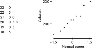
Under these conditions the mean calories can be modeled by a t-distribution with n – 1 = 10 – 1 = 9 degrees of freedom.
Calculator software (such as TInterval using Data on the TI-84) gives (195.32, 215.68). [For instructional purposes in this review book, we note that a one-sample t-interval for the mean gives:
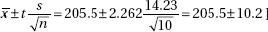
We are 95% confident that the true mean number of calories of all breakfast cereals is between 195.3 and 215.7.
8. (a) First, identify the confidence interval and check the conditions:
This is a two-sample t-interval for µNRW – µRW, the difference in population means of BPA body concentrations in non-retail workers and retail workers, that is,
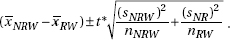
It is given that these are random samples, it is reasonable to assume the samples are independent, and both samples sizes (528 and 197) are large enough so that by the CLT, the distributions of sample means are approximately normal and a t-interval may be found.
Second, calculate the interval:
Calculator software (such as 2-SampTInt on the TI-84) gives (–0.9521, –0.7479) with df = 332.3.
Third, interpret in context:
We are 99% confident that the difference in means of BPA body concentrations in non-retail and retail workers (non-retail mean minus retail mean) is between –0.75 and –0.95 µg/L.
(b) Because 0 is not in the interval of plausible values for the difference of population means, and the entire interval is negative, the interval does support the belief that retail workers carry higher amounts of BPA in their bodies than non-retail workers.
9. We first check conditions: we must assume use of randomization. The scatterplot is roughly linear, and there is no apparent pattern in the residuals plot.
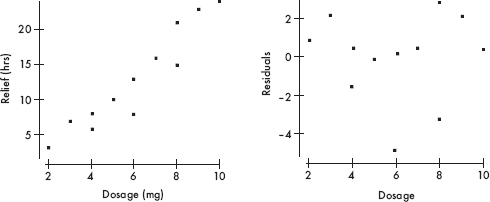
The distribution of the residuals is very roughly normal.
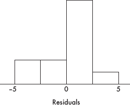
(a) Now using the statistics software on a calculator gives

(b) Using calculator software (such as LinRegTInt on the TI-84 with the data in Lists) gives (2.1631, 3.1898). We are 90% confident that each additional gram of the new drug is associated with an average of between 2.16 and 3.19 more hours of allergy relief.
10. (a) Assuming that all assumptions for regression are met, the y-intercept and slope of the equation are found in the Coeff column of the computer printout.

where both the selling price and the assessed value are in $1000.
(b) From the printout, the standard error of the slope is sb1= 0.08192. With df = 18 and 0.005 in each tail, the critical t-values are ±2.878. The 99% confidence interval of the true slope is:

We are 99% confident that for every $1 increase in assessed value, the average increase in selling price is between $0.79 and $1.27 (or for every $1000 increase in assessed value, the average increase in selling price is between $790 and $1270).
11. (a)  So the margin of error is ±2.65%.
(b) We are 95% confident that between 71.35% and 76.65% of smokers would like to give up smoking.
(c) If this survey were conducted many times, we would expect about 95% of the resulting confidence intervals to contain the true proportion of smokers who would like to give up smoking.
(d) Smoking is becoming more undesirable in society as a whole, so some smokers may untruthfully say they would like to stop.
(e) To be more confident we must accept a wider interval.
(f) All other things being equal, the greater the sample size, the smaller the margin of error.
AN INVESTIGATIVE TASK
(a) 
(b) 33.9% of the variability in career earnings is associated with years as a pro. However, looking at the scatterplot, if Serena’s data point, (18, 54.38), is removed, there appears to be no linear relationship at all. (Serena’s data point is called an influential point.)
(c) 2.69 + 1.6752(15) = $27.82 million, and 2.69 + 1.6752(30) = $52.95 million. The estimate for 15 years might be reasonable, but the one for 30 years is not; it is an extrapolation far from the given sample data points.
(d) We note that the scatterplot looks very roughly linear, there is no major pattern in the residual plot, and the histogram of residuals is very roughly unimodal and symmetric. With df = n – 2 = 8 and 90% confidence, Table B, the t-distribution table, gives critical t-scores of ±1.860. Then 1.6752 ± 1.860(0.8264) = 1.6752 ± 1.537. We are 90% confident that the true slope of the regression line linking career earnings to years as a pro is between $0.138 million and $3.212 million. The interpretation in context: We are 90% confident that for each additional year as a tennis professional, the career earnings go up by between $0.138 million and $3.212 million, on average.
(e) 2.69 ± 1.860(10.78) = 2.69 ± 20.05. We are 90% confident that the true y-intercept of the regression line linking career earnings to years as a pro is between –$17.36 million and $22.74 million. The interpretation in context: This y-intercept has no meaning in context because it references career earnings when there are 0 years as a pro.
(f) The model with 0 intercept makes more sense in this situation. When there are 0 years as a pro, the career earnings should be 0.
14 Tests of Significance—Proportions and Means
Answers Explained
MULTIPLE-CHOICE
1. (E) We attempt to show that the null hypothesis is unacceptable by showing that it is improbable; however, we cannot show that it is definitely true or false. Both the null and alternative hypotheses are stated in terms of a population parameter, not a sample statistic. These hypotheses tests assume simple random samples.
2. (E) The P-value of a test is the probability of obtaining a result as extreme (or more extreme) as the one obtained assuming the null hypothesis is true. Small P-values are evidence against the null hypothesis. The null and alternative hypotheses are decided upon before the data come in.
3. (E) The parameter of interest is µ = the mean number of hours per week which middle school students spend in video arcades.
4. (C) The alternative hypothesis is always an inequality, either <, or >, or ≠. In this case, the concern is whether middle school students are spending an average of more than two hours per week in video arcades.
5. (E) The P-value is a conditional probability; in this case, there is a 0.032 probability of an observed difference in sample proportions as extreme (or more extreme) as the one obtained if the null hypothesis is assumed to be true.
6. (C) This is a hypothesis test with H0: breaking strength is within specifications, and Ha: breaking strength is below specifications. A Type I error is committed when a true null hypothesis is mistakenly rejected.
7. (C) A Type II error is a mistaken failure to reject a false null hypothesis or, in this case, a failure to realize that a person really does have ESP.
8. (B) 
[On the TI-84, normalcdf(–1000,–1.242) = 0.107.]
9. (C) Medications having an effect shorter or longer than claimed should be of concern, so this is a two-sided test: Ha: µ ≠ 58.4, and df = n – 1 = 40 – 1 = 39.
10. (B) The level of significance is defined to be the probability of committing a Type I error, that is, of mistakenly rejecting a true null hypothesis.
11. (D) 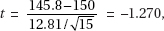 and with df = 14, P = 0.112. With this high P-value (0.112 > 0.10), the students do not have sufficient evidence to reject the fast food chain’s claim. (On the TI-84, T-Test gives P = 0.112423.)
12. (A) With unknown population standard deviations, the t-distribution must be used, 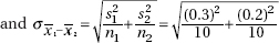
13. (B) A Type I error means that the null hypothesis is true (the weather remains dry), but you reject it (thus you needlessly cancel school). A Type II error means that the null hypothesis is wrong (the snow storm hits), but you fail to reject it (so school is not canceled).
14. (E) With  With a P-value this high (0.141 > 0.10), the government does not have sufficient evidence to reject the company’s claim. (On the TI-84, 1PropZTest gives P = 0.140956.)
15. (D)  This is a two-sided test (H0: p1 – p2 = 0, Ha: p1 – p2 ≠ 0) with
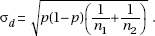
16. (E) There is a different answer for each possible correct value for the population parameter.
17. (A) This is a one-sided z-test, 
18. (B) P(at least one Type I error) = 1 – P(no Type I errors) = 1 – (0.99)5 = 0.049
19. (C) A larger sample size n reduces the standard deviation of the sampling distributions resulting in narrower sampling distributions so that for the given sample statistic, the P-value is smaller, and the probabilities of mistakenly rejecting a true null hypothesis or mistakenly failing to reject a false null hypothesis are both decreased. Furthermore, a lower Type II error results in higher power.
20. (E) The two-sample hypothesis test is not the proper one and can only be used when the two sets are independent. In this case, there is a clear relationship between the data, in pairs, one pair for each student, and this relationship is completely lost in the procedure for the two-sample test. The proper procedure is to run a one-sample test on the single variable consisting of the differences from the paired data.
21. (C) With a smaller  , that is, with a tougher standard to reject H0, there is a greater chance of failing to reject a false null hypothesis, that is, there is a greater chance of committing a Type II error. Power is the probability that a Type II error is not committed, so a higher Type II error results in lower power.
22. (B) If the null hypothesis is far off from the true parameter value, there is a greater chance of rejecting the false null hypothesis and thus a smaller risk of a Type II error. Power is the probability that a Type II error is not committed, so a lower Type II error results in higher power.
23. (C) With  = 6.48 and s = 1.388,
 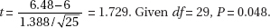 [On the TI-84, T-Test gives P = 0.048322.]
24. (C) If the alternative is true, the probability of failing to reject H0 and thus committing a Type II error is 1 minus the power, that is, 1 – 0.75 = 0.25.
25. (B) 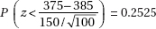
[On the TI-84, normalcdf(–100, –10/15) = 0.252492.]
FREE-RESPONSE
1. The parameter of interest is µ = the mean tire pressure in the front right tires of cars with recommended tire pressure of 35 psi. H0: µ = 35 and Ha: µ ≠ 35.
2. (a) The P-value of 0.138 gives the probability of observing a sample proportion of GBS complications as great or greater as the proportion found in the study if in fact the proportion of GBS complications is 0.000001.
(b) Since 0.138 > 0.10, there is no evidence to reject H0, that is, there is no evidence that under the new vaccine the proportion of GBS complications is greater than 0.000001 (one in a million).
(c) The null hypothesis is not rejected, so there is the possibility of a Type II error, that is of mistakenly failing to reject a false null hypothesis. A possible consequence is continued use of vaccine with a higher rate of serious complications than is acceptable.
3. (a) The P-value of 0.0197 gives the probability of observing a sample mean of 1002.4 or greater if in fact this system results in a mean E. coli concentration of 1000 MPN/100 ml.
(b) Since 0.0197 < 0.05, there is evidence to reject H0, that is, there is evidence that the mean E. coli concentration is greater than 1000 MPN/100 ml, and the system is not working properly.
(c) With rejection of the null hypothesis, there is the possibility of a Type I error, that is of mistakenly rejecting a true null hypothesis. Possible consequences are that sales of the system drop even though the system is doing what it claims, or that the company performs an overhaul to fix the system even though the system is operating properly.
4. (a) This was an observational study as no treatments were imposed. It would have been highly unethical to impose treatments, that is, to instruct randomly chosen volunteers to smoke, drink, skip exercise, and eat poorly.
(b) H0: p4 = p0, Ha: p4 > p0 where p4 is the proportion of adults with all four bad habits who die during a 20-year period, and p0 is the proportion of adults with none of the four bad habits who die during a 20-year period. (Note that the hypotheses are about the population of all adults with and with none of the four bad habits, not about the volunteers who took part in the study.)
(c) A Type I error, that is, a mistaken rejection of a true null hypothesis, would result in people being encouraged to not smoke, not drink, exercise, and eat well, when these actions actually will not help decrease 20-year death rates.
(d) A Type II error, that is, a mistaken failure to reject a false null hypothesis, would result in people thinking that smoking, drinking, inactivity, and poor diet don’t increase 20-year death rates, when actually they do contribute to higher 20-year death rates.
(e) Calculator software (such as 2-PropZTest on the TI-84) gives P = 0.000.
[For instructional purposes in this review book, we note that:
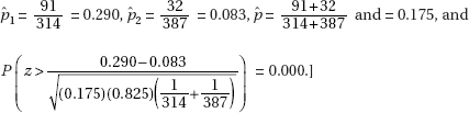
If the null hypothesis were true, that is, if there was no difference in the 20-year death rates between people with all four bad habits and people with none of the bad habits, then the probability of sample proportions with a difference as extreme or more extreme than observed is 0.000 (to three decimals).
5. First, state the hypotheses:
H0: p = 0.174 and Ha: p > 0.174. (If asked to state the parameter, then state
“where p is the proportion of AAUP members who own Roth IRAs.”)
Second, identify the test by name or formula and check the assumptions.
This is a one-sample z-test for a population proportion.
Assumptions: Random sample (given), np = 750(0.174) = 130.5 10, n(1 – p) = 750(0.826) = 619.5 10, and the sample size, n = 750, is less than 10% of all AAUP members.
Third, calculate the test statistic z and the P-value. Calculator software (such as 1-PropZTest on the TI-84) gives z = 1.878 and P = 0.030.
[For instructional purposes in this review book, we note that

Fourth, linking to the P-value, give a conclusion in context.
With a P-value this small, 0.030 < 0.05, there is sufficient evidence to reject H0, that is, there is evidence that more than 17.4% of AAUP members own Roth IRAs.
6. First, state the hypotheses: H0: µ = 593 and Ha: µ ≠ 593 (If asked to state the parameter, then state “where µ is the mean discharge rate (in 1000 ft3/sec) at the mouth of the Mississippi River.”)
Second, identify the test by name or formula and check the assumptions:
This is a one-sample t-test for the mean with  Assumptions: The measurements were taken at random times, the sample size, n = 10, is less than 10% of all possible measurements, and either a dotplot of the sample is roughly unimodal and symmetric or the normal probability plot is roughly linear:
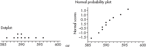
Third, calculate the test statistic t and the P-value:
Calculator software (such as T-Test using Data on the TI-84) gives t = –2.7116 and P = 0.0239. [For instructional purposes in this review book, we note that x = 590.5 and s = 2.9155 which gives
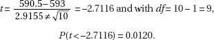
Since this is a two-sided test, we double this value to find the P-value to be P = 0.0240.]
Fourth, linking to the P-value, give a conclusion in context: With a P-value this small, 0.0239 < 0.05, there is sufficient evidence to reject H0, that is, there is evidence that the long accepted measure of the discharge rate at the mouth of the Mississippi River has changed.
7. First, state the hypotheses: H0: pB – pG = 0 (or pB = pG) and Ha: pB – pG > 0 (or pB > pG). If asked to state the parameters, then state “where pB is the proportion of high school boys who meet the recommended level of physical activity, and pG is the proportion of high school girls who meet the recommended level of physical activity.”)
Second, identify the test by name or formula and check the assumptions:
This is a two-sample z-test for proportions. Assumptions: Independent random samples (given), and nB B = 370 10, nB (1 – B) = 480 10, nGG = 218 10, and nG (1 – G) = 362 10.
Third, calculate the test statistic z and the P-value. Calculator software (such as 2-PropZTest on the TI-84) gives z = 2.2427 and P = 0.012. (For instructional purposes in this review book, we note that
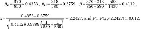
Fourth, linking to the P-value, give a conclusion in context. With a P-value this small (0.012 < 0.05), there is evidence that the proportion of high school boys who meet the recommended level of physical activity is greater than the proportion of high school girls who meet the recommended level of physical activity.
8. First, state the hypotheses: H0: µNFL – µ10 = 0 (or µNFL = µ10) and Ha: µNFL – µ10 < 0 (or µNFL < µ10) (or “>” depending on choice of variables). (If asked to state the parameters, then state “where µNFL is the mean attendance at NFL games and µ10 is the mean attendance at Big 10 football games.”]
Second, identify the test by name or formula and check the assumptions: This is a two-sample t-test for means. Assumptions: Independent random samples (given), both samples sizes, 35 and 30, are large enough so that by the CLT, the distribution of sample means is approximately normal and a t-test may be run, and the sample sizes, nNFL = 35 and n10 = 30, are less than 10% of all NFL and Big 10 football games.
Third, calculate the test statistic t and the P-value. Calculator software (such as 2-SampTTest on the TI-84) gives t = –0.8301, df = 49.3, and P = 0.2052. [For instructional purposes in this review book, we note that:
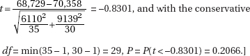
Fourth, linking to the P-value, give a conclusion in context. With a P-value this large, 0.2052 > 0.05, there is not sufficient evidence to reject H0, that is, there is not sufficient evidence that the average attendance at Big 10 Conference football games is greater than that at NFL games.
9. (a) One block consists of the 500 patients who have had a mini stroke in the previous year, and a second block consists of the 500 patients who have not. In one block, number the patients 1 through 500, and then using a random number generator, pick numbers between 1 and 500, throwing out repeats, until 250 patients are picked. Assign surgery to these patients and stents to the remaining 250. Repeat for the other block.
(b) One method is to increase the sample size, resulting in a reduction in the standard error of the sampling distribution, which in turn increases the probability of rejecting the null hypothesis if it is false. A second method is to increase , the significance level, which in turn also increases the probability of rejecting the null hypothesis if it is false. In either case, there is increased probability of detecting any difference in the proportions of patients suffering major complications between the surgery and stent recipients.
10. The data come in pairs, and the two-sample test does not apply the knowledge of what happened to each individual driver (the condition of independence of the two samples is violated). The appropriate test is a one-population, small-sample hypothesis test on the set of differences: {0, –5, 3, –4, –3, 1, –2, –2, –1, –1}. We proceed as follows:
First, state the hypotheses: H0: µD = 0, Ha: µD ≠ 0 (If asked to state the parameter, then state “where µD is the mean difference in reaction times between DWI and DWT.”)
Second, identify the test and check the assumptions: This is a paired t-test, that is, a single-sample hypothesis test on the set of differences.
The data are paired because they are measurements on the same individuals under DWI and DWT.
The reaction times of any individual are assumed independent of the reaction times of the others, so the differences are independent.
We must assume that the volunteers are a representative sample.
Either a dotplot of the sample is roughly unimodal and symmetric or the normal probability plot is roughly linear:
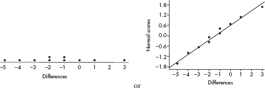
The sample size, n = 10, is less than 10% of all possible drivers.
Third, calculate the test statistic t and the P-value: Calculator software (such as T-Test and Data on the TI-84) gives t = –1.871 and P = 0.094174. [For instructional purposes in this review book, we note that x = –1.4 and s = 2.366 giving 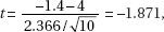 and with df = 10 – 1 = 9, P(t < –1.871) = 0.0471. Since this is a two-sided test, we double this value to find the P-value to be P = 0.0942.]
Fourth, linking to the P-value, give a conclusion in context: With a P-value this small, 0.0942 < 0.10, there is sufficient evidence to reject H0, that is, there is evidence at the 10% significance level of a difference between the mean effect on reaction time between DWI and DWT. Or, with a P-value this large, 0.0942 > 0.05, there is not sufficient evidence to reject H0, that is, there is not sufficient evidence at the 5% significance level of a difference between the mean effect on reaction time between DWI and DWT.
INVESTIGATIVE TASKS
1. (a) 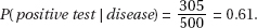
(b) 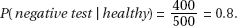
(c) 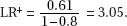 A positive test given a diseased subject and a negative test given a healthy subject are both desired outcomes, so higher values for both Sensitivity and Specificity are good. Higher values of Sensitivity, the numerator of LR+, lead to greater values of LR+. Higher values of Specificity give lower values of 1 – Specificity, the denominator of LR+, again leading to greater values of LR+.
(d) The estimated P-value is the proportion of the simulated statistics that are less than or equal to the sample statistic of 4.7. Counting values in the dotplot gives a P-value of 0.04. With a P-value this small, there is evidence that the population LR+ is below the desired value of 5.0.
2. (a) Different schemes are possible. For example, assign each material a single-digit number, such as A-0, B-1, C-2, D-3, E-4, F-5, G-6, H-7, I-8, J-9. Then read off the digits from the random number list, one at a time, throwing away any repeats, until each of the materials have been picked (or nine have been picked, as the last one left will go last). The order of picking then gives the order of being tested. Using this scheme we would get the following order:

(b) The mean drilling times in the ten materials are 4.69 seconds for Drill 1 and 4.77 seconds for Drill 2.
The proper hypothesis test is a matched pairs t-test on the set of differences, {0, –0.3, 0.1, –0.2, –0.1, –0.4, 0, 0.3, –0.1, –0.1}
First, state the hypotheses: H0: µd = 0, Ha: µd ≠ 0. (If asked to state the parameter, then state “where µd is the difference in mean drilling times of the two drills through different materials.”)
Second, identify the test by name or formula and check the assumptions: This is a one-sample t-test for the mean of paired differences.
Assumptions: random samples (given), n = 10 is less than 10% of all possible materials, hardnesses, and thicknesses, and either a dotplot of the difference sample is roughly unimodal and symmetric, or the normal probability plot is roughly linear:
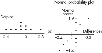
Third, calculate the test statistic t and the P-value: Calculator software (such as T-Test with Data on the TI-84) gives t = –1.272 and P = 0.2353. [For instructional purposes in this review book, we note that:
x = –0.08 and s = 0.1989 which gives  and with df = 10 – 1 = 9, P(t < –1.272) = 0.1176. Since this is a two-sided test, we double this value to find the P-value to be P = 0.2352.]
Fourth, linking to the P-value, give a conclusion in context. With a P-value this large, 0.2353 > 0.05, there is not sufficient evidence to reject H0, that is, there is not sufficient evidence of a difference in mean drilling times of the two drills through different materials.
3. (a) The conditions for a one-sample z-test on a population proportion include that both n 10 and n(1 – ) 10. In this case, n = 12 but n(1 – ) = 2.
(b) First, state the hypotheses: H0:p = 0.5 and Ha: p > 0.5, [If asked to state the parameter, then state “where p is the proportion of soccer matches for which Paul the octopus can correctly predict the winning team.”]
Second, identify the test and check the assumptions:
This is a test of a binomial model.
For each trial there are two outcomes (Paul has a choice of two boxes of mussels), the trials are independent, and the probability of Paul picking a winner can be assumed to be the same for each trial. We are given that the 14 matches are a random sample of all matches.
Third, calculate the P-value: With p = 0.5,

Fourth, linking to the P-value, give a conclusion in context: With a P-value this small, 0.00647 < 0.05, there is sufficient evidence to reject H0, that is, there is sufficient evidence that Paul can correctly predict the results of more than 50% of soccer matches.
4. (a) First, state the hypotheses: H0: µ = 30, Ha: µ > 30. (If asked to state the parameter, then state “where µ is the mean interest level of all teenagers after seeing the ad.”)
Second, identify the test and check the assumptions: This is a one-sample t-test for the mean. The sample was randomly chosen, n = 15 is less than 10% of all teenagers, and a dotplot is roughly unimodal and symmetric:
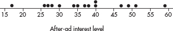
Third, calculate the test statistic t and the P-value: Calculator software (such as T-Test with Data on the TI-84) gives t = 2.526 and P = 0.012113. [For instructional purposes in this review book, we note that = 37.2 and s = 11.04 which gives  and with df = 15 – 1 = 14, P(t > 2.526) = 0.0121.]
Fourth, linking to the P-value, give a conclusion in context: With a P-value this small, 0.0121 < 0.05, there is sufficient evidence to reject H0, that is, there is sufficient evidence to support the ad developer’s claim that after seeing the ad, the mean interest level is above 30.
(b) First, state the hypotheses: H0: µD = 0, Ha: µD ≠ 0, where µD is the mean difference between after-ad and before-ad interest level.
Second, identify the test and check the assumptions: This is a paired t-test, that is, a single sample hypothesis test on the set of differences, and it is given that all assumptions for hypothesis testing are met.
Third, calculate the test statistic t and the P-value: Calculator software (such as T-Test with Data on the TI-84) gives t = 0.9693 and P = 0.174415. [For instructional purposes in this review book, we note that = 0.6667 and s = 2.664 giving t =  and with df = 15 – 1 = 14, P(t > 0.9693) = 0.1744.]
Fourth, linking to the P-value, give a conclusion in context: With a P-value this large, 0.1744 > 0.05, there is not sufficient evidence to reject H0, that is, there is not sufficient evidence that after seeing the ad, teenagers have increased interest in the new website.
(c) A least square regression line using the after-ad and before-ad interest levels has a high correlation of r = 0.972, which when combined with the scatterplot, indicates a strong association. Thus, after-ad interest level can be predicted from before-ad interest level.
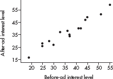
(d) A least square regression line using the before-ad and the change in interest levels yields a very low correlation of r = 0.235, which when combined with the scatterplot, indicates almost no association. Thus, after-ad interest level cannot be predicted from before-ad interest level.
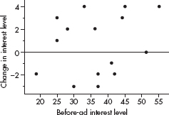
5. (a) One of many ways to proceed: let the digits 1 and 2 represent having a passport, while the remaining single digits represent not having a passport. Read off groups of ten digits, checking for the number of 1s and 2s in each group.
2498346851 4113296825 1485367833 8663018872 7373275392
5062790330 2367029195 4153038298 7360048279 4207598980
9574649262 4488086249 2651769472 9462095309 4072555345
7894788460 2391904958 0201791131 9856022851 1405559336
6003121057 4154811850 7697586849 9644852135 0811348895
Tabulating from the table gives:
No passports (no 1s or 2s): 2
One passport (one 1 or 2): 8
Two passports (two 1s or 2s): 8
Three passports (three 1s or 2s): 5
Four passports (four 1s or 2s): 1
Five passports (five 1s or 2s): 1
The estimated probability of at least three passports among ten 18–24-year-olds is thus 
(b) In a binomial distribution with n = 10 and p = 0.20, P(x 3) = 0.3222. (On the TI-84, 1 - binomcdf(10, 0.20, 2) = 1 – 0.6778 = 0.3222.)
(c) First, state the hypotheses: H0: p = 0.20, Ha: p < 0.20. (If asked to state the parameter, then state “where p is the proportion of all 18–24-year-olds who have passports.”)
Second, identify the test and check the assumptions: This is a one-sample z-test for a population proportion, we have an SRS, np = (200)(0.20) = 40 > 10, n(1 – p) = (200) (0.80) = 160 > 10, and clearly 200 < 10% of all 18–24-year-olds.
Third, calculate the test statistic z and the P-value: Calculator software (such as 1-PropZTest on the TI-84) gives z = –1.2374 and P = 0.107963. [For instructional purposes in this review book, we note that:

Fourth, linking to the P-value, give a conclusion in context. With a P-value this large, 0.1080 > 0.05, there is not sufficient evidence to reject H0, that is, there is not sufficient evidence to dispute the claim that 20% of 18–24-year-olds have passports.
(d) This geometric probability is (0.8)2(0.2) = 0.128.
(e) xP(x) = 1(0.21) + 2(0.15) + 3(0.13) + … + 12(0.02) = 4.31 (On the TI-84, put 1–12 in L1, put the frequencies 21, 15, 13, …, 2 in L2, and then 1-VarStats gives = 4.31.)
6. (a) Normal distributions are symmetric so the mean and median are equal. M = μ = 82.
(b) H0: M = 82, Ha: M > 82
(c) 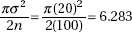
(d) The sampling distribution of the sample median,  , is roughly normal with mean 82 and standard deviation
  p(z > 1.197) and normalcdf(1.197,1000)= 0.1157. [Or normalcdf (85,1000,82,2.507)= 0.1157.] With this large a P-value, 0.1157 > 0.05, there is not sufficient evidence to say that the median number of hours per year that these commuters spend a year sitting in congested traffic is rising.
(e) If n = 200, then 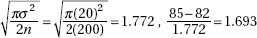 and normalcdf (1.693,1000)= 0.0452. [Or normalcdf(85,1000,82,1.772)= 0.0452.] This does change the conclusion because with this small a P-value, 0.0452 < 0.05, there is sufficient evidence to reject the null hypothesis, that is, there is sufficient evidence to say that the median number of hours per year that these commuters spend a year sitting in congested traffic is rising.
15 Tests of Significance—Chi-Square and Slope of Least Squares Line
Answers Explained
MULTIPLE-CHOICE
1. (C) There are two observations of each mouse, a before time and an after time. These two times are dependent so a paired t-test is appropriate, not a two-sample test.
2. (E) The expected counts if dog bites occur equally during all moon phases are each  (32 + 27 + 47 + 38) = 36. A chi-square goodness-of-fit test gives
  and with df = 4 – 1 = 3, P(2 > 6.167) = 0.1038. With this large a P-value (0.1038 > 0.10), there is not sufficient evidence to conclude that dog bites are related to moon phases.
3. (B) df = (rows – 1)(columns – 1) = (2 – 1)(5 – 1) = 4
4. (C) Picking separate samples from each of 16 populations and classifying according to one variable (perception of quality education) is a survey design which is most appropriately analyzed using a chi-square test of homogeneity of proportions.
5. (D) With 77 + 85 + 23 + 15 = 200 samples, the expected counts if the blood type distribution on the island is the same as that of the general population are 46% of 200 = 92, 40% of 200 = 80, 10% of 200 = 20, and 4% of 200 = 8. A chi-square goodness-of-fit test gives  and with df = 4 – 1 = 3, P(2 > 9.333) = 0.0252. With a P-value this small (0.0252 < 0.05), there is sufficient evidence at the 5% significance level that blood type distribution on the island is different from that of the general population.
6. (D) With df = (3 – 1)(5 – 1) = 8, P(2 > 13.95) = 0.083. Since 0.05 < 0.083 < 0.10, there is evidence at the 10% significance level, but not at the 5% significance level, of a relationship between education level and sports interest.
7. (E) With a P-value this small (less than 0.05), there is evidence in support of the alternative hypothesis Ha: the distributions of music preferences are different, that is, they differ for at least one of the proportions.
8. (D) With 1 + 3 + 3 + 9 = 16, according to the geneticist the expected number of fruit flies of each species is  1125. A chi-square goodness-of-fit test gives

and with df = 4 – 1 = 3, P(2 > 8) = 0.0460. With a P-value this small (0.0460 < 0.05), there is sufficient evidence at the 5% significance level to reject the geneticist’s claim.
9. (E) A chi-square test of independence gives 2 = 2.852, and with df = 2, we find P = 0.2403, and since 0.2403 > 0.10, there is not evidence at the 10% significance level of a relationship between taste preference and the presence of the marker.
10. (E) A chi-square test of homogeneity gives 2 = 5.998, and with df = 3, the P-value is 0.1117. With a P-value this large (0.1117 > 0.10) there is not evidence of a difference in cafeteria food satisfaction among the class levels.
11. (E) The relevant P-value is 0.065 which is less than 0.10 but greater than 0.05.
12. (E) In computer printouts of regression analysis, “S” typically gives the standard deviation of the residuals.
FREE-RESPONSE
1. First, state the hypotheses: H0: The colors of the sugar shells are distributed according to 35% cherry red, 10% vibrant orange, 10% daffodil yellow, 25% emerald green, and 20% royal purple, and Ha: The colors of the sugar shells are not distributed as claimed by the manufacturer. Or [H0: PCR = 0.35, PVO = 0.10, PDY = 0.10, PEG = 0.25, PRP = 0.20, and Ha: at least one proportion is different from this distribution.]
Second, identify the test and check the assumptions: 2 goodness-of-fit test. We are given a random sample, and calculate that all expected cells are at least 5: 35% of 300 = 105, 10% of 300 = 30, 25% of 300 = 75, and 20% of 300 = 60.
Third, calculate the test statistic 2 and the P-value: A calculator gives

Fourth, linking to the P-value, give a conclusion in context: With a P-value this large (0.153 > 0.10), there is not sufficient evidence to reject H0, that is, there is not sufficient evidence that the distribution is different from what is claimed by the manufacturer.
2. (a) Design I, with a single sample from one population classified on two variables (smoking and fitness), will result in a test of independence. Design II, with independent samples from two populations each with the single variable (fitness), will result in a test of homogeneity.
(b) Design II, with its test of homogeneity, and using an equal sample size from each of the two populations (smokers and non-smokers), is best for comparing proportions of smokers who have different fitness levels with proportions of non-smokers who have different fitness levels.
(c) Design I, which classifies one population on the two variables, smoking and fitness, is the only one of these two designs which will give data on the conditional distribution of people with given fitness levels who are smokers or are not smokers.
3. (a) First, state the hypotheses: H0: Happiness level is independent of busy/idle choice for high school students and Ha: Happiness level is not independent of busy/idle choice for high school students.
Second, identify the procedure and check the conditions: This is a chi-square test of independence. It is given that there is a random sample, the data are measured as “counts,” and the expected counts are all at least 5 (put the observed counts in a matrix; then 2-Test on the TI-84 gives expected counts of
|
14.6 |
19.6 |
21.8 |
20.2 |
21.8 |
|
11.4 |
15.4 |
17.2 |
15.8 |
17.2 |
Third, calculate the test statistic and the P-value: Calculator software (2-Test on the TI-84) gives 2 = 14.54 with P = 0.0058 and df = 4.
Fourth, give a conclusion in context with linkage to the P-value: With a P-value this small, 0.0058 < 0.01, there is strong evidence to reject H0, that is, there is strong evidence of a relationship between happiness level and busy/idle choice for high school students.
(b) No, it is not reasonable to conclude that encouraging high school students to keep more busy will lead to higher happiness levels. This was not an experiment with students randomly chosen to sit or walk. The students themselves chose whether or not to sit or walk so no cause-and-effect conclusion is possible. For example, it could well be that the happier students choose to walk, whereas the less happy students choose to sit.
4. (a) First, state the hypotheses: H0: Eating breakfast and morning energy level are independent and Ha: Eating breakfast and morning energy level are not independent.
Second, identify the test and check the assumptions: This is a 2 test of independence on
|
111 |
120 |
120 |
|
60 |
50 |
40 |
where we are given a random sample, and a calculator gives that all expected cells are at least 5:
|
119 |
119 |
112 |
|
51 |
51 |
48 |
Third, calculate the test statistic 2 and the P-value: Calculator software (such as 2-Test on the TI-84) gives 2 = 4.202 and P = 0.1224.
Fourth, linking to the P-value, give a conclusion in context: With this large a P-value, 0.1224 > 0.05, there is not sufficient evidence to reject H0, that is, there is not sufficient evidence of a relationship between eating breakfast and morning energy level.
(b) Yes, the conclusion changes. With n = 1000, the observed numbers are:
|
220 |
240 |
240 |
|
120 |
100 |
80 |
with 2 = 8.403 and P = 0.0150. With a P-value this small (0.0150 < 0.05), now there is sufficient evidence of a relationship between eating breakfast and morning energy level.
5. (a) First, state the hypotheses: H0: The different treatments lead to the same satisfaction levels and Ha: The different treatments lead to different satisfaction levels.
Second, identify the test and check the assumptions: 2 test of homogeneity. We are given a random sample, and a calculator gives that all expected cells are at least 5:
|
55.6 |
55.6 |
27.8 |
|
23.6 |
23.6 |
11.8 |
|
20.8 |
20.8 |
10.4 |
Third, calculate the test statistic 2 and the P-value: A calculator gives 2 = 10.9521, and with df = 4, P = 0.0271.
Fourth, linking to the P-value, give a conclusion in context: With this small a P-value, 0.0271 < 0.05, there is sufficient evidence to reject H0, that is, there is sufficient evidence that the different treatments do lead to different satisfaction levels.
(b) An example of a possible confounding variable is severity of the acne outbreak. It could be that those with more severe cases have less satisfaction no matter what the treatment and are also the ones who are encouraged to use oral medications or laser therapy. So it would be wrong to conclude that oral medications or laser therapy are the causes of less satisfaction.
6. (a) Each additional year in age of teenagers is associated with an average of 0.4577 more texts per waking hour.
(b) The scatterplot of texts per hour versus age should be roughly linear, there should be no apparent pattern in the residual plot, and a histogram of the residuals should be approximately normal.
(c) First, state the hypotheses: H0:  = 0, Ha: ≠ 0, where is the slope of the regression line that relates average texts per hour to age.
Second, identify the test and check the assumptions: This is a test of significance for the slope of the regression line, and we are given that all conditions for inference are met.
Third, calculate the test statistic t and the P-value: The computer printout gives that t = 2.45 and P = 0.016.
Fourth, linking to the P-value, give a conclusion in context: With this small a P-value, 0.016 < 0.05, there is sufficient evidence to reject H0, that is, there is sufficient evidence of a linear relationship between average texts per hour and age for teenagers ages 13–17.
(d) R–Sq = 5.8%, so even though there is evidence of a linear relationship between average texts per hour and age for teenagers ages 13–17, only 5.8% of the variability in average texts per hour is explained by this regression model (or “is accounted for by the variation in age.”).
7. First, state the hypotheses: H0: = 0, Ha: ≠ 0. (If asked to state the parameter, then state “where is the slope of the regression line that relates average fertility rate to women’s life expectancy.”)
Second, identify the test and check the assumptions: This is a test of significance for the slope of the regression line. We are given that the data come from a random sample of countries.
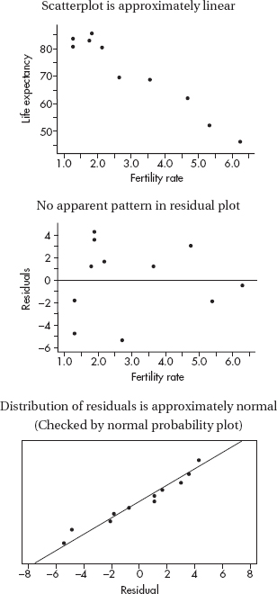
Third, calculate the test statistic t and the P-value: Using a calculator (for example, LinRegTTest on the TI-84) gives that t = –12.53 and P = 0.0000.
Fourth, linking to the P-value, give a conclusion in context: With a P-value this small, 0.0000 < 0.05, there is sufficient evidence to reject H0, that is, there is sufficient evidence of a linear relationship between average fertility rate (children/woman) and life expectancy (women).
INVESTIGATIVE TASK
1. (a) The binomial distribution with p = 0.2 and n = 3 results in: P(0) = (0.8)3 = 0.512, P(1) = 3(0.2)(0.8)2 = 0.384, P(2) = 3(0.2)2(0.8) = 0.096, P(3) = (0.8)3 = 0.008.
(b) Multiplying each of the probabilities in (a) by 800 gives the expected number of occurrences:
|
0 |
1 |
2 |
3 |
|
Expected (if binomial) |
409.6 |
307.2 |
76.8 |
6.4 |
(c) First, state the hypotheses: H0: The number of researchers able to determine the composition of a placebo follows a binomial with p = 0.2 and Ha: The number of researchers able to determine the composition of a placebo does not follow a binomial with p = 0.2.
Second, identify the test and check the assumptions: This is a chi-square test of goodness-of-fit. We must assume that the 800 studies form a representative sample. We note from (b) that all expected cells are 5:
Third, calculate the test statistic 2 and the P-value: A calculator gives 
Fourth, linking to the P-value, give a conclusion in context: With a P-value this small, 0.02549 < 0.05, there is sufficient evidence to reject H0, that is, there is sufficient evidence that the number of researchers able to determine the composition of a placebo does not follow a binomial with p = 0.2.
2. (a) This is a matched-pair t-test on the set of differences {–1.7, –0.2, 1.0, 2.0, 1.3, 0.4, –0.1, 0.4, 0.8, –1.2, 0.4, 0.9}, with H0: µd = 0 and Ha: µd > 0. The sample is random (given), and a dotplot of the differences is roughly unimodal and symmetric (so a normal population distribution is a reasonable assumption):
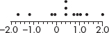
Calculator software (such as T-Test with Data on the TI-84) gives t = 1.121 and P = 0.143. [For instructional purposes in this review book, we note that = 0.3333, 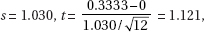 and with df = 12 – 1 = 11, P = 0.143.] With a P-value this large, 0.143 > 0.05, there is not sufficient evidence to reject H0, that is, there is not sufficient evidence that the average student score is greater than that of the English teachers.
(b) This is a matched-pair t-test on the set of differences {–0.3, 1.6, 0.7, 0.3, 0.5, –0.1, –0.8, 0.9, 0.5, –0.1, 0.2, 1.1}, with H0: µd = 0 and Ha: µd > 0. The sample is random (given), and a dotplot of the differences is roughly unimodal and symmetric (so a normal population distribution is a reasonable assumption):
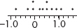
Calculator software (such as T-Test with Data on the TI-84) gives t = 1.974 and P = 0.0370. [For instructional purposes in this review book, we note that = 0.375, 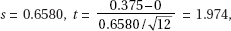 and with df = 12 – 1 = 11, P = 0.037.] With a P-value this small, 0.037 < 0.05, there is sufficient evidence to reject H0, that is, there is sufficient evidence that the average student score is greater than that of the math teachers.
(c) In both regression analyses, the scatterplots are roughly linear and the residual plots show no apparent pattern; however, while 70.1% of the variance in student scores is explained by the variance in math teacher scores, only 27.8% of the variance in student scores is explained by variance in English teacher scores. Thus, the math teacher scores are a better predictor of student scores.
(d) Using the regression equation giving predicted student score as a function of math teacher score gives –0.330 + 1.0701(10.0) = 10.37.
(e) The regression output gives a standard deviation of s = 0.6867. Using the 10.37 estimate from part (d) gives a range of scores for students whose math teachers’ average score is 10.0 to be 10.37 ± 3(0.6867) = 10.37 ± 2.06. Thus, for schools where the math teachers’ average score is 10.0, almost all the average student scores will be between 8.31 and 12.4.
3. (a) The z-scores for 22.5 and 27.5 are, respectively, 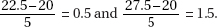 Similarly, 17.5 and 12.5 have z-scores of –0.5 and –1.5, respectively. Using the normal probability table or a calculator gives the probabilities: P(z < –1.5) = 0.0668, P(–1.5 < z < –0.5) = 0.2417, P(–0.5 < z < 0.5) = 0.3830, P(0.5 < z < 1.5) = 0.2417, P(z > 1.5) = 0.0668.
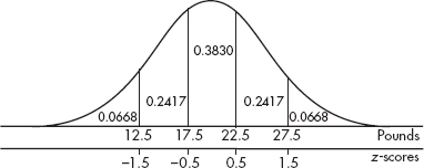
(b) Multiplying each probability by 500: 0.0668(500) = 33.4, 0.2417(500) = 120.85, 0.3830(500) = 191.5, 0.2417(500) = 120.85, and 0.0668(500) = 33.4.
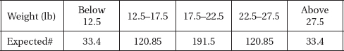
(c) First, state the hypotheses: H0: The weights of student backpacks follow a normal distribution with µ = 20 and = 5 and Ha: The weights of student backpacks do not follow a normal distribution with µ = 20 and = 5.
Second, identify the test and check the assumptions: This is a chi-square test of goodness-of-fit. We are given that the weights are from a random sample of students. We note from above that all expected cells are 5:
Third, calculate the test statistic 2 and the P-value: A calculator gives

Fourth, linking to the P-value, give a conclusion in context: With a P-value this large, 0.1476 > 0.05, there is not sufficient evidence to reject H0, that is, there is not sufficient evidence that the data do not follow a normal distribution with µ = 20 and = 5.