
15 Tests of Significance—Chi-Square and Slope of Least Squares Line
 CHI-SQUARE TEST FOR GOODNESS OF FIT
CHI-SQUARE TEST FOR INDEPENDENCE
CHI-SQUARE TEST FOR HOMOGENEITY OF PROPORTIONS
HYPOTHESIS TEST FOR SLOPE OF LEAST SQUARES LINE
In this topic we continue our development of tools to analyze data. We learn about inference on distributions of counts using chi-square models. This can be used to solve such problems as “Do test results support Mendel’s genetic principles?” (goodness-of-fit test); “Was surviving the Titanic sinking independent of a passenger’s status?” (independence test); and “Do students, teachers, and staff show the same distributions in types of cars driven?” (homogeneity test). We then learn about inference with regard to linear association of two variables. This can be used to solve such problems as “Is there a linear relationship between the grade received on a term paper and the number of pages turned in?”
TIP
Unless you have counts, you cannot use  2 methods.
CHI-SQUARE TEST FOR GOODNESS OF FIT
A critical question is often whether or not an observed pattern of data fits some given distribution. A perfect fit cannot be expected, and so we must look at discrepancies and make judgments as to the goodness of fit.
One approach is similar to that developed earlier. There is the null hypothesis of a good fit, that is, the hypothesis that a given theoretical distribution correctly describes the situation, problem, or activity under consideration. Our observed data consist of one possible sample from a whole universe of possible samples. We ask about the chance of obtaining a sample with the observed discrepancies if the null hypothesis is really true. Finally, if the chance is too small, we reject the null hypothesis and say that the fit is not a good one.
TIP
In Topic 14, the tests were about population parameters; however, with 2, the tests will be about distributions or relationships involving categorical variables.
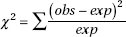
How do we decide about the significance of observed discrepancies? It should come as no surprise that the best information is obtained from squaring the discrepancy values, as this has been our technique for studying variances from the beginning. Furthermore, since, for example, an observed difference of 23 is more significant if the original values are 105 and 128 than if they are 10,602 and 10,625, we must appropriately weight each difference. Such weighting is accomplished by dividing each difference by the expected values. The sum of these weighted differences or discrepancies is called chi-square and is denoted as 2 ( is the lowercase Greek letter chi):
The smaller the resulting 2-value, the better the fit. The P-value is the probability of obtaining a 2 value as extreme or more extreme than the one obtained if the null hypothesis is assumed true. If the 2 value is large enough, that is, if the P-value is small enough, we say there is sufficient evidence to reject the null hypothesis and to claim that the fit is poor.
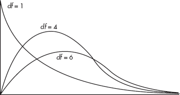
To decide how large a calculated 2-value must be to be significant, that is, to choose a critical value, we must understand how 2-values are distributed. A 2-distribution is not symmetric and is always skewed to the right. There are distinct 2-distributions, each with an associated number of degrees of freedom (df). The larger the df value, the closer the 2-distribution to a normal distribution. Note, for example, that squaring the often-used z-scores 1.645, 1.96, and 2.576 results in 2.71, 3.84, and 6.63, respectively, which are entries found in the first row of the 2-distribution table.
TIP
As long as the observed values do not exactly equal the expected values, 2 ≠ 0, and the explanation is either random chance or that the claimed distribution is incorrect.
A large 2-value may or may not be significant—the answer depends on which 2-distribution we are using. A table is given of critical 2-values for the more commonly used percentages or probabilities. To use the 2-distribution for approximations in goodness-of-fit problems, the individual expected values cannot be too small. An often-used rule of thumb is that no expected value should be less than 5. Finally, as in all hypothesis tests we’ve looked at, the sample should be randomly chosen from the given population.
TIP
In Topic 14, the tests could be one-sided or two-sided; however, with 2, the Ha will always simply be that the H0 is incorrect.
 EXAMPLE 15.1
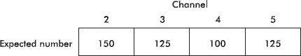
In a recent year, at the 6 p.m. time slot, television channels 2, 3, 4, and 5 captured the entire audience with 30%, 25%, 20%, and 25%, respectively. During the first week of the next season, 500 viewers are interviewed.
a. If viewer preferences have not changed, what number of persons is expected to watch each channel?
Answer: 0.30(500) = 150, 0.25(500) = 125, 0.20(500) = 100, and 0.25(500) = 125, so we have
b. Suppose that the actual observed numbers are as follows:
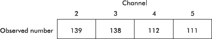
Do these numbers indicate a change? Are the differences significant?
Answer: Check the conditions:
1. Randomization: We must assume that the 500 viewers are a representative sample.
2. We note that the expected values (150, 125, 100, 125) are all  5.
5.
H0: The television audience is distributed over channels 2, 3, 4, and 5 with percentages 30%, 25%, 20%, and 25%, respectively.
Ha: The audience distribution is not 30%, 25%, 20%, and 25%, respectively.
NOTE
We check that the expected values are all ≥ 5.
We calculate
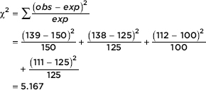
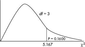
Then the P-value is P = P(2 > 5.167) = 0.1600. [If n is the number of classes, df = n – 1 = 3, and 2cdf(5.167, 1000, 3) = 0.1600.] We also note that putting the observed and expected numbers in Lists, calculator software (such as 2GOF-Test on the TI-84) gives 2 = 5.167 and P = 0.1600.
NOTE
Sometimes it is useful to note which terms in the summation are larger and which are smaller, that is, which terms contribute the most to the final sum.
Conclusion:
With this large a P-value (0.1600) there is not sufficient evidence to reject H0. That is, there is not sufficient evidence that viewer preferences have changed.
Note: While the TI-83 does not have the goodness of fit download that is available on the TI-84, one can still use a TI-83 to calculate the above 2 by putting the observed values in list L1 and the expected values in L2, then calculating (L1 – L2)2/L2 → L3 and 2 = sum(L3), where “sum” is found under LIST → MATH.
TIP
With the t-distribution, the df depends on the sample size, but here, df depends on the number of classes or categories.
EXAMPLE 15.2
TIP
Remember: the hypotheses are always about the population, never about the sample; it would be wrong to say H0: the sample data are uniformly distributed over the five locations.
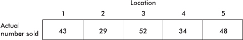
A grocery store manager wishes to determine whether a certain product will sell equally well in any of five locations in the store. Five displays are set up, one in each location, and the resulting numbers of the product sold are noted.
Is there enough evidence that location makes a difference? Test at both the 5% and 10% significance levels.
Answer:
H0: Sales of the product are uniformly distributed over the five locations.
Ha: Sales are not uniformly distributed over the five locations.
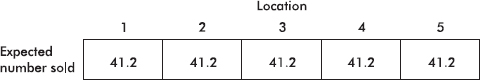
A total of 43 + 29 + 52 + 34 + 48 = 206 units were sold. If location doesn’t matter, we would expect  units sold per location (uniform distribution).
TIP
Even though the observed values are counts and thus integers, the expected values might not be integers and should not be rounded to integers.
Check the conditions:
1. Randomization: We must assume that the 206 units sold are a representative sample.
2. We note that the expected values (all 41.2) are all 5.
Putting the observed and expected numbers in Lists, and with df = 5 – 1 = 4, calculator software (such as 2GOF-Test on the TI-84) gives 2 = 8.903 and P = 0.0636. [For instructional purposes, we note that
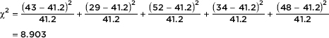
With P = 0.0636 there is sufficient evidence to reject H0 at the 10% level but not at the 5% level. If the grocery store manager is willing to accept a 10% chance of committing a Type I error, there is enough evidence to claim location makes a difference.
CHI-SQUARE TEST FOR INDEPENDENCE
In the goodness-of-fit problems above, a set of expectations was based on an assumption about how the distribution should turn out. We then tested whether an observed sample distribution could reasonably have come from a larger set based on the assumed distribution.
In many real-world problems we want to compare two or more observed samples without any prior assumptions about an expected distribution. In what is called a test of independence, we ask whether the two or more samples might reasonably have come from some larger set. For example, do nonsmokers, light smokers, and heavy smokers all have the same likelihood of being eventually diagnosed with cancer, heart disease, or emphysema? Is there a relationship (association) between smoking status and being diagnosed with one of these diseases?
We classify our observations in two ways and then ask whether the two ways are independent of each other. For example, we might consider several age groups and within each group ask how many employees show various levels of job satisfaction. The null hypothesis is that age and job satisfaction are independent, that is, that the proportion of employees expressing a given level of job satisfaction is the same no matter which age group is considered.
Analysis involves calculating a table of expected values, assuming the null hypothesis about independence is true. We then compare these expected values with the observed values and ask whether the differences are reasonable if H0 is true. The significance of the differences is gauged by the same 2-value of weighted squared differences. The smaller the resulting 2-value, the more reasonable the null hypothesis of independence. If the 2-value is large enough, that is, if the P-value is small enough, we can say that the evidence is sufficient to reject the null hypothesis and to claim that there is some relationship between the two variables or methods of classification.
In this type of problem,
df = (r – 1) (c – 1)
where df is the number of degrees of freedom, r is the number of rows, and c is the number of columns.
A point worth noting is that even if there is sufficient evidence to reject the null hypothesis of independence, we cannot necessarily claim any direct causal relationship. In other words, although we can make a statement about some link or relationship between two variables, we are not justified in claiming that one causes the other. For example, we may demonstrate a relationship between salary level and job satisfaction, but our methods would not show that higher salaries cause higher job satisfaction. Perhaps an employee’s higher job satisfaction impresses his superiors and thus leads to larger increases in pay. Or perhaps there is a third variable, such as training, education, or personality, that has a direct causal relationship to both salary level and job satisfaction.
EXAMPLE 15.3
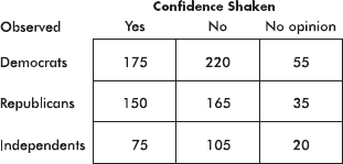
In a nationwide telephone poll of 1000 randomly selected adults representing Democrats, Republicans, and Independents, respondents were asked two questions: their party affiliation and if their confidence in the U.S. banking system had been shaken by the savings and loan crisis. The answers, cross-classified by party affiliation, are given in the following contingency table.
Test the null hypothesis that shaken confidence in the banking system is independent of party affiliation. Use a 10% significance level.
Answer:
H0: Party affiliation and shaken confidence in the banking system are independent.
Ha: Party affiliation and shaken confidence in the banking system are not independent.
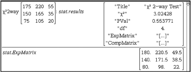
Putting the observed data into a Matrix, calculator software (such as 2-Test on the TI-84) gives 2 = 3.024 and P = 0.5538, and stores the expected values in a second matrix:
We are given a random sample and note that all expected cells are 5.
TIP
It is not enough to just say that all expected cells are ≥ 5; you must list the expected counts.
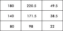
With this large a P-value, 0.5538 > 0.05, there is not sufficient evidence to reject H0, that is, there is not sufficient evidence of any relationship between party affiliation and shaken confidence in the banking system. For instructional purposes, we note that the expected values, 2, and P can be calculated as follows:
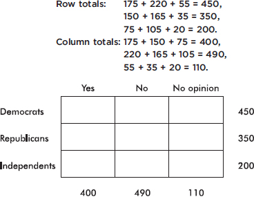
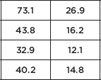
To calculate, for example, the expected value in the upper left box, we can proceed in any of several equivalent ways. First, we could note that the proportion of Democrats is  and so, if independent, the expected number of Democrat yes responses is 0.45(400) = 180. Instead, we could note that the proportion of yes responses is
  and so, if independent, the expected number of Democrat yes responses is 0.4(450) = 180. Finally, we could note that both these calculations simply involve
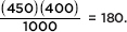
In other words, the expected value of any box can be calculated by multiplying the corresponding row total by the appropriate column total and then dividing by the grand total. Thus, for example, the expected value for the middle box, which corresponds to Republican no responses, is 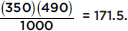
Continuing in this manner, we fill in the table as follows:
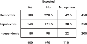
[An appropriate check at this point is that each expected cell count is at least 5.]
Next we calculate the value of chi-square:
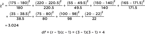
P is then calculated using calculator software such as 2cdf(3.024, 1000, 4) of the TI-84.] On the TI-Nspire the result shows as:
As for conditions to check for chi-square tests for independence, we should check that the sample is randomly chosen and that the expected values for all cells are at least 5. If a category has one of its expected cell count less than 5, we can combine categories that are logically similar (for example “disagree” and “strongly disagree”), or combine numerically small categories collectively as “other.”
EXAMPLE 15.4
To determine whether men with a combination of childhood abuse and a certain abnormal gene are more likely to commit violent crimes, a study is run on a simple random sample of 575 males in the 25 to 35 age group. The data are summarized in the following table:
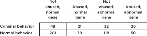
a. Is there evidence of a relationship between the four categories (based on childhood abuse and abnormal genetics) and behavior (criminal versus normal)? Explain.
b. Is there evidence that among men with the normal gene, the proportion of abused men who commit violent crimes is greater than the proportion of nonabused men who commit violent crimes? Explain.
c. Is there evidence that among men who were not abused as children, the proportion of men with the abnormal gene who commit violent crimes is greater than the proportion of men with the normal gene who commit violent crimes? Explain.
d. Is there a contradiction in the above results? Explain.
Answers:
a. A chi-square test for independence is indicated. The expected cell counts are as follows:
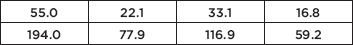
The condition that all cell counts are greater than 5 is met.
H0: The four categories (based on childhood abuse and abnormal genetics) and behavior (criminal versus normal) are independent.
Ha: The four categories (based on childhood abuse and abnormal genetics) and behavior (criminal versus normal) are not independent (there is a relationship).
Running a chi-square test gives 2 = 7.752. With df = (r – 1)(c – 1) = 3, we get P = 0.0514. Since 0.0514 < 0.10, the data do provide some evidence (at least at the 10% significance level) to reject H0 and conclude that there is evidence of a relationship between the four categories (based on childhood abuse and abnormal genetics) and behavior (criminal versus normal).
b. A two-proportion z-test is indicated. We must check that n is large enough: n1 1 = 21 10, n1(1 – 1) = 79 10, n22 = 48 10, n2(1 – 2) = 201 10. We are given SRSs that are less than 10% of all males in the 25 to 35 age group.
H0: p1 – p2 = 0 |
(where p1 is the proportion of abused men with normal genetics who commit violent crimes and p2 is the proportion of nonabused men with normal genetics who commit violent crimes) |
Ha: p1 – p2 > 0 |
(the proportion of abused men with normal genetics who commit violent crimes is greater than the proportion of nonabused men with normal genetics who commit violent crimes) |
Calculator software (such as 2-PropZTest on the TI-84) gives z = 0.3653 and P = 0.3574. With this large a P-value, 0.3574 > 0.05, there is not sufficient evidence to reject H0, that is, there is not sufficient evidence that the proportion of abused men with normal genetics who commit violent crimes is greater than the proportion of nonabused men with normal genetics who commit violent crimes.
c. A two-proportion z-test is indicated. We must check that n is large enough: n11 = 32 10, n1(1 – 1) = 118 10, n22 = 48 10, n2(1 – 2) = 201 10. We are given SRSs that are less than 10% of all males in the 25 to 35 age group.
H0: p1 – p2 = 0 |
(where p1 is the proportion of nonabused men with abnormal genetics who commit violent crimes and p2 is the proportion of nonabused men with normal genetics who commit violent crimes) |
Ha: p1 – p2 > 0 |
(the proportion of nonabused men with abnormal genetics who commit violent crimes is greater than the proportion of nonabused men with normal genetics who commit violent crimes) |
Calculator software (such as 2-PropZTest on the TI-84) gives z = 0.4969 and P = 0.3096. With this large a P-value, 0.3096 > 0.05, there is not sufficient evidence to reject H0, that is, there is not sufficient evidence that the proportion of nonabused men with the abnormal gene who commit violent crimes is greater than the proportion of nonabused men with the normal gene who commit violent crimes.
d. There is no contradiction. It is possible to have evidence of an overall relationship without significant evidence showing in a subset of the categories.
CHI-SQUARE TEST FOR HOMOGENEITY OF PROPORTIONS
In chi-square goodness-of-fit tests we work with a single variable in comparing a single sample to a population model. In chi-square independence tests we work with a single sample classified on two variables. Chi-square procedures can also be used with a single variable to compare samples from two or more populations. It is important that the samples be simple random samples, that they be taken independently of each other, that the original populations be large compared to the sample sizes, and that the expected values for all cells be at least 5. The contingency table used has a row for each sample.
EXAMPLE 15.5
In a large city, a group of AP Statistics students work together on a project to determine which group of school employees has the greatest proportion who are satisfied with their jobs. In independent simple random samples of 100 teachers, 60 administrators, 45 custodians, and 55 secretaries, the numbers satisfied with their jobs were found to be 82, 38, 34, and 36, respectively. Is there evidence that the proportion of employees satisfied with their jobs is different in different school system job categories?
Answer:
H0: The proportion of employees satisfied with their jobs is the same across the various school system job categories.
Ha: At least two of the job categories differ in the proportion of employees satisfied with their jobs.
The observed counts are as follows:

Putting the observed data into a matrix, calculator software (such as 2-Test on the TI-84) gives 2 = 8.707 and P = 0.0335, and stores the expected values in a second matrix:
We are given an SRS and note that all expected cells are 5. With this small a P-value, 0.0335 < 0.05, there is sufficient evidence to reject H0, that is, there is sufficient evidence that the proportion of employees satisfied with their jobs is not the same across all the school system job categories.
The difference between the test for independence and the test for homogeneity can be confusing. When we’re simply given a two-way table, it’s not obvious which test is being performed. The crucial difference is in the design of the study. Did we pick samples from each of two or more populations to compare the distribution of some variable among the different populations? If so, we are doing a test for homogeneity. Did we pick one sample from a single population and cross-categorize on two variables to see if there is an association between the variables? If so, we are doing a test for independence.
For example, if we separately sample Democrats, Republicans, and Independents to determine whether they are for, against, or have no opinion with regard to stem cell research (several samples, one variable), then we do a test for homogeneity with a null hypothesis that the distribution of opinions on stem cell research is the same among Democrats, Republicans, and Independents. However, if we sample the general population, noting the political preference and opinions on stem cell research of the respondents (one sample, two variables), then we do a test for independence with a null hypothesis that political preference is independent of opinion on stem cell research.
Finally, it should be remembered that while we used 2 for categorical data, the 2 distribution is a continuous distribution, and applying it to counting data is just an approximation.
HYPOTHESIS TEST FOR SLOPE OF LEAST SQUARES LINE
In addition to finding a confidence interval for the true slope, one can also perform a hypothesis test for the value of the slope. Often one uses the null hypothesis H0:  = 0, that is, that there is no linear relationship between the two variables. Assumptions for inference for the slope of the least squares line include the following: (1) the sample must be randomly selected; (2) the scatterplot should be approximately linear; (3) there should be no apparent pattern in the residuals plot; and (4) the distribution of the residuals should be approximately normal. (This third point can be checked by a histogram, dotplot, stemplot, or normal probability plot of the residuals.)
TIP
Be careful about abbreviations. For example, your teacher might use LOBF (line of best fit), but the grader may have no idea what this refers to.
Note that a low P-value tells us that if the two variables did not have some linear relationship, it would be highly unlikely to find such a random sample; however, strong evidence that there is some association does not mean the association is strong.
EXAMPLE 15.6
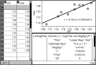
The following table gives serving speeds in mph (using a flat or “cannonball” serve) of ten randomly selected professional tennis players before and after using a newly developed tennis racquet.
TIP
If the data don’t look straight, do not fit a straight line.

a. Is there evidence of a straight line relationship with positive slope between serving speeds of professionals using their old and the new racquets?
Answer: Checking the assumptions:
We are told that the data come from a random sample of professional players.
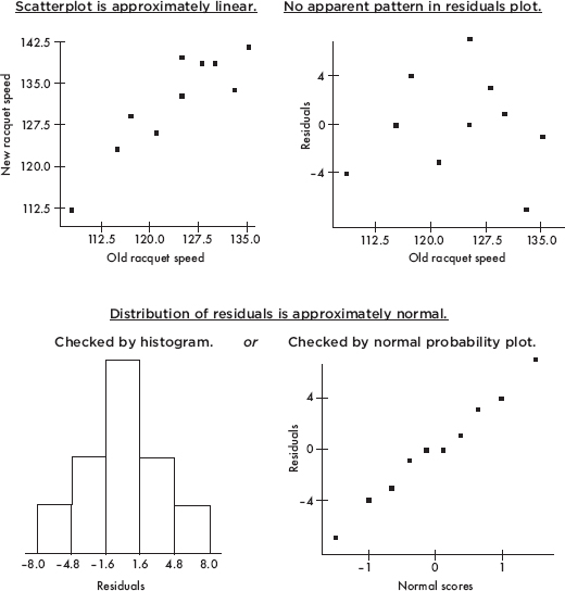
NOTE
A normal probability plot roughly showing a straight line indicates that the data distribution is roughly normal.
We proceed with the hypothesis test for the slope of the regression line.
H0: 1 = 0 Ha: 1 > 0
Using the statistics software on a calculator (for example, LinRegTTest on the TI-84), gives:

With such a small P value, 0.00019 < 0.001, there is very strong evidence to reject H0, that is, there is very strong evidence of a straight line relationship with positive slope between serving speeds of professionals using their old and the new racquets.
b. Interpret in context the least squares line.
Answer: With a slope of approximately 1 and a y-intercept of 8.76, the regression line indicates that use of the new racquet increases serving speed on the average by 8.76 mph regardless of the old racquet speed. That is, players with lower and higher old racquet speeds experience on the average the same numerical (rather than percentage) increase when using the new racquet.
On the TI-Nspire the result shows as:
It is important to be able to interpret computer output, and appropriate computer output is helpful in checking the assumptions for inference.
EXAMPLE 15.7
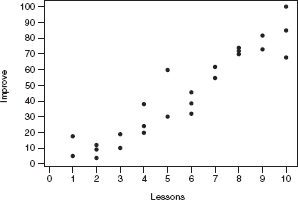
A company offers a 10-lesson program of study to improve students’ SAT scores. A survey is made of a random sampling of 25 students. A scatterplot of improvement in total (math + verbal) SAT score versus number of lessons taken is as follows:
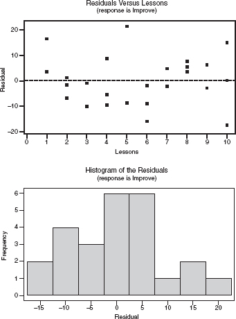
Some computer output of the regression analysis follows, along with a plot and a histogram of the residuals.
Regression Analysis: Improvement Versus Lessons
Dependentvariable:Improvement
Predictor |
Coef |
SE Coef |
T |
P |
Constant |
–7.718 |
4.272 |
–1.81 |
0.084 |
Lessons |
9.2854 |
0.6789 |
13.68 |
0.000 |
S = 9.744R–Sq = 89.1%
Analysis of Variance
Source |
DF |
SS |
MS |
F |
P |
Regression |
1 |
17761 |
17761 |
187.06 |
0.000 |
Residual Error |
23 |
2184 |
95 |
|
|
Total |
24 |
19945 |
|
|
|
a. What is the equation of the regression line that predicts score improvement as a function of number of lessons?
b. Interpret, in context, the slope of the regression line.
c. What is the meaning of R–Sq in context of this study?
d. Give the value of the correlation coefficient.
e. Perform a test of significance for the slope of the regression line.
Answers:
a. 
b. The slope of the regression line is 9.2854, meaning that on the average, each additional lesson is predicted to improve one’s total SAT score by 9.2854.
c. R–Sq = 89.1% means that 89.1% of the variation in total SAT score improvement can be explained by variation in the number of lessons taken.
d. 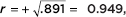 where the sign is positive because the slope is positive.
e. A test of significance of the slope of the regression line with H0: = 0, Ha: ≠ 0 (test of significance of correlation) is as follows:
Assumptions: We are told the data came from a random sample, the scatterplot appears to be approximately linear, there is no apparent pattern in the residuals plot, and the histogram of residuals appears to be approximately normal.

(Or t and P can simply be read off the computer output!)
With this small a P-value, 0.000 < any reasonable significance level, there is very strong evidence to reject H0 and conclude that the relationship between improvement in total SAT score and number of lessons taken is significant.
Throughout this review book the concept of independence has arisen many times, with different meanings in different contexts, and a quick review is worthwhile.
1. If the outcome of one event, E, doesn’t affect the outcome of another event, F, we say the events are independent, and we have P(E |F) = P(E), P(F |E) = P(F), and P(E  F) = P(E)P(F).
2. When the distribution of one variable in a contingency table is the same for all categories of another variable, we say the two variables are independent.
3. When two random variables are independent, we can use the rule for adding variances with regard to the random variables X + Y and X – Y.
4. In a binomial distribution, the trials must be independent; that is, the probability of success must be the same on every trial, irrespective of what happened on a previous trial. However, when we pick a sample from a population, we do change the size and makeup of the remaining population. We typically allow this as long as the sample is not too large—the usual rule of thumb is that the sample size should be smaller than 10% of the population.
5. In inference we wish to make conclusions about a population parameter by analyzing a sample. A crucial assumption is always that the sampled values are independent of each other. This typically involves checking if there was proper randomization in the gathering of data. Also, to minimize the effect on independence from samples being drawn without replacement, we check that less than 10% of the population is sampled.
6. Furthermore, if inference involves the comparison of two groups, the two groups must be independent of each other.
7. With paired data, while the observations in each pair are not independent, the differences must be independent of each other.
8. With regression, the errors in the regression model must be independent, and one may check this by confirming there are no patterns in the residual plot.
SUMMARY
 Chi-square analysis is an important tool for inference on distributions of counts.
The chi-square statistic is found by summing the weighted squared differences between observed and expected counts.
A chi-square goodness-of-fit test compares an observed distribution to some expected distribution.
A chi-square test of independence tests for evidence of an association between two categorical variables from a single sample.
A chi-square test of homogeneity compares samples from two or more populations with regard to a single categorical variable.
The sampling distribution for the slope of a regression line can be modeled by a t-distribution with df = n – 2.
QUESTIONS ON TOPIC FIFTEEN: TESTS OF SIGNIFICANCE—CHI-SQUARE AND SLOPE OF LEAST SQUARES LINE
Multiple-Choice Questions
Directions: The questions or incomplete statements that follow are each followed by five suggested answers or completions. Choose the response that best answers the question or completes the statement.
1. A random sample of mice is obtained, and each mouse is timed as it moves through a maze to a reward treat at the end. After several days of training, each mouse is timed again. The data should be analyzed using
(A) a z-test of proportions.
(B) a two-sample test of means.
(C) a paired t-test.
(D) a chi-square test.
(E) a regression analysis.
2. To test the claim that dogs bite more or less depending upon the phase of the moon, a university hospital counts admissions for dog bites and classifies with moon phase.
|
New moon |
First quarter |
Full moon |
Last quarter |
|
Dog bite admissions |
32 |
27 |
47 |
38 |
Which of the following is the proper conclusion?
(A) The data prove that dog bites occur equally during all moon phases.
(B) The data prove that dog bites do not occur equally during all moon phases.
(C) The data give evidence that dog bites occur equally during all moon phases.
(D) The data give evidence that dog bites do not occur equally during all moon phases.
(E) The data do not give sufficient evidence to conclude that dog bites are related to moon phases.
3. For a project, a student randomly picks 100 fellow AP Statistics students to survey on whether each has either a PC or Apple at home (all students in the school have a home computer) and what score (1, 2, 3, 4, 5) each expects to receive on the AP exam. A chi-square test of independence results in a test statistic of 8. How many degrees of freedom are there?
(A) 1
(B) 4
(C) 7
(D) 9
(E) 99
4. A random sample of 100 former student-athletes are picked from each of the 16 colleges that are members of the Big East conference. Students are surveyed about whether or not they feel they received a quality education while participating in varsity athletics. A 2 × 16 table of counts is generated. Which of the following is the most appropriate test to determine whether there is a difference among these schools as to the student-athlete perception of having received a quality education.
(A) A chi-square goodness-of-fit test for a uniform distribution
(B) A chi-square test of independence
(C) A chi-square test of homogeneity of proportions
(D) A multiple-sample z-test of proportions
(E) A multiple-population z-test of proportions
5. According to theory, blood types in the general population occur in the following proportions: 46% O, 40% A, 10% B, and 4% AB. Anthropologists come upon a previously unknown civilization living on a remote island. A random sampling of blood types yields the following counts: 77 O, 85 A, 23 B, and 15 AB. Is there sufficient evidence to conclude that the distribution of blood types found among the island population differs from that which occurs in the general population?
(A) The data prove that blood type distribution on the island is different from that of the general population.
(B) The data prove that blood type distribution on the island is not different from that of the general population.
(C) The data give evidence at the 1% significance level that blood type distribution on the island is different from that of the general population.
(D) The data give evidence at the 5% significance level, but not at the 1% significance level, that blood type distribution on the island is different from that of the general population.
(E) The data do not give evidence at the 5% significance level that blood type distribution on the island is different from that of the general population.
6. Is there a relationship between education level and sports interest? A study cross-classified 1500 randomly selected adults in three categories of education level (not a high school graduate, high school graduate, and college graduate) and five categories of major sports interest (baseball, basketball, football, hockey, and tennis). The 2-value is 13.95. Is there evidence of a relationship between education level and sports interest?
(A) The data prove there is a relationship between education level and sports interest.
(B) The evidence points to a cause-and-effect relationship between education and sports interest.
(C) There is evidence at the 5% significance level of a relationship between education level and sports interest.
(D) There is evidence at the 10% significance level, but not at the 5% significance level, of a relationship between education level and sports interest.
(E) The P-value is greater than 0.10, so there is no evidence of a relationship between education level and sports interest.
7. A disc jockey wants to determine whether middle school students and high school students have similar music tastes. Independent random samples are taken from each group, and each person is asked whether he/she prefers hip-hop, pop, or alternative. A chi-square test of homogeneity of proportions is performed, and the resulting P-value is below 0.05. Which of the following is a proper conclusion?
(A) There is evidence that for all three music choices the proportion of middle school students who prefer each choice is equal to the corresponding proportion of high school students.
(B) There is evidence that the proportion of middle school students who prefer hip-hop is different from the proportion of high school students who prefer hip-hop.
(C) There is evidence that for all three music choices the proportion of middle school students who prefer each choice is different from the corresponding proportion of high school students.
(D) There is evidence that for at least one of the three music choices the proportion of middle school students who prefer that choice is equal to the corresponding proportion of high school students.
(E) There is evidence that for at least one of the three music choices the proportion of middle school students who prefer that choice is different from the corresponding proportion of high school students.
8. A geneticist claims that four species of fruit flies should appear in the ratio 1:3:3:9. Suppose that a sample of 2000 flies contained 110, 345, 360, and 1185 flies of each species, respectively. Is there sufficient evidence to reject the geneticist’s claim?
(A) The data prove the geneticist’s claim.
(B) The data prove the geneticist’s claim is false.
(C) The data do not give sufficient evidence to reject the geneticist’s claim.
(D) The data give sufficient evidence to reject the geneticist’s claim.
(E) The evidence from this data is inconclusive.
9. A food biologist surveys people at an ice cream parlor, noting their taste preferences and cross-classifying against the presence or absence of a particular marker in a saliva swab test.
|
Presence |
Absence |
|
Vanilla |
32 |
12 |
|
Chocolate |
15 |
7 |
|
Strawberry |
24 |
19 |
Is there evidence of a relationship between taste preference and the marker presence?
(A) At the 10% significance level, the data prove that there is a relationship between taste preference and the presence of the marker.
(B) At the 10% significance level, the data prove that there is no relationship between taste preference and the presence of the marker.
(C) There is evidence at the 5% significance level of a relationship between taste preference and the presence of the marker.
(D) There is evidence at the 10% significance level, but not at the 5% significance level, of a relationship between taste preference and the presence of the marker.
(E) There is no evidence at the 10% significance level of a relationship between taste preference and the presence of the marker.
10. Random samples of 25 students are chosen from each high school class level, students are asked whether or not they are satisfied with the school cafeteria food, and the results are summarized in the following table:
|
Freshmen |
Sophomores |
Juniors |
Seniors |
|
Satisfied |
15 |
12 |
9 |
7 |
|
Dissatisfied |
10 |
13 |
16 |
18 |
Is there evidence of a difference in cafeteria food satisfaction among the class levels?
(A) The data prove that there is a difference in cafeteria food satisfaction among the class levels.
(B) There is evidence of a linear relationship between food satisfaction and class level.
(C) There is evidence at the 1% significance level of a difference in cafeteria food satisfaction among the class levels.
(D) There is evidence at the 5% significance level, but not at the 1% significance level, of a difference in cafeteria food satisfaction among the class levels.
(E) With P = 0.1117 there is no evidence of a difference in cafeteria food satisfaction among the class levels.
11. Can dress size be predicted from a woman’s height? In a random sample of 20 female high school students, dress size versus height (cm) gives the following regression results:
The regression equation is
Size = –48.8 + 0.374 Height
Predictor |
Coef |
SE Coef |
T |
P |
Constant |
–48.81 |
30.57 |
–1.60 |
0.128 |
Height |
0.3736 |
0.1898 |
1.97 |
0.065 |
S = 4.46720R–Sq = 17.7%R–Sq(adj) = 13.1%
Is there statistical evidence of a linear relationship between dress size and height?
(A) No, because r2, the coefficient of determination, is too small.
(B) No, because 0.128 is above any reasonable significance level.
(C) Yes, because by any reasonable observation, taller women tend to have larger dress sizes.
(D) Yes, because the computer printout does give a regression equation.
(E) There is evidence at the 10% significance level, but not at the 5% level.
12. To study the relationship between calories (kcal) and fat (g) in pizza, slices of 14 randomly selected major brand pizzas are chemically analyzed. Computer printout for regression:
Predictor |
Coef |
SE Coef |
T |
P |
Constant |
1.593 |
1.422 |
1.12 |
0.285 |
Calories |
0.035881 |
0.004896 |
7.33 |
0.000 |
S = 1.27515R–Sq = 81.7%R–Sq(adj) = 80.2%
What is measured by S = 1.27515?
(A) Variability in calories among slices
(B) Variability in fat among slices
(C) Variability in the slope (g/kcal) of the regression line
(D) Variability in the y-intercept of the regression line
(E) Variability in the residuals
Free-Reponse Questions
Directions: You must show all work and indicate the methods you use. You will be graded on the correctness of your methods and on the accuracy of your final answers.
SEVEN OPEN-ENDED QUESTIONS
1. A candy manufacturer advertises that their fruit-flavored sweets have hard sugar shells in five colors with the following distribution: 35% cherry red, 10% vibrant orange, 10% daffodil yellow, 25% emerald green, and 20% royal purple. A random sample of 300 sweets yielded the counts in the following table:
|
Cherry |
Vibrant |
Daffodil |
Emerald |
Royal |
|
red |
orange |
yellow |
green |
purple |
|
Observed counts |
94 |
34 |
22 |
77 |
73 |
Is there evidence that the distribution is different from what is claimed by the manufacturer?
2. You want to study whether smokers and non-smokers have equal fitness levels (low, medium, high) and are considering two survey designs:
I. Take a random sample of 200 people, asking each whether or not they smoke, and measuring the fitness level of each.
II. Take a random sample of 100 smokers and measure the fitness level of each, and take a random sample of 100 non-smokers and measure the fitness level of each.
(a) Which of the designs results in a test of independence and which results in a test of homogeneity? Explain.
(b) If we are interested in whether the proportion of people who have various fitness levels differs among smokers and non-smokers, which design should be used? Explain.
(c) If we are interested in the conditional distribution of people with given fitness levels who are smokers or are not smokers, which design should be used? Explain.
3. Is there a difference in happiness levels between busy and idle people? In one study, after filling out a survey, 175 randomly chosen high school students were told they could either sit 15 minutes while the survey was being tabulated, or they could walk 15 minutes to another building where the survey was being tabulated. Then they were given a questionnaire asking how good they felt during the past 15 minutes (on a scale of 1, “not good,” to 5, “very good”). The results of the questionnaire were as follows:
|
Happiness level |
||||
|
1 |
2 |
3 |
4 |
5 |
|
Busy (walking) |
8 |
15 |
24 |
26 |
25 |
|
Idle (sitting) |
18 |
20 |
15 |
10 |
14 |
(a) Does the above data give statistical evidence of a relationship between happiness level and busy/idle choice of the students?
(b) If the answer above is positive for a relationship, is it reasonable to conclude that encouraging high school students to keep more busy will lead to higher happiness levels?
4. A poll, asking a random sample of adults whether or not they eat breakfast and to rate their morning energy level, results in the table:
|
Morning energy level |
||
|
Low |
Medium |
High |
|
Breakfast |
22% |
24% |
24% |
|
No breakfast |
12% |
10% |
8% |
(a) If the sample size was n = 500, is there evidence of a relationship between eating breakfast and morning energy level?
(b) Does the answer to part (a) change if n = 1000 instead? Explain.
5. A survey on acne treatments randomly selected 100 teenagers using topical treatments, 100 using oral medications, and 50 using laser therapy, and asked each subject about satisfaction level. The resulting counts were:
|
Topical |
Oral |
Laser |
|
Very satisfied |
61 |
54 |
24 |
|
Somewhat satisfied |
28 |
21 |
10 |
|
Unsatisfied |
11 |
25 |
16 |
(a) Do the different treatments lead to different satisfaction levels? Perform an appropriate hypothesis test.
(b) What is a possible confounding variable which could lead you to jump to a misleading conclusion? Explain.
6. A study of 100 randomly selected teenagers, ages 13–17, looked at number of texts per waking hour versus age, yielding the computer regression output below:
Predictor |
Coef |
SE Coef |
T |
P |
Constant |
–1.055 |
2.815 |
–0.37 |
0.709 |
Age |
0.4577 |
0.1866 |
2.45 |
0.016 |
S = 2.66501R–Sq = 5.8%R–Sq(adj) = 4.8%
(a) Interpret the slope in context.
(b) What three graphs should be checked with regard to conditions for a test of significance for the slope of the regression line?
(c) Assuming all conditions for inference are met, perform this test of significance.
(d) Give a conclusion in context, taking into account both your answer to the hypothesis test as well as the value of R–Sq.
7. Can the average women’s life expectancy in a country be predicted from the average fertility rate (children/woman) in that country? Following are the most recent data from 11 randomly selected countries:
|
Country |
Fertility rate (children/woman) |
Life expectancy (women) |
|
Afghanistan |
6.25 |
45.5 |
|
Angola |
5.33 |
51.4 |
|
Argentina |
2.16 |
80.0 |
|
Australia |
1.85 |
84.4 |
|
France |
1.85 |
85.1 |
|
Liberia |
4.69 |
61.5 |
|
Nepal |
2.66 |
69.0 |
|
Netherlands |
1.77 |
82.6 |
|
Pakistan |
3.58 |
68.3 |
|
Poland |
1.29 |
80.4 |
|
Singapore |
1.29 |
83.4 |
Perform a test of significance for the slope of the regression line that relates fertility rate (children/woman) to life expectancy (women).
THREE INVESTIGATIVE TASKS
1. Use of placebos are now the norm for medical studies, but disclosing the compositions of these placebos is unexplicitly not all that common, even though these placebos could have effects. For example, olive oil has been used as a placebo in cholesterol drug tests, and there is some evidence that olive oil can affect cholesterol level. Composition of a placebo injection is disclosed more often than that of a placebo pill, but still it can be difficult to make this finding. In a survey of 800 studies using placebo injections, three researchers independently try to determine the compositions of the placebos, and the counts of successes are as follows:
|
Number of researchers able to determine composition of a placebo |
|||
|
0 |
1 |
2 |
3 |
|
|
Number of studies |
419 |
314 |
56 |
11 |
(a) Find the complete binomial distribution (probabilities of 0 through 3 successes) for n = 3 and p = 0.2.
(b) Given 800 studies, if the number of researchers who determine composition of a placebo follows a binomial with probability of success p = 0.2, what are the expected values for the numbers (0 through 3) of researchers able to determine composition of a placebo?
(c) Test the null hypothesis that the number of researchers who determine composition of a placebo follows a binomial with probability of success p = 0.2.
2. Twelve high schools are randomly selected, and in each, the math teachers, the English teachers, and the students on the honor roll all take a logic puzzle test, and average scores for each group are noted in the following table:
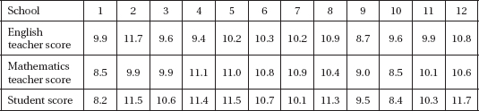
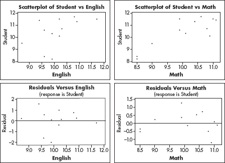
The regression analysis of the data follows.
Regression Analysis: Student versus English
Dependent variable: Student
Predictor |
Coef |
SE Coef |
T |
P |
Constant |
2.315 |
4.154 |
0.56 |
0.590 |
English |
0.8038 |
0.4102 |
1.96 |
0.078 |
S = 1.06798R–Sq = 27.8%R–Sq(adj) = 20.5%
Regression Analysis: Student versus Math
Dependent variable: Student
Predictor |
Coef |
SE Coef |
T |
P |
Constant |
–0.330 |
2.230 |
–0.15 |
0.885 |
Math |
1.0701 |
0.2208 |
4.85 |
0.001 |
S = 0.686661R–Sq = 70.1%R–Sq(adj) = 67.1%
(a) Is there evidence that the average student score is greater than that of the English teachers?
(b) Is there evidence that the average student score is greater than that of the math teachers?
(c) Is the score of the English or math teachers a better predictor of the student score? Explain.
(d) Given the analysis in part (c), predict the average student score in a school where the average English teachers’ score is 11.0 and the average math teachers’ score is 10.0.
(e) Given the analysis in parts (c) and (d), what is the approximate range of average student scores at schools where the average English teachers’ score is 11.0 and the average math teachers’ score is 10.0.
3. A heavy backpack can cause chronic shoulder, neck, and back pain. Wide, padded shoulder straps, a waist belt, and avoidance of single-strap bags all help, but weight is the main problem. The recommendation for a safe weight for school backpacks is no more than 10% of body weight. In a study of 500 randomly selected high school students, the weights of their backpacks give rise to the following:
|
Weight (lb) |
Below 12.5 |
12.5–17.5 |
17.5–22.5 |
22.5–27.5 |
Above 27.5 |
|
Observed # |
28 |
134 |
182 |
112 |
44 |
(a) In a normal distribution with µ = 20 and  = 5, what are the probabilities of z < 12.5, 12.5 < z < 17.5, 17.5 < z < 22.5, 22.5 < z < 27.5, and z > 27.5?
(b) Given 500 students, if the data follow a normal distribution with µ = 20 and = 5, what are the expected values for the numbers of backpacks in each of the indicated weight ranges?
(c) Test the null hypothesis that the data follow a normal distribution with µ = 20 and = 5.