
 PROPERTIES
USING TABLES
A MODEL FOR MEASUREMENT
COMMONLY USED PROBABILITIES AND Z-SCORES
FINDING MEANS AND STANDARD DEVIATIONS
NORMAL APPROXIMATION TO THE BINOMIAL
CHECKING NORMALITY
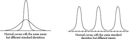
Some of the most useful probability distributions are symmetric and bell-shaped:
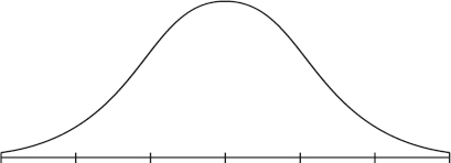
In this topic we study one such distribution called the normal distribution (not all symmetric, unimodal distributions are normal). The normal distribution is valuable in describing various natural phenomena, especially those involving growth or decay. However, the real importance of the normal distribution in statistics is that it can be used to describe the results of sampling procedures.
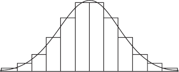
The normal distribution can be viewed as a limiting case of the binomial. More specifically, we start with any fixed probability of success p and consider what happens as n becomes arbitrarily large. To obtain a visual representation of the limit, we draw histograms using an increasingly large n for each fixed p.
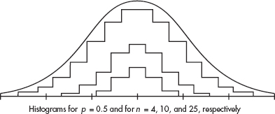
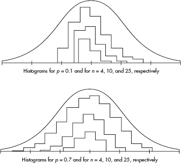
For greater clarity, different scales have been used for the histograms associated with different values of n. From the diagrams above it is reasonable to accept that as n becomes larger without bound, the resulting histograms approach a smooth bell-shaped curve. This is the curve associated with the normal distribution.
PROPERTIES OF THE NORMAL DISTRIBUTION
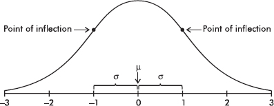
The normal distribution curve is bell-shaped and symmetric and has an infinite base. Long, flat-looking tails cover many values but only a small proportion of the area. The flat appearance of the tails is deceptive. Actually, far out in the tails, the curve drops proportionately at an ever-increasing rate. In other words, when two intervals of equal length are compared, the one closer to the center may experience a greater numerical drop, but the one further out in the tail experiences a greater drop when measured as a proportion of the height at the beginning of the interval.
The mean here is the same as the median and is located at the center. We want a unit of measurement that applies equally well to any normal distribution, and we choose a unit that arises naturally out of the curve’s shape. There is a point on each side where the slope is steepest. These two points are called points of inflection, and the distance from the mean to either point is precisely equal to one standard deviation. Thus, it is convenient to measure distances under the normal curve in terms of z-scores (recall from Topic 2 that z-scores are fractions or multiples of standard deviations from the mean).
TIP
The notation N(µ, ) stands for a normal model with mean µ and standard deviation .
Mathematically, the formula for the normal curve turns out to be y = e –z2/2, where y is the relative height above z-score. (By relative height we mean proportion of the height above the mean.) However, our interest is not so much in relative heights under the normal curve as it is in proportionate areas. The probability associated with any interval under the normal curve is equal to the proportionate area found under the curve and above the interval.
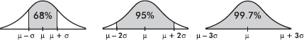
A useful property of the normal curve is that approximately 68% of the area (and thus 68% of the observations) falls within one standard deviation of the mean, approximately 95% of the area falls within two standard deviations of the mean, and approximately 99.7% of the area falls within three standard deviations of the mean.
USING TABLES OF THE NORMAL DISTRIBUTION
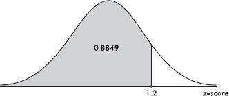
Table A in the Appendix shows areas under the normal curve. Specifically, this table shows the area to the left of a given point. It shows, for example, that to the left of a z-score of 1.2 there is 0.8849 of the area:
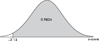
Because the total area is 1, the area to the right of a point can be calculated by calculating 1 minus the area to the left of the point. For example, the area to the right of a z-score of – 2.13 is 1 – 0.0166 = 0.9834. (Alternatively, by symmetry, we could have said that the area to the right of –2.13 is the same as that to the left of +2.13 and then read the answer directly from Table A.)
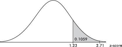
The area between two points can be found by subtraction. For example, the area between the z-scores of 1.23 and 2.71 is equal to 0.9966 – 0.8907 = 0.1059.
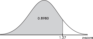
Given a probability, we can use Table A in reverse to find the appropriate z-score. For example, to find the z-score that has an area of 0.8982 to the left of it, we search for the probability closest to 0.8982 in the bulk of the table and read off the corresponding z-score. In this case we find 0.8980 with the z-score 1.27.
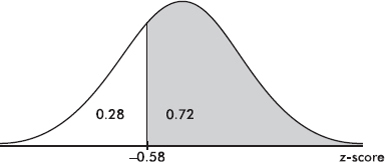
To find the z-score with an area of 0.72 to the right of it, we look for 1– 0.72 = 0.28 in the bulk of the table. The probability 0.2810 corresponds to the z-score –0.58.
USING A CALCULATOR WITH AREAS UNDER A NORMAL CURVE
On the TI-84, normalcdf(lowerbound, upperbound) gives the area (probability) between two z-scores, while invNorm(area) gives the z-score with the given area to its left. So we could have calculated above:
normalcdf(–100, 1.2) = 0.8849
normalcdf(–2.13, 100) = 0.9834
normalcdf(1.23, 2.71) = 0.1060
invNorm(.8982) = 1.271
invNorm(.28) = –0.5828
The TI-84 also has the capability of working directly with raw scores instead of z-scores. In this case, the mean and standard deviation must be given:
normalcdf(lowerbound, upperbound, mean, SD)
invNorm(area, mean, SD)
THE NORMAL DISTRIBUTION AS A MODEL FOR MEASUREMENT
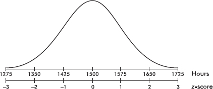
In solving a problem using the normal distribution as a model, drawing a picture of a normal curve with horizontal lines showing raw scores and z-scores is usually helpful.
 EXAMPLE 11.1
The life expectancy of a particular brand of lightbulb is normally distributed with a mean of 1500 hours and a standard deviation of 75 hours.
TIP
Don’t use the normal model if the distribution isn’t symmetric and unimodal.
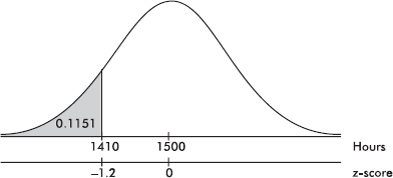
a. What is the probability that a lightbulb will last less than 1410 hours?
TIP
Draw a picture!
Answer: The z-score of 1410 is  = –1.2, and from
Table A the probability to the left of –1.2 is 0.1151. [On the TI-84, normalcdf(0, 1410, 1500, 75) = 0.1151 and normalcdf(–10, –1.2) = 0.1151.]
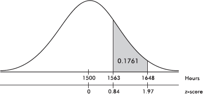
b. What is the probability that a lightbulb will last between 1563 and 1648 hours?
Answer: The z-score of 1563 is  and the z-score of 1648 is
  In Table A, 0.84 and 1.97 give probabilities of 0.7995 and 0.9756, respectively. Thus between 1563 and 1648 there is a probability of 0.9756 – 0.7995 = 0.1761. [normalcdf(1563, 1648, 1500, 75) = 0.1762 and normalcdf(.84, 1.97) = 0.1760.]
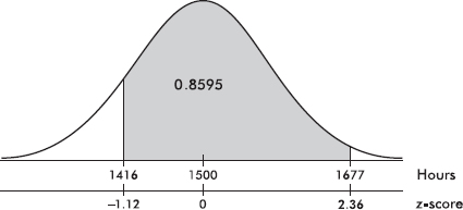
c. What is the probability that a lightbulb will last between 1416 and 1677 hours?
Answer: The z-score of 1416 is 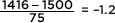 and the z-score of 1677 is
 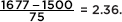 In Table A, –1.12 gives a probability of 0.1314, and 2.36 gives a probability of 0.9909. Thus between 1416 and 1677 there is a probability of 0.9909 – 0.1314 = 0.8595. [normalcdf(1416, 1677, 1500, 75) = 0.8595 and normalcdf(–1.12, 2.36) = 0.8595.]
EXAMPLE 11.2
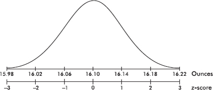
A packing machine is set to fill a cardboard box with a mean of 16.1 ounces of cereal. Suppose the amounts per box form a normal distribution with a standard deviation equal to 0.04 ounce.
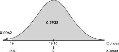
a. What percentage of the boxes will end up with at least 1 pound of cereal?
Answer: The z-score of 16 is  and –2.5 in Table A gives a probability of 0.0062. Thus the probability of having more than 1 pound in a box is 1 – 0.0062 = 0.9938 or 99.38%. [normalcdf(16, 1000, 16.10, .04) = 0.9938 and normalcdf(–2.5, 10) = 0.9938.]
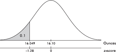
b. Ten percent of the boxes will contain less than what number of ounces?
Answer: In Table A, we note that .1 area (actually 0.1003) is found to the left of a –1.28 z-score. [On the TI-84, invNorm(.1) = –1.2816.] Converting the z-score of –1.28 into a raw score yields  ounces. [Or directly on the TI-84, invNorm(.1, 16.10, .04) = 16.049.]
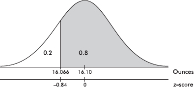
c. Eighty percent of the boxes will contain more than what number of ounces?
Answer: In Table A, we note that 1 – 0.8 = 0.2 area (actually 0.2005) is found to the left of a z-score of –0.84, and so to the right of a –0.84 z-score must be 80% of the area. [Or invNorm(.2) = 0.8416.] Converting the z-score of –0.84 into a raw score yields 16.1 – 0.84(0.04) = 16.066 ounces. [Or directly on the TI-84, invNorm(.2, 16.10, .04) = 16.066.]
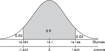
d. The middle 90% of the boxes will be between what two weights?
Answer: Ninety percent in the middle leaves five percent in each tail. In Table A, we note that .0505 area is found to the left of a z-score of –1.64, while 0.495 area is found to the left of a z-score of –1.65, and so we use the z-score of –1.645. Then 90% of the area is between z-scores of –1.645 and 1.645. [Or invNorm(.05) = –1.6449 and invNorm(.95) = 1.6449.] Converting z-scores to raw scores yields 16.1 – 1.645(0.04) = 16.034 ounces and 16.1 + 1.645(0.04) = 16.166 ounces, respectively, for the two weights between which we will find the middle 90% of the boxes. [invNorm(.05, 16.10, .04) = 16.034 and invNorm(.95, 16.10, .04) = 16.166.]
COMMONLY USED PROBABILITIES AND Z-SCORES
As can be seen from Example 11.2d, there is often an interest in the limits enclosing some specified middle percentage of the data. For future reference, the limits most frequently asked for are noted below in terms of z-scores.
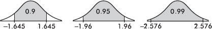
Ninety percent of the values are between z-scores of –1.645 and +1.645, 95% of the values are between z-scores of –1.96 and +1.96, and 99% of the values are between z-scores of –2.576 and +2.576.
Sometimes the interest is in values with particular percentile rankings. For example,
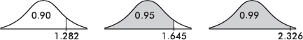
Ninety percent of the values are below a z-score of 1.282, 95% of the values are below a z-score of 1.645, and 99% of the values are below a z-score of 2.326.
There are corresponding conclusions for negative z-scores:
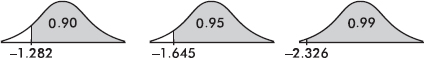
Ninety percent of the values are above a z-score of –1.282, 95% of the values are above a z-score of –1.645, and 99% of the values are above a z-score of –2.326.
It is also useful to note the percentages corresponding to values falling between integer z-scores. For example,

Note that 68.26% of the values are between z-scores of –1 and +1, 95.44% of the values are between z-scores of –2 and +2, and 99.74% of the values are between z-scores of –3 and +3.
EXAMPLE 11.3
Suppose that the average height of adult males in a particular locality is 70 inches with a standard deviation of 2.5 inches.
a. If the distribution is normal, the middle 95% of males are between what two heights?
Answer: As noted above, the critical z-scores in this case are ±1.96, and so the two limiting heights are 1.96 standard deviations from the mean. Therefore, 70 ± 1.96(2.5) = 70 ± 4.9, or from 65.1 to 74.9 inches.
b. Ninety percent of the heights are below what value?
Answer: The critical z-score is 1.282, and so the value in question is 70 + 1.282(2.5) = 73.205 inches.
c. Ninety-nine percent of the heights are above what value?
Answer: The critical z-score is –2.326, and so the value in question is 70 – 2.326(2.5) = 64.185 inches.
d. What percentage of the heights are between z-scores of ±1? Of ±2? Of ±3?
Answer: 68.26%, 95.44%, and 99.74%, respectively.
FINDING MEANS AND STANDARD DEVIATIONS
If we know that a distribution is normal, we can calculate the mean µ and the standard deviation using percentage information from the population.
EXAMPLE 11.4
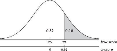
Given a normal distribution with a mean of 25, what is the standard deviation if 18% of the values are above 29?
Answer: Looking for a 0.82 probability in Table A, we note that the corresponding z-score is 0.92. Thus 29 – 25 = 4 is equal to a standard deviation of 0.92, that is, 0.92 = 4, and 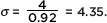
EXAMPLE 11.5
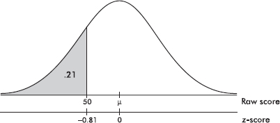
Given a normal distribution with a standard deviation of 10, what is the mean if 21% of the values are below 50?
Answer: Looking for a 0.21 probability in Table A leads us to a z-score of –0.81. Thus 50 is –0.81 standard deviation from the mean, and so µ = 50 + 0.81(10) = 58.1.
EXAMPLE 11.6
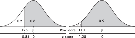
Given a normal distribution with 80% of the values above 125 and 90% of the values above 110, what are the mean and standard deviation?
Answer: Table A gives critical z-scores of –0.84 and –1.28. Thus we have 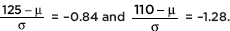 Solving the system {125 – µ = –0.84, 110 – µ = –1.28} simultaneously gives µ = 153.64 and = 34.09.
NORMAL APPROXIMATION TO THE BINOMIAL
Many practical applications of the binomial involve examples in which n is large. However, for large n, binomial probabilities can be quite tedious to calculate. Since the normal can be viewed as a limiting case of the binomial, it is natural to use the normal to approximate the binomial in appropriate situations.
TIP
When n is small, you cannot use the normal model to approximate the binomial model.
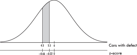
The binomial takes values only at integers, while the normal is continuous with probabilities corresponding to areas over intervals. Therefore, we establish a technique for converting from one distribution to the other. For approximation purposes we do as follows. Each binomial probability corresponds to the normal probability over a unit interval centered at the desired value. Thus, for example, to approximate the binomial probability of eight successes we determine the normal probability of being between 7.5 and 8.5.
EXAMPLE 11.7
Suppose that 15% of the cars coming out of an assembly plant have some defect. In a delivery of 40 cars what is the probability that exactly 5 cars have defects?
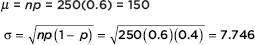
Answer: The actual answer is 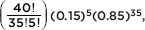 but clearly this involves a nontrivial calculation. [If one has a calculator such as the TI-84, then binompdf(40, 0.15, 5) = 0.1692.] To approximate the answer using the normal, we first calculate the mean µ and the standard deviation as follows:
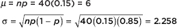
We then calculate the appropriate z-scores: 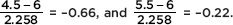
Looking up the corresponding probabilities in Table A, we obtain a final answer of 0.4129 – 0.2546 = 0.1583. (The actual answer is 0.1692.)
Even more useful are approximations relating to probabilities over intervals.
EXAMPLE 11.8
If 60% of the population support massive federal budget cuts, what is the probability that in a survey of 250 people at most 155 people support such cuts?
Answer: The actual answer is the sum of 156 binomial expressions:
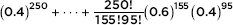
However, a good approximation can be obtained quickly and easily by using the normal. We calculate µ and :
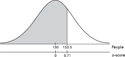
The binomial of at most 155 successes corresponds to the normal probability of ≤155.5.
The z-score of 155.5 is 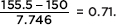 Using Table A leads us to a final answer of 0.7611. [Or binomcdf(250, .6, 155) = 0.7605.]
Is the normal a good approximation? The answer, of course, depends on the error tolerances in particular situations. A general rule of thumb is that the normal is a good approximation to the binomial whenever both np and n(1 – p) are greater than 10. (Some authors use 5 instead of 10 here.)
In the examples in this Topic we have assumed the population has a normal distribution. When you collect your own data, before you can apply the procedures developed above, you must decide whether it is reasonable to assume the data come from a normal population. In later Topics we will have to check for normality before applying certain inference procedures.
The initial check should be to draw a picture. Dotplots, stemplots, boxplots, and histograms are all useful graphical displays to show that data is unimodal and roughly symmetric.
EXAMPLE 11.9
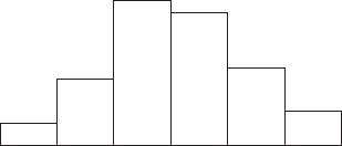
The ages at inauguration of U.S. presidents from Washington to G. W. Bush were: {57, 61, 57, 57, 58, 57, 61, 54, 68, 51, 49, 64, 50, 48, 65, 52, 56, 46, 54, 49, 51, 47, 55, 55, 54, 42, 51, 56, 55, 51, 54, 51, 60, 61, 43, 55, 56, 61, 52, 69, 64, 46, 54}. Can we conclude that the distribution is roughly normal?
Answer: Entering the 43 data points in a graphing calculator gives the following histogram:
Alternatively, we could have used a dotplot, stemplot, or boxplot:
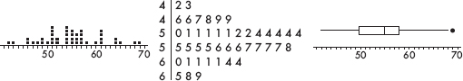
All the graphical displays indicate a distribution that is roughly unimodal and symmetric.
A more specialized graphical display to check normality is the normal probability plot. When the data distribution is roughly normal, the plot is roughly a diagonal straight line. While this plot more clearly shows deviations from normality, it is not as easy to understand as a histogram. The normal probability plot is difficult to calculate by hand; however, technology such as the TI-84 readily plots the graph. (On the TI-84, in STATPLOT the sixth choice in TYPE gives the normal probability plot.)
The normal probability plot for the data in Example 11.9 is:
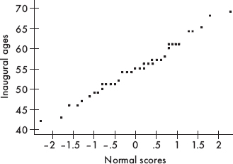
A graph this close to a diagonal straight line indicates that the data have a distribution very close to normal.
Note that alternatively, one could have plotted the data (in this case, inaugural ages) on the x-axis and the normal scores on the y-axis.
SUMMARY
 The normal distribution is one particular symmetric, unimodal distribution.
Drawing pictures of normal curves with horizontal lines showing raw scores and z-scores is usually helpful.
Areas (probabilities) under a normal curve can be found using the given table or calculator functions, such as normalcdf on TI calculators.
Critical values corresponding to given probabilities can be found using the given table or calculator functions, such as invNorm on TI calculators.
The normal probability plot is very useful in gauging whether a given distribution of data is approximately normal: If the plot is nearly straight, the data is nearly normal.
QUESTIONS ON TOPIC ELEVEN: THE NORMAL DISTRIBUTION
Multiple-Choice Questions
Directions: The questions or incomplete statements that follow are each followed by five suggested answers or completions. Choose the response that best answers the question or completes the statement.
1. Which of the following is a true statement?
(A) The area under a normal curve is always equal to 1, no matter what the mean and standard deviation are.
(B) All bell-shaped curves are normal distributions for some choice of µ and .
(C) The smaller the standard deviation of a normal curve, the lower and more spread out the graph.
(D) Depending upon the value of the standard deviation, normal curves with different means may be centered around the same number.
(E) Depending upon the value of the standard deviation, the mean and median of a particular normal distribution may be different.
2. Which of the following is a true statement?
(A) The area under the standard normal curve between 0 and 2 is twice the area between 0 and 1.
(B) The area under the standard normal curve between 0 and 2 is half the area between –2 and 2.
(C) For the standard normal curve, the interquartile range is approximately 3.
(D) For the standard normal curve, the range is 6.
(E) For the standard normal curve, the area to the left of 0.1 is the same as the area to the right of 0.9.
3. Populations P1 and P2 are normally distributed and have identical means. However, the standard deviation of P1 is twice the standard deviation of P2. What can be said about the percentage of observations falling within two standard deviations of the mean for each population?
(A) The percentage for P1 is twice the percentage for P2.
(B) The percentage for P1 is greater, but not twice as great, as the percentage for P2.
(C) The percentage for P2 is twice the percentage for P1.
(D) The percentage for P2 is greater, but not twice as great, as the percentage for P1.
(E) The percentages are identical.
4. Consider the following two normal curves:
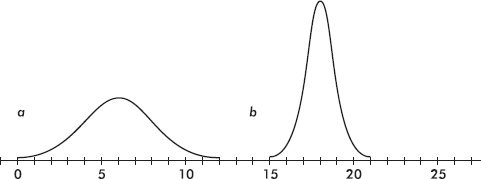
Which has the larger mean and which has the larger standard deviation?
(A) Larger mean, a; larger standard deviation, a
(B) Larger mean, a; larger standard deviation, b
(C) Larger mean, b; larger standard deviation, a
(D) Larger mean, b; larger standard deviation, b
(E) Larger mean, b; same standard deviation
In Questions 5–15, assume the given distributions are normal.
5. A trucking firm determines that its fleet of trucks averages a mean of 12.4 miles per gallon with a standard deviation of 1.2 miles per gallon on cross-country hauls. What is the probability that one of the trucks averages fewer than 10 miles per gallon?
(A) 0.0082
(B) 0.0228
(C) 0.4772
(D) 0.5228
(E) 0.9772
6. A factory dumps an average of 2.43 tons of pollutants into a river every week. If the standard deviation is 0.88 tons, what is the probability that in a week more than 3 tons are dumped?
(A) 0.2578
(B) 0.2843
(C) 0.6500
(D) 0.7157
(E) 0.7422
7. An electronic product takes an average of 3.4 hours to move through an assembly line. If the standard deviation is 0.5 hour, what is the probability that an item will take between 3 and 4 hours?
(A) 0.2119
(B) 0.2295
(C) 0.3270
(D) 0.3811
(E) 0.6730
8. The mean score on a college placement exam is 500 with a standard deviation of 100. Ninety-five percent of the test takers score above what?
(A) 260
(B) 336
(C) 405
(D) 414
(E) 664
9. The average noise level in a restaurant is 30 decibels with a standard deviation of 4 decibels. Ninety-nine percent of the time it is below what value?
(A) 20.7
(B) 32.0
(C) 33.4
(D) 37.8
(E) 39.3
10. The mean income per household in a certain state is $9500 with a standard deviation of $1750. The middle 95% of incomes are between what two values?
(A) $5422 and $13,578
(B) $6070 and $12,930
(C) $6621 and $12,379
(D) $7260 and $11,740
(E) $8049 and $10,951
11. One company produces movie trailers with mean 150 seconds and standard deviation 40 seconds, while a second company produces trailers with mean 120 seconds and standard deviation 30 seconds. What is the probability that two randomly selected trailers, one produced by each company, will combine to less than three minutes?
(A) 0.000
(B) 0.036
(C) 0.099
(D) 0.180
(E) 0.405
12. Jay Olshansky from the University of Chicago was quoted in Chance News as arguing that for the average life expectancy to reach 100, 18% of people would have to live to 120. What standard deviation is he assuming for this statement to make sense?
(A) 21.7
(B) 24.4
(C) 25.2
(D) 35.0
(E) 111.1
13. Cucumbers grown on a certain farm have weights with a standard deviation of 2 ounces. What is the mean weight if 85% of the cucumbers weigh less than 16 ounces?
(A) 13.92
(B) 14.30
(C) 14.40
(D) 14.88
(E) 15.70
14. If 75% of all families spend more than $75 weekly for food, while 15% spend more than $150, what is the mean weekly expenditure and what is the standard deviation?
(A) µ = 83.33, = 12.44
(B) µ = 56.26, = 11.85
(C) µ = 118.52, = 56.26
(D) µ = 104.39, = 43.86
(E) µ = 139.45, = 83.33
15. A coffee machine can be adjusted to deliver any fixed number of ounces of coffee. If the machine has a standard deviation in delivery equal to 0.4 ounce, what should be the mean setting so that an 8-ounce cup will overflow only 0.5% of the time?
(A) 6.97 ounces
(B) 7.22 ounces
(C) 7.34 ounces
(D) 7.80 ounces
(E) 9.03 ounces
16. Assume that a baseball team has an average pitcher, that is, one whose probability of winning any decision is 0.5. If this pitcher has 30 decisions in a season, what is the probability that he will win at least 20 games?
(A) 0.0505
(B) 0.2514
(C) 0.2743
(D) 0.3333
(E) 0.4300
17. Given that 10% of the nails made using a certain manufacturing process have a length less than 2.48 inches, while 5% have a length greater than 2.54 inches, what are the mean and standard deviation of the lengths of the nails? Assume that the lengths have a normal distribution.
(A) µ = 2.506, = 0.0205
(B) µ = 2.506, = 0.0410
(C) µ = 2.516, = 0.0825
(D) µ = 2.516, = 0.1653
(E) The mean and standard deviation cannot be computed from the information given.
Free-Response Questions
Directions: You must show all work and indicate the methods you use. You will be graded on the correctness of your methods and on the accuracy of your final answers.
TWO OPEN-ENDED QUESTIONS
1. The time it takes Steve to walk to school follows a normal distribution with mean 30 minutes and standard deviation 5 minutes, while the time it takes Jan to walk to school follows a normal distribution with mean 25 minutes and standard deviation 4 minutes. Assume their walking times are independent of each other.
(a) If they leave at the same time, what is the probability that Steve arrives before Jan?
(b) How much earlier than Jan should Steve leave so that he has a 90% chance of arriving before Jan?
2. (a) Two components are in series so the failure of either will cause the system to fail. The time to failure for a new component is normally distributed with a mean of 3000 hours and a standard deviation of 400 hours. One of the components has already run for 2500 hours, while the other has run for 2800 hours. Assuming component failures are independent, what is the probability the system survives for 10 more days (240 hours)?
(b) If the components are put in parallel, the system will fail only if both components fail. If the two components in (a) are put in parallel, what is the probability that the system survives for 10 more days?
TWO INVESTIGATIVE TASKS
1. When Michael Jordan came up to try for a sixth free throw after having made five straight free throws, the announcer commented that the law of averages would be working against Jordan.
(a) What did the announcer mean? Was this a correct interpretation of probability? Explain.
(b) Jordan makes 90% of his free throws. What is the probability that he will make six straight free throws? That he will make five straight free throws and then miss the next? That he will make the next free throw given that he has made the last five in a row?
(c) How could you set up a simulation using a random number table to analyze the situation the announcer was commenting on?
(d) If Jordan shoots six times from the free throw line, what are the mean and standard deviation for the number of shots he is expected to make?
(e) If Jordan makes only 35 out of 40 free throw tries during the playoffs, is this sufficient evidence that the probability of his making a free throw is really below .90? Explain.
2. Many people have lactose intolerance leading to cramps and diarrhea when they eat dairy products. Substantial relief can be obtained by taking dietary supplements of lactase, an enzyme. One product consists of caplets containing a mean of 9000 FCC lactase units with a standard deviation of 590 units and a normal distribution of lactase units. People with severe lactose intolerance may need to take two such tablets whenever they eat dairy products. Tablets with under 8500 FCC lactase units can produce noticeably less relief.
(a) Determine the probability that a caplet has less than 8500 FCC lactase units. Round off to the nearest tenth.
(b) Using the random number table below, run five simulations for the number of tablets a lab technician samples before finding two with less than 8500 units each.
84177 06757 17613 15582 51506 81435 41050 92031 06449 05059
59884 31180 53115 84469 94868 57967 05811 84514 75011 13006
63395 55041 15866 06589 13119 71020 85940 91932 06488 74987
54355 52704 90359 02649 47496 71567 94268 08844 26294 64759
08989 57024 97284 00637 89283 03514 59195 07635 03309 72605
29357 23737 67881 03668 33876 35841 52869 23114 15864 38942
(c) The results of two 100-trial simulations, one looking for two tablets each less than 8500 units and one looking for two tablets each greater than 9000 units, are shown below. Which distribution is which? Explain your answer.
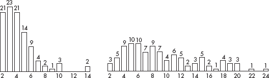
(d) Using the correct barplot above, estimate the expected number of caplets a laboratory will sample before finding two with less than 8500 units each.