SAMPLE PROPORTION
SAMPLE MEAN
CENTRAL LIMIT THEOREM
DIFFERENCE BETWEEN TWO INDEPENDENT SAMPLE PROPORTIONS
DIFFERENCE BETWEEN TWO INDEPENDENT SAMPLE MEANS
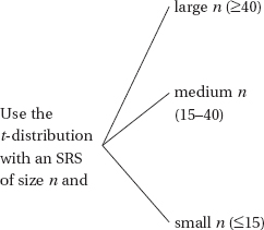
THE t-DISTRIBUTION
THE CHI-SQUARE DISTRIBUTION
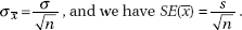
THE STANDARD ERROR
BIAS AND ACCURACY
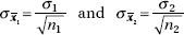
The population is the complete set of items of interest. A sample is a part of a population used to represent the population. The population mean µ and population standard deviation  are examples of population parameters. The sample mean x and the sample standard deviation s are examples of statistics. Statistics are used to make inferences about population parameters. While a population parameter is a fixed quantity, statistics vary depending on the particular sample chosen. The probability distribution showing how a statistic varies is called a sampling distribution. The sampling distribution is unbiased if its mean is equal to the associated population parameter.
IMPORTANT
A sampling distribution is not the same thing as the distribution of a sample.
We want to know some important truth about a population, but in practical terms this truth is unknowable. What’s the average adult human body weight? What proportion of people have high cholesterol? What we can do is carefully collect data from as large and representative a group of individuals as possible and then use this information to estimate the value of the population parameter. How close are we to the truth? We know that different samples would give different estimates, and so sampling error is unavoidable. What is wonderful, and what we will learn in this Topic, is that we can quantify this sampling error! We can make statements like “the average weight must almost surely be within 5 pounds of 176 pounds” or “the proportion of people with high cholesterol must almost surely be within ±3% of 37%.”
SAMPLING DISTRIBUTION OF A SAMPLE PROPORTION
Whereas the mean is basically a quantitative measurement, the proportion represents essentially a qualitative approach. The interest is simply in the presence or absence of some attribute. We count the number of yes responses and form a proportion. For example, what proportion of drivers wear seat belts? What proportion of SCUD missiles can be intercepted? What proportion of new stereo sets have a certain defect?
This separation of the population into “haves” and “have-nots” suggests that we can make use of our earlier work on binomial distributions. We also keep in mind that, when n (trials, or in this case sample size) is large enough, the binomial can be approximated by the normal.
In this topic we are interested in estimating a population proportion p by considering a single sample proportion  . This sample proportion is just one of a whole universe of sample proportions, and to judge its significance we must know how sample proportions vary. Consider the set of proportions from all possible samples of a specified size n. It seems reasonable that these proportions will cluster around the population proportion (the sample proportion is an unbiased statistic of the population proportion) and that the larger the chosen sample size, the tighter the clustering.
How do we calculate the mean and standard deviation of the set of population proportions? Suppose the sample size is n and the actual population proportion is p. From our work on binomial distributions, we remember that the mean and standard deviation for the number of successes in a given sample are pn and  respectively, and for large n the complete distribution begins to look “normal.”
Here, however, we are interested in the proportion rather than in the number of successes. From Topic Two we remember that when we multiply or divide every element by a constant, we multiply or divide both the mean and the standard deviation by the same constant. In this case, to change number of successes to proportion of successes, we divide by n:
Furthermore, if each element in an approximately normal distribution is divided by the same constant, it is reasonable that the result will still be an approximately normal distribution.
Thus the principle forming the basis of the following discussion is
Start with a population with a given proportion p. Take all samples of size n. Compute the proportion in each of these samples. Then
1. the set of all sample proportions is approximately normally distributed (often stated: the distribution of sample proportions is approximately normal).
2. the mean µ of the set of sample proportions equals p, the population proportion.
3. the standard deviation of the set of sample proportions is approximately equal to 
Alternatively, we say that the sampling distribution of is approximately normal with mean p and standard deviation 
Since we are using the normal approximation to the binomial, both np and n(1 – p) should be at least 10. Furthermore, in making calculations and drawing conclusions from a specific sample, it is important that the sample be a simple random sample.
Finally, because sampling is usually done without replacement, the sample cannot be too large; the sample size n should be no larger than 10% of the population. (We’re actually worried about independence, but randomly selecting a relatively small sample allows us to assume independence. Of course, it’s always better to have larger samples—it’s just that if the sample is large relative to the population, then the proper inference techniques are different from those taught in introductory statistics classes.)
TIP
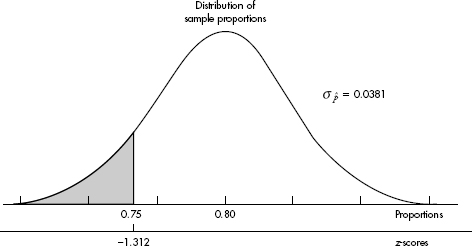
It is sufficient to write: Normal with µ = 0.80 and = 0.0381; P( < 0.75) = 0.0947.
 EXAMPLE 12.1
It is estimated that 80% of people with high math anxiety experience brain activity similar to that experienced under physical pain when anticipating doing a math problem. In a simple random sample of 110 people with high math anxiety, what is the probability that less than 75% experience the physical pain brain activity?
Answer: The sample is given to be random, both np = (110)(0.80) = 88  10 and n(1 – p) = (110)(0.20) = 22 10, and our sample is clearly less than 10% of all people with math anxiety. So the sampling distribution of is approximately normal with mean 0.80 and standard deviation
 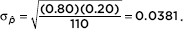 With a z-score of
 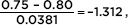 the probability that the sample proportion is less than 0.75 is normalcdf(–1000,–1.312) = 0.0948.
[Or normalcdf(–1000, .75, .80, .0381) = 0.0947.]
SAMPLING DISTRIBUTION OF A SAMPLE MEAN
Suppose we are interested in estimating the mean µ of a population. For our estimate we could simply randomly pick a single element of the population, but then we would have little confidence in our answer. Suppose instead that we pick 100 elements and calculate their average. It is intuitively clear that the resulting sample mean has a greater chance of being closer to the mean of the whole population than the value for any individual member of the population does.
When we pick a sample and measure its mean x, we are finding exactly one sample mean out of a whole universe of sample means. To judge the significance of a single sample mean, we must know how sample means vary. Consider the set of means from all possible samples of a specified size. It is both apparent and reasonable that the sample means are clustered around the mean of the whole population; furthermore, these sample means have a tighter clustering than the elements of the original population. In fact, we might guess that the larger the chosen sample size, the tighter the clustering.
How do we calculate the standard deviation  of the set of sample means? Suppose the variance of the population is 2 and we are interested in samples of size n. Sample means are obtained by first summing together n elements and then dividing by n. A set of sums has a variance equal to the sum of the variances associated with the original sets. In our case, 2sums = 2 + · · · + 2 = n2. When each element of a set is divided by some constant, the new variance is the old one divided by the square of the constant. Since the sample means are obtained by dividing the sums by n, the variance of the sample means is obtained by dividing the variance of the sums by n2. Thus if symbolizes the standard deviation of the sample means, we find that
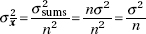
In terms of standard deviations, we have 
We have shown the following:
Start with a population with a given mean μ and standard deviation . Compute the mean of all samples of size n. Then the mean of the set of sample means will equal μ, the mean of the population, and the standard deviation x of the set of sample means will equal  that is, the standard deviation of the whole population divided by the square root of the sample size.
Note that the variance of the set of sample means varies directly as the variance of the original population and inversely as the size of the samples, while the standard deviation of the set of sample means varies directly as the standard deviation of the original population and inversely as the square root of the size of the samples.
EXAMPLE 12.2
Emergency room visits after drinking energy drinks is skyrocketing. One particular energy drink has an average of 200 mg of caffeine with a standard deviation of 10 mg. A store sells boxes of six bottles each. What is the mean and standard deviation of the average milligrams of caffeine consumers should expect from the six bottles in each box?
Answer: We have samples of size 6. The mean of these sample means will equal the population mean of 200 mg. The standard deviation of these sample means will
equal 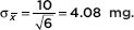
Note that while giving the mean and standard deviation of the set of sample means, we did not describe the shape of the distribution. If we are also given that the original population is normal, then we can conclude that the set of sample means has a normal distribution.
EXAMPLE 12.3
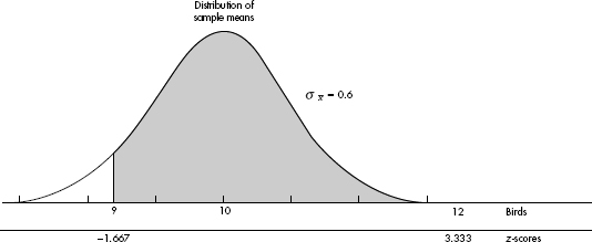
It is estimated that cats, who live in the wild or as indoor pets allowed to roam outdoors, kill an average of 10 birds a year. Assuming a normal distribution with a standard deviation of 3 birds, what is the probability an SRS of 25 cats will kill an average of between 9 and 12 birds in a year?
Answer: The sampling distribution of the sample means is approximately normal (because the original population is normal) with mean µx = 10 and standard deviation  The z-scores of 9 and 12 are
 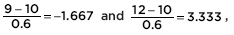 and the probability of a sample mean between 9 and 12 is normalcdf(-1.667,3.333) = 0.952. [Or normalcdf(9,12,10,0.6) = 0.952.]
We assumed above that the original population had a normal distribution. Unfortunately, few populations are normal, let alone exactly normal. However, it can be shown mathematically that no matter how the original population is distributed, if n is large enough, then the set of sample means is approximately normally distributed. For example, there is no reason to suppose that the amounts of money that different people spend in grocery stores are normally distributed. However, if each day we survey 30 people leaving a store and determine the average grocery bill, these daily averages will have a nearly normal distribution.
The following principle forms the basis of much of what we discuss in this topic and in those following. It is a simplified statement of the central limit theorem of statistics.
Start with a population with a given mean μ, a standard deviation , and any shape distribution whatsoever. Pick n sufficiently large (at least 30) and take all samples of size n. Compute the mean of each of these samples. Then
1. the set of all sample means is approximately normally distributed (often stated: the distribution of sample means is approximately normal).
2. the mean of the set of sample means equals μ, the mean of the population.
3. the standard deviation x of the set of sample means is equal to  that is, equal to the standard deviation of the whole population divided by the square root of the sample size.
Alternatively, we say that the sampling distribution of x is approximately normal with mean μ and standard deviation 
While we mention n 30 as a rough rule of thumb, n 40 is often used, and n should be chosen even larger if more accuracy is required or if the original population is far from normal. As with proportions, we have the assumptions of a simple random sample and of sample size n no larger than 10% of the population.
EXAMPLE 12.4
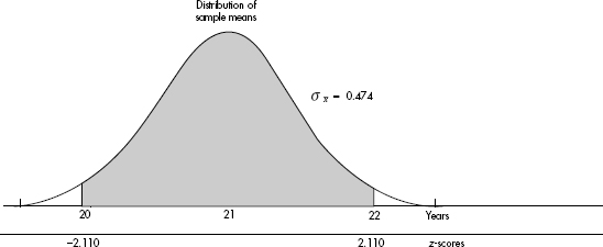
The naked mole rat, a hairless East African rodent that lives underground, has a life expectancy of 21 years with a standard deviation of 3 years. In a random sample of 40 such rats, what is the probability that the mean life expectancy is between 20 and 22 years?
Answer: We have a random sample that is less than 10% of the naked mole rat population. With a sample size of 40, the central limit theorem applies, and the sampling distribution of x is approximately normal with mean µx = 21 and standard deviation  The z-scores of 20 and 22 are
  and
and  the probability of sample mean between 20 and 22 is normalcdf(–2.110,2.110) = 0.965. [Or normalcdf(20,22,21,0.474)= 0.965.]
EXAMPLE 12.5
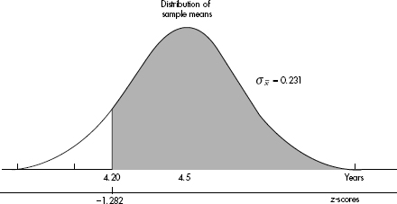
Being bilingual appears to slow the onset of dementia by an average of 4.5 years with a standard deviation of 2 years. In a random sample of 75 bilingual people with dementia, the probability is 0.90 that the average delay in the onset of their dementia was at least how many years?
Answer: We have a random sample that is less than 10% of the total bilingual dementia population. With a sample size of 75, the central limit theorem applies, and the sampling distribution of x is approximately normal with mean µx = 4.5 and standard deviation 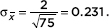 The critical z-score is invNorm(0.10)= –1.282 with a corresponding raw score of 4.5 – 1.282(0.231) = 4.20 years. [Or invNorm(.10,4.5,.231)= 4.20.]
Don’t be confused by the several different distributions being discussed! First, there’s the distribution of the original population, which may be uniform, bell-shaped, strongly skewed—anything at all. Second, there’s the distribution of the data in the sample, and the larger the sample size, the more this will look like the population distribution. Third, there’s the distribution of the means of many samples of a given size, and the amazing fact is that this sampling distribution can be described by a normal model, regardless of the shape of the original population.
SAMPLING DISTRIBUTION OF A DIFFERENCE BETWEEN TWO INDEPENDENT SAMPLE PROPORTIONS
Numerous important and interesting applications of statistics involve the comparison of two population proportions. For example, is the proportion of satisfied purchasers of American automobiles greater than that of buyers of Japanese cars? How does the percentage of surgeons recommending a new cancer treatment compare with the corresponding percentage of oncologists? What can be said about the difference between the proportion of single parents on welfare and the proportion of two-parent families on welfare?
Our procedure involves comparing two sample proportions. When is a difference between two such sample proportions significant? Note that we are dealing with one difference from the set of all possible differences obtained by subtracting sample proportions of one population from sample proportions of a second population. To judge the significance of one particular difference, we must first determine how the differences vary among themselves. Remember that the variance of a set of differences is equal to the sum of the variances of the individual sets; that is,

Now if
then

Then we have the following about the sampling distribution of 1 – 2:
Start with two populations with given proportions p1 and p2. Take all samples of sizes n1 and n2, respectively. Compute the difference 1 – 2 of the two proportions in each pair of samples. Then
1. the set of all differences of sample proportions is approximately normally distributed (alternatively stated: the distribution of differences of sample proportions is approximately normal).
2. the mean of the set of differences of sample proportions equals p1 – p2, the difference of population proportions.
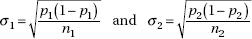
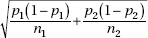
3. the standard deviation d of the set of differences of sample proportions is approximately equal to
Since we are using the normal approximation to the binomial, n1p1, n1(1 – p1), n2p2, and n2(1 – p2) should all be at least 10. Furthermore, in making calculations and drawing conclusions from specific samples, it is important both that the samples be simple random samples and that they be taken independently of each other. Finally, each sample cannot be too large; the sample sizes should be no larger than 10% of the populations.
EXAMPLE 12.6
In a study of how environment affects our eating habits, scientists revamped one of two close-to-each-other fast-food restaurants with table cloths, candlelight, and soft music. They then noted that at the revamped restaurant customers ate slower and 25% left at least 100 calories of food on their plates. At the unrevamped garish restaurant, customers tended to wolf down their food, and only 19% left at least 100 calories of food on their plates. In a random sample of 110 customers at the revamped restaurant and an independent random sample of 120 customers at the unrevamped restaurant, what is the probability that the difference in the percentages of customers in the revamped setting and unrevamped setting is more than 10% (where the difference is the revamped restaurant percent minus the unrevamped restaurant percent)?
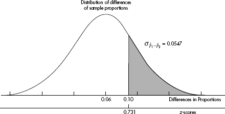
Answer: We have independent random samples, each less than 10% of all fast-food customers, and we note that n1p1 = 110(0.25) = 27.5, n1(1 – p1) = 110(0.75) = 82.5, n2p2 = 120(0.19) = 22.8, and n2(1 – p2) = 120(0.81) = 97.2 are all 10. Thus, the sampling distribution of 1 – 2 is roughly normal with mean µ1 – 2 = 0.25 – 0.19 = 0.06 and standard deviation 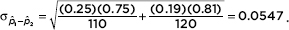 The z-score of 0.10 is
 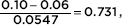 and normalcdf (.731,1000)= 0.232.
[Or normalcdf(0.10,1.0,0.06,0.0547)= 0.232.]
SAMPLING DISTRIBUTION OF A DIFFERENCE BETWEEN TWO INDEPENDENT SAMPLE MEANS
Many real-life applications of statistics involve comparisons of two population means. For example, is the average weight of laboratory rabbits receiving a special diet greater than that of rabbits on a standard diet? Which of two accounting firms pays a higher mean starting salary? Is the life expectancy of a coal miner less than that of a school teacher?
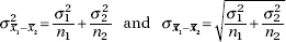
First we consider how to compare the means of samples, one from each population. When is a difference between two such sample means significant? The answer is more apparent when we realize that what we are looking at is one difference from a set of differences. That is, there is the set of all possible differences obtained by subtracting sample means from one set from sample means from a second set. To judge the significance of one particular difference we must first determine how the differences vary among themselves. The necessary key is the fact that the variance of a set of differences is equal to the sum of the variances of the individual sets. Thus,

Now if
then
Then we have the following about the sampling distribution of x1 – x2:
Start with two normal populations with means μ1 and μ2 and standard deviations 1 and 2. Take all samples of sizes n1 and n2, respectively. Compute the difference x1 – x2 of the two means in each pair of these samples. Then
1. the set of all differences of sample means is approximately normally distributed (alternatively stated: the distribution of differences of sample means is approximately normal).
2. the mean of the set of differences of sample means equals μ1 – μ2, the difference of population means.
3. the standard deviation x1 – x2 of the set of differences of sample means is approximately equal to 
The more either population varies from normal, the greater should be the corresponding sample size. We also have the assumptions of independent simple random samples, and of sample sizes no larger than 10% of the populations.
EXAMPLE 12.7
It is estimated that 40-year-old men contribute an average of 65 genetic mutations to their new children, whereas 20-year-old men contribute an average of only 25. Assuming standard deviations of 15 and 5 mutations respectively for the 40- and 20 year olds, what is the probability that the mean number of mutations in a random sample of thirty-five 40-year-old new fathers is between 35 and 45 more than the mean number in a random sample of forty 20-year-old new fathers?
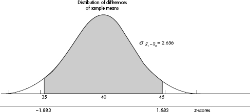
Answer: We have independent random samples, each less than 10% of their age groups, and both sample sizes are over 30, so the sampling distribution of x1 – x2 is roughly normal with mean µx–x = 65 – 25 = 40 and standard deviation 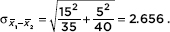 The z-scores of 35 and 45 are
 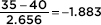 and
and 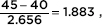 and normalcdf(-1.883,1.883)= 0.940.
[Or normalcdf(35,45,40,2.656= 0.940.]
EXAMPLE 12.8
The average number of missed school days for students going to public schools is 8.5 with a standard deviation of 4.1, while students going to private schools miss an average of 5.3 with a standard deviation of 2.9. In an SRS of 200 public school students and an SRS of 150 private school students, with a probability of 0.95 the difference in average missed days (public average minus private average) is above what number?
Answer: We have large (n1 = 200 and n2 = 150) SRSs that are still smaller than 10% of all public and private school students. The mean of the differences is 8.5 – 5.3 = 3.2, while the standard deviation is 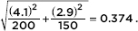 An area of 0.95 to the right corresponds to a z-score of –1.645. The difference in days is 3.2 – 1.645(0.374) = 2.6. Thus there is a 0.95 probability that the difference in average missed days between public and private school samples is over 2.6 days. [invNorm(.05, 3.2, .374) = 2.585.]
When the population standard deviation σ is unknown, we use the sample standard deviation s as an estimate for σ. But then  does not follow a normal distribution. If, however, the original population is normally distributed, there is a distribution that can be used when working with the
  ratios. This Student t-distribution was introduced in 1908 by W. S. Gosset, a British mathematician employed by the Guiness Breweries. (When we are working with small samples from a population that is not nearly normal, we must use very different “nonparametric” techniques not discussed in this review book.)
Thus, for a sample from a normally distributed population, we work with the variable

with a resulting t-distribution that is bell-shaped and symmetric, but lower at the mean, higher at the tails, and so more spread out than the normal distribution.
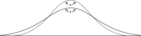
Like the binomial distribution, the t-distribution is different for different values of n. In the tables these distinct t-distributions are associated with the values for degrees of freedom (df). For this discussion the df value is equal to the sample size minus 1. The smaller the df value, the larger the dispersion in the distribution. The larger the df value, that is, the larger the sample size, the closer the distribution to the normal distribution.
Since there is a separate t-distribution for each df value, fairly complete tables would involve many pages; therefore, in Table B of the Appendix we list areas and t-values for only the more commonly used percentages or probabilities. The last row of Table B is the normal distribution, which is a special case of the t-distribution taken when n is infinite. For practical purposes, the two distributions are very close for any n 30 (some use n 40). However, when more accuracy is required, the Student t-distribution can be used for much larger values of n, and the calculations are easy with technology.
Note that, whereas Table A gives areas under the normal curve to the left of given z-values, Table B gives areas to the right of given positive t-values. For example, suppose the sample size is 20, and so df = 20 – 1 = 19. Then a probability of 0.05 in the tail corresponds with a t-value of 1.729, while 0.01 in the tail corresponds to t = 2.539.
Thus the t-distribution is the proper choice whenever the population standard deviation is unknown. In the real world is almost always unknown, and so we should almost always use the t-distribution. In the past this was difficult because extensive tables were necessary for the various t-distributions. However, with calculators such as the TI-84, this problem has diminished. It is no longer necessary to assume that the t-distribution is close enough to the z-distribution whenever n is greater than the arbitrary number 30.
The issue of sample size is refined even further by some statisticians:
|
Unnecessary to make any assumptions about parent population. |
For  to have a t-distribution, we actually need that the sampling distribution of x is normal. This follows either if the original population has a normal distribution or if the sample size is large enough (from the central limit theorem).
There is a family of sampling distribution models, called the chi-square models, which we will use for testing (not confidence intervals). The chi-square distribution has a parameter called degrees of freedom (df). For small df the distribution is skewed to the right; however, for large df it becomes more symmetric and bell-shaped (as does the t-distribution). For one or two degrees of freedom the peak occurs at 0, while for three or more degrees of freedom the peak is at df – 2.
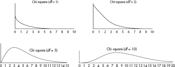
The chi-square distribution, like the t-distribution, has a separate curve for each df value; therefore, in Table C of the Appendix we list critical chi-square values for only the more commonly used tail probabilities. The chi-square distribution has numerous applications, two of the best known of which are goodness of fit of an observed distribution to a theoretical one, and independence of two criteria of classification of qualitative data. While we will be using chi-square for categorical data, the chi-square distribution as seen above is a continuous distribution, and applying it to counting data is just an approximation.
TIP
Also of note are that the mean = df, and the variance = 2df.
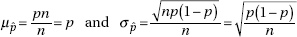
With proportions and means we typically do not know population parameters. So in calculating standard deviations of the sampling models, we actually estimate using sample statistics. In this case, we use the term standard error. That is, for proportions,
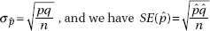
Similarly, for means,
Understand that a sampling distribution is a theoretical thing that never happens in real data analysis. When all we have is an estimate, know it is just that, only an estimate. Of course it’s wrong, but it’s the best we’ve got. This leads to a discussion of bias and accuracy.
In Topic 7 we discussed bias in the context of surveys as a tendency to favor the selection of certain members of a population. In the context of sampling distributions, bias means that the sampling distribution is not centered on the population parameter. The sampling distributions of proportions and means are unbiased, that is, for a given sample size, the set of all sample proportions is centered on the population proportion, and the set of all sample means is centered on the population mean.
The other important, quantifiable judgement of how good an estimate is is accuracy, or how narrow the sampling distribution is. For both proportions and means, this is inversely proportional to  the square root of the sample size.
SUMMARY
 Provided that the sample size n is large enough, the sampling distribution of sample proportions is approximately normal with mean p and standard deviation
  (where p is the population proportion).
Provided that the sample size n is large enough, the sampling distribution of sample means is approximately normal with mean µ and standard deviation  (where µ and are the population mean and standard deviation).
When the population standard deviation σ is unknown (which is almost always the case), and provided that the original population is normally distributed or the sample size n is large enough, the sampling distribution of sample means follows a t-distribution with mean µ and standard deviation  (where µ is the population mean and s is the sample standard deviation).
QUESTIONS ON TOPIC TWELVE: SAMPLING DISTRIBUTIONS
Multiple-Choice Questions
Directions: The questions or incomplete statements that follow are each followed by five suggested answers or completions. Choose the response that best answers the question or completes the statement.
1. Which of the following is a true statement?
(A) The larger the sample, the larger the spread in the sampling distribution.
(B) Bias has to do with the spread of a sampling distribution.
(C) Provided that the population size is significantly greater than the sample size, the spread of the sampling distribution does not depend on the population size.
(D) Sample parameters are used to make inferences about population statistics.
(E) Statistics from smaller samples have less variability.
2. Which of the following is an incorrect statement?
(A) The sampling distribution of x has mean equal to the population mean µ even if the population is not normally distributed.
(B) The sampling distribution of x has standard deviation  even if the population is not normally distributed.
(C) The sampling distribution of x is normal if the population has a normal distribution.
(D) When n is large, the sampling distribution of x is approximately normal even if the population is not normally distributed.
(E) The larger the value of the sample size n, the closer the standard deviation of the sampling distribution of x is to the standard deviation of the population.
3. Which of the following is a true statement?
(A) The sampling distribution of has a mean equal to the population proportion p.
(B) The sampling distribution of has a standard deviation equal to 
(C) The sampling distribution of has a standard deviation that becomes larger as the sample size becomes larger.
(D) The sampling distribution of is considered close to normal provided that n 30.
(E) The sampling distribution of is always close to normal.
4. In a school of 2500 students, the students in an AP Statistics class are planning a random survey of 100 students to estimate the proportion who would rather drop lacrosse rather than band during this time of severe budget cuts. Their teacher suggests instead to survey 200 students in order to
(A) reduce bias.
(B) reduce variability.
(C) increase bias.
(D) increase variability.
(E) make possible stratification between lacrosse and band.
5. The ages of people who died last year in the United States is skewed left. What happens to the sampling distribution of sample means as the sample size goes from n = 50 to n = 200?
(A) The mean gets closer to the population mean, the standard deviation stays the same, and the shape becomes more skewed left.
(B) The mean gets closer to the population mean, the standard deviation becomes smaller, and the shape becomes more skewed left.
(C) The mean gets closer to the population mean, the standard deviation stays the same, and the shape becomes closer to normal.
(D) The mean gets closer to the population mean, the standard deviation becomes smaller, and the shape becomes closer to normal.
(E) The mean stays the same, the standard deviation becomes smaller, and the shape becomes closer to normal.
6. Which of the following is the best reason that the sample maximum is not used as an estimator for the population maximum?
(A) The sample maximum is biased.
(B) The sampling distribution of the sample maximum is not binomial.
(C) The sampling distribution of the sample maximum is not normal.
(D) The sampling distribution of the sample maximum has too large a standard deviation.
(E) The sample mean plus three sample standard deviations gives a much superior estimate for the population maximum.
7. Which of the following are unbiased estimators for the corresponding population parameters?
I. Sample means
II. Sample proportions
III. Difference of sample means
IV. Difference of sample proportions
(A) None are unbiased.
(B) I and II
(C) I and III
(D) III and IV
(E) All are unbiased.
8. Thirty-four percent of Americans say that math is the most important subject in school. In a random sample of 400 Americans, what is the probability that between 30% and 35% will say that math is the most important subject?
(A) 0.291
(B) 0.337
(C) 0.382
(D) 0.618
(E) 0.709
9. Researchers found that in the aftermath of the 2011 Fukushima nuclear disaster, 12% of the pale grass blue butterfly larvae developed mutations as adults. What is the probability that in a random sample of 300 of these butterfly larvae, more than 15 developed mutations as adults?
(A) 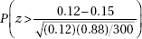
(B) 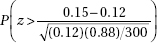
(C) 
(D) 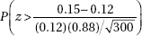
(E) 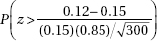
10. Suppose using accelerometers in helmets, researchers determine that boys playing high school football absorb an average of 355 hits to the head with a standard deviation of 80 hits during a season (including both practices and games). What is the probability on a randomly selected team of 48 players that the average number of head hits per player is between 340 and 360?
(A) 0.236
(B) 0.429
(C) 0.571
(D) 0.614
(E) 0.764
11. It is estimated that school CO2 levels average 1200 ppm with a standard deviation of 300 ppm. In a random sample of 30 schools, what is the probability that the mean CO2 level is more than 1000, a level at which some researchers feel will cause a drop in academic performance?
(A) 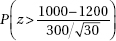
(B) 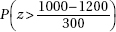
(C) 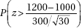
(D) 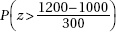
(E) 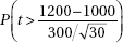
12. Binge drinking is a serious problem, killing more than 1700 college students per year. Suppose the incidence of binge drinking is 43% and 37%, respectively, at two large universities. In a random sample of 75 students at the first school and 80 students at the second, what is the probability that the difference (first minus second) between the percentages of binge drinkers is between 5% and 10%?
(A) 0.176
(B) 0.245
(C) 0.473
(D) 0.527
(E) 0.755
13. Suppose “sleep-trained” babies (allowed to cry themselves to sleep) wake up an average of 1.2 times a night with a standard deviation of 0.3 times, while nontrained babies wake up an average of 1.8 times a night with a standard deviation of 0.5 times. In a random sample of 80 babies, half of which are sleep-trained, what is the probability that the nontrained babies in the sample wake up an average number of times greater than 0.75 more than the average of the sleep-trained babies?
(A) 0.0519
(B) 0.1179
(C) 0.4481
(D) 0.3821
(E) 0.9481
14. Which of the following statements are true?
I. Like the normal, t-distributions are always symmetric.
II. Like the normal, t-distributions are always mound-shaped.
III. The t-distributions have less spread than the normal, that is, they have less probability in the tails and more in the center than the normal.
(A) II only
(B) I and II
(C) I and III
(D) II and III
(E) I, II, and III
15. Which of the following statements about t-distributions are true?
I. The greater the number of degrees of freedom, the narrower the tails.
II. The smaller the number of degrees of freedom, the closer the curve is to the normal curve.
III. Thirty degrees of freedom gives the normal curve.
(A) I only
(B) I and II
(C) I and III
(D) II and III
(E) I, II, and III
Free-Response Questions
Directions: You must show all work and indicate the methods you use. You will be graded on the correctness of your methods and on the accuracy of your final answers.
FOUR OPEN-ENDED QUESTIONS
1. It is estimated that 58% of all Americans sleep on their sides.
(a) What is the probability that a randomly chosen American sleeps on his/her side?
(b) In a random sample of five Americans, what is the probability that at least three sleep on their sides?
(c) In a random sample of 350 Americans, what is the probability that at least 50% sleep on their sides?
2. Studies have shown that teenage drivers are three times more likely to be involved in a fatal crash than drivers age 20 and older, and so insurance rates for teenagers are higher. The average yearly cost of teenage auto insurance is $2275 with a standard deviation of $650. An SRS is taken of 90 teenage drivers.
(a) Explain why there is insufficient information to determine the probability a randomly chosen teenage driver pays over $2400.
(b) What are the mean and standard deviation for the sampling distribution for x, the mean amount paid for insurance?
(c) What is the probability that the average amount paid in the sample is more than $2400?
3. It is estimated that a new baby deprives each of its parents of an average of 374 hours of sleep in the first year with a standard deviation of 38.55 hours. Assume a normal distribution of deprived hours.
(a) What is the interquartile range (IQR) of the distribution of hours deprived?
(b) In a random sample of three parents of new babies, what is the probability that a majority are deprived of more than 400 hours?
(c) In a random sample of three parents of new babies, what is the probability that the mean number of deprived hours is more than 400?
4. The amount of fuel used by jumbo jets to take off is normally distributed with a mean of 4000 gallons and a standard deviation of 125 gallons.
(a) What is the probability that a randomly selected jumbo jet will need more than 4250 gallons of fuel to take off?
(b) What are the shape, mean, and standard deviation of the sampling distribution of the mean gallons of fuel to take off of 40 randomly selected jumbo jets?
(c) In a random sample of 40 jumbo jets, what is the probability that the mean number of gallons of fuel needed to take off is less than 3950?
(d) Would the answers to (a), (b), or (c) be affected if the original population of gallons of fuel used by jumbo jets to take off were skewed instead of normal? Explain.
AN INVESTIGATIVE TASK
Five AP Statistics students want to extend their knowledge beyond the standard course content and read about the finite population correction factor,  where N is the population size, and n is the sample size. To study this concept, they each make picks for the 32 games in the first round of the March Madness Men’s Division 1 basketball tournament. They note that the number of winners each picked gives a set of size N = 5 consisting of the elements 6, 9, 11, 13, and 21.
(a) Determine the population mean μ and the population standard deviation σ for this set.
(b) List all possible samples of size n = 2 [there are C(5, 2) = 10 of them] and determine the mean x of each.
(c) Make a dotplot of the sampling distribution of x from (b).
(d) Calculate the mean µx and standard deviation σx of the distribution in (c).
(e) Compare 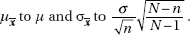
(f) More generally, what can be said about  if the population size N is very large?