DEFINITION
FOR A PROPORTION
FOR A DIFFERENCE OF TWO PROPORTIONS
FOR A MEAN
FOR A DIFFERENCE BETWEEN TWO MEANS
FOR THE SLOPE OF A LEAST SQUARES REGRESSION LINE
Using a measurement from a sample, we are never able to say exactly what a population proportion or mean is; rather we always say we have a certain confidence that the population proportion or mean lies in a particular interval. The particular interval is centered around a sample proportion or mean (or other statistic) and can be expressed as the sample estimate plus or minus an associated margin of error.
THE MEANING OF A CONFIDENCE INTERVAL
Using what we know about sampling distributions, we are able to establish a certain confidence that a sample proportion or mean lies within a specified interval around the population proportion or mean. However, we then have the same confidence that the population proportion or mean lies within a specified interval around the sample proportion or mean (e.g., the distance from Missoula to Whitefish is the same as the distance from Whitefish to Missoula).
Typically we consider 90%, 95%, and 99% confidence interval estimates, but any percentage is possible. The percentage is the percentage of samples that would pinpoint the unknown p or µ within plus or minus a certain margin or error. We do not say there is a 0.90, 0.95, or 0.99 probability that p or µ is within a certain margin of error of a given sample proportion or mean. For a given sample proportion or mean, p or µ either is or isn’t within the specified interval, and so the probability is either 1 or 0.
As will be seen, there are two aspects to this concept. First, there is the confidence interval, usually expressed in the form:
estimate ± margin of error
Second, there is the success rate for the method, that is, the proportion of times repeated applications of this method would capture the true population parameter.
CONFIDENCE INTERVAL FOR A PROPORTION
We are interested in estimating a population proportion p by considering a single sample proportion  . This sample proportion is just one of a whole universe of sample proportions, and from Topic 12 we remember the following:
1. The set of all sample proportions is approximately normally distributed.
2. The mean µ of the set of sample proportions equals p, the population proportion.
3. The standard deviation  of the set of sample proportions is approximately equal to
In finding confidence interval estimates of the population proportion p, how do we find  since p is unknown? The reasonable procedure is to use the sample proportion :

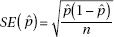
When the standard deviation is estimated in this way (using the sample), we use the term standard error. That is,
Remember that we are really using a normal approximation to the binomial, so n and n(1 – ) should both be at least 10. Furthermore, in making calculations and drawing conclusions from a specific sample, it is important that the sample be a simple random sample. Finally, the population should be large, typically checked by the assumption that the sample is less than 10% of the population. (If the population is small and the sample exceeds 10% of the population, then models other than the normal are more appropriate.)
 EXAMPLE 13.1
IMPORTANT
Verifying assumptions and conditions means more than simply listing them with little check marks. You must show work or give some reason to confirm verification.
If 64% of an SRS of 550 people leaving a shopping mall claim to have spent over $25, determine a 99% confidence interval estimate for the proportion of shopping mall customers who spend over $25.
Answer: We check that n = 550(0.64) = 352  10 and n(1 – ) = 550(0.36) = 198 10, we are given that the sample is an SRS, and it is reasonable to assume that 550 is less than 10% of all mall shoppers. Since = 0.64, the standard deviation of the set of sample proportions is
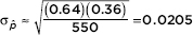
From Topic 11 we know that 99% of the sample proportions should be within 2.576 standard deviations of the population proportion. Equivalently, we are 99% certain that the population proportion is within 2.576 standard deviations of any sample proportion.1 Thus the 99% confidence interval estimate for the population proportion is 0.64 ± 2.576(0.0205) = 0.64 ± 0.053. We say that the margin of error is ±0.053. We are 99% certain that the proportion of shoppers spending over $25 is between 0.587 and 0.693.
We can also say, using the definition of confidence level, that if the interviewing procedure were repeated many times, about 99% of the resulting confidence intervals would contain the true proportion (thus we’re 99% confident that the method worked for the interval we got).1
TIP
The margin of error accounts for variation inherent in sampling, but it does not account for and is not a redress for bias in sampling.
EXAMPLE 13.2
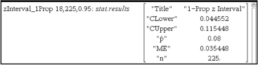
In a simple random sample of machine parts, 18 out of 225 were found to have been damaged in shipment. Establish a 95% confidence interval estimate for the proportion of machine parts that are damaged in shipment.
TIP
After finding a confidence interval, you must always interpret the interval in context.
Answer: We check that n = 18 10 and n(1 – ) = 225 – 18 = 207 10, we are given that the sample is an SRS, and it is reasonable to assume that 225 is less than 10% of all shipped machine parts.
Calculator software (such as 1-PropZInt on the TI-84) gives (0.04455,0.11545).
[For instructional purposes in this review book, we note that 

Thus we are 95% certain that the proportion of machine parts damaged in shipment is between 0.045 and 0.115.
On the TI-Nspire the result shows as:
Suppose there are 50,000 parts in the entire shipment. We can translate from proportions to actual numbers:
0.045(50,000) = 2250 and 0.115(50,000) = 5750
and so we can be 95% confident that there are between 2250 and 5750 defective parts in the whole shipment.
TIP
On the TI-84, for a confidence interval of a proportion, use 1-PropZInt, not Zinterval; and x must be an integer.
TIP
Finding confidence intervals using formulas is not necessary on free-response questions, but answer choices using formulas may well appear on multiple-choice questions.
EXAMPLE 13.3
A telephone survey of 1000 adults was taken shortly after the United States began bombing Iraq.
a. If 832 voiced their support for this action, with what confidence can it be asserted that 83.2% ± 3% of the adult U.S. population supported the decision to go to war?
Answer: We check that n = 832 10 and n(1 – ) = 1000 – 832 = 168 10, we assume an SRS, and clearly 1000 is <10% of the adult U.S. population.

The relevant z-scores are 
In other words, 83.2% ± 3% is a 98.89% confidence interval estimate for U.S. adult support of the war decision.
b. If the adult U.S. population is 191 million, estimate the actual numerical support.
Answer: Since
0.802(191,000,000) ≈ 153,000,000
while
0.862(191,000,000) ≈ 165,000,000
we can be 98.90% confident that between 153 and 165 million adults supported the initial bombing decision.
EXAMPLE 13.4
A U.S. Department of Labor survey of 6230 unemployed adults classified people by marital status, gender, and race. The raw numbers are as follows:
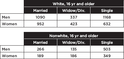
a. Find a 90% confidence interval estimate for the proportion of unemployed men who are married.
Answer: Totaling the first row across both tables, we find that there are 3499 men in the survey; 1090 + 266 = 1356 of them are married. We check that n = 1356 10 and n(1 – ) = 3499 – 1356 = 2143 10, we assume an SRS, and clearly the sample is <10% of the total unemployed adult population. On the TI-84, 1-PropZInt gives (0.37399, 0.40109). [For instructional purposes we note that  Thus the 90% confidence interval estimate is 0.3875 ± 1.645(0.008236) = 0.3875 ± 0.0135.] We are 90% confident that the true proportion of unemployed men who are married is between 0.374 and 0.401.
b. Find a 98% confidence interval estimate of the proportion of unemployed single persons who are women.
Answer: There are 1168 + 632 + 503 + 349 = 2652 singles in the survey. Of these, 632 + 349 = 981 are women [n = 981 10 and n(1 – ) = 2652 – 981 = 1671 10]. On the TI-84, 1-PropZInt gives (0.3481, 0.39172).
[For instructional purposes we note that 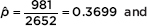
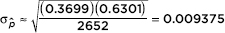
The 98% confidence interval estimate is 0.3699 ± 2.326(0.009375) = 0.3699 ± 0.0218.] We are 98% confident that the true proportion of unemployed single persons who are women is between 0.348 and 0.392.
As we have seen, there are two types of statements that come out of confidence intervals. First, we can interpret the confidence interval and say we are 90% confident that between 60% and 66% of all voters favor a bond issue. Second, we can interpret the confidence level and say that if this survey were conducted many times, then about 90% of the resulting confidence intervals would contain the true proportion of voters who favor the bond issue.
Incorrect statements include “The percentage of all voters who support the bond issue is between 60% and 66%,” “There is a 0.90 probability that the true percentage of all voters who favor the bond issue is between 60% and 66%,” and “If this survey were conducted many times, then about 90% of the sample proportions would be in the interval (0.60, 0.66).”
One important consideration in setting up a survey is the choice of sample size. To obtain a smaller, more precise interval estimate of the population proportion, we must either decrease the degree of confidence or increase the sample size. Similarly, if we want to increase the degree of confidence, we can either accept a wider interval estimate or increase the sample size. Again, while choosing a larger sample size may seem desirable, in the real world this decision involves time and cost considerations.
In setting up a survey to obtain a confidence interval estimate of the population proportion, what should we use for ? To answer this question, we first must consider how large  can be. We plot various values of p:

which gives 0.5 as the intuitive answer. Thus 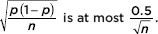 We make use of this fact to determine sample sizes in problems such as Examples 13.5 and 13.6.
TIP
Noting the inequality, the result must be rounded up if it is a decimal.
EXAMPLE 13.5
An Environmental Protection Agency (EPA) investigator wants to know the proportion of fish that are inedible because of chemical pollution downstream of an offending factory. If the answer must be within ±0.03 at the 96% confidence level, how many fish should be in the sample tested?
Answer: We want 2.05  0.03. From the above remark, is at most
  and so it is sufficient to consider 2.05
 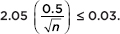 Algebraically, we have
 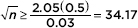 and n 1167.4. Therefore, choosing a sample of 1168 fish gives the inedible proportion to within ±0.03 at the 96% level.
Note that the accuracy of the estimate does not depend on what fraction of the whole population we have sampled. What is critical is the absolute size of the sample. Is some minimal value of n necessary for the procedures we are using to be meaningful? Since we are using the normal approximation to the binomial, both np and n(1 – p) should be at least 10 (see Topic 11).
EXAMPLE 13.6
A study is undertaken to determine the proportion of industry executives who believe that workers’ pay should be based on individual performance. How many executives should be interviewed if an estimate is desired at the 99% confidence level to within ±0.06? To within ±0.03? To within ±0.02?
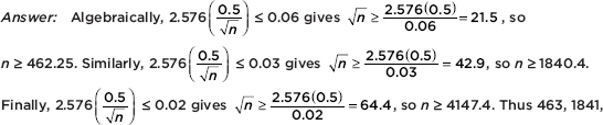
or 4148 executives should be interviewed, depending on the accuracy desired.
Note that to cut the interval estimate in half (from ±0.06 to ±0.03), we would have to increase the sample size fourfold, and to cut the interval estimate to a third (from ±0.06 to ±0.02), a ninefold increase in the sample size would be required (answers are not exact because of round-off error.)
More generally, to divide the interval estimate by d without affecting the confidence level, we must increase the sample size by a multiple of d2.
A formula for the calculations in Examples 13.5 and 13.6 is

(Note: this formula is not given on the AP Exam formula page.)
CONFIDENCE INTERVAL FOR A DIFFERENCE OF TWO PROPORTIONS
From Topic 12, we have the following information about the sampling distribution of 1 – 2:
1. The set of all differences of sample proportions is approximately normally distributed.
2. The mean of the set of differences of sample proportions equals p1 – p2, the difference of population proportions.
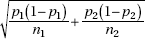
3. The standard deviation d of the set of differences of sample proportions is approximately equal to
Remember that we are using the normal approximation to the binomial, so n1 1, n1(1 – 1), n2 2, and n2(1 – 2) should all be at least 10. In making calculations and drawing conclusions from specific samples, it is important both that the samples be simple random samples and that they be taken independently of each other. Finally, the original populations should be large compared to the sample sizes.
EXAMPLE 13.7
Suppose that 84% of an SRS of 125 nurses working 7 a.m. to 3 p.m. shifts in city hospitals express positive job satisfaction, while only 72% of an SRS of 150 nurses on 11 p.m. to 7 a.m. shifts express similar fulfillment. Establish a 90% confidence interval estimate for the difference.
TIP
When interpreting the confidence interval for a difference, you must indicate which direction the difference is taken.
Answer: Note that n11 = (125)(0.84) = 105, n1(1 – 1) = (125)(0.16) = 20, n22 = (150)(0.72) = 108, and n2(1 – 2) = (150)(0.28) = 42 are all 10, we are given SRSs, and the population of city hospital nurses is assumed to be large. On the TI-84, 2-PropZInt gives (0.0391, 0.2009). [For instructional purposes, we note that
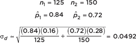
The observed difference is 0.84 – 0.72 = 0.12, and the critical z-scores are ±1.645. The confidence interval estimate is 0.12 ± 1.645(0.0492) = 0.12 ± 0.081.]
We can be 90% certain that the proportion of satisfied nurses on 7 a.m. to 3 p.m. shifts is between 0.039 and 0.201 higher than the proportion for nurses on 11 p.m. to 7 a.m. shifts.
EXAMPLE 13.8
A grocery store manager notes that in an SRS of 85 people going through the express checkout line, only 10 paid with checks, whereas, in an SRS of 92 customers passing through the regular line, 37 paid with checks. Find a 95% confidence interval estimate for the difference between the proportion of customers going through the two different lines who use checks.
Answer: Note that n1 1 = 10, n1(1 – 1) = 75, n2 2 = 37, and n2(1 – 2) = 55 are all at least 10, we are given SRSs, and the total number of customers is large. On the TI-84, 2-PropZInt gives (–0.4059, –0.1632). [For instructional purposes, we note that
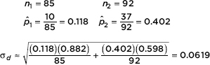
The observed difference is 0.118 – 0.402 = – 0.284, and the critical z-scores are ±1.96. Thus, the confidence interval estimate is – 0.284 ± 1.96(0.0619) = –0.284 ± 0.121.] The manager can be 95% sure that the proportion of customers passing through the express line who use checks is between 0.163 and 0.405 lower than the proportion going through the regular line who use checks.
With regard to choosing a sample size,  is at most 0.5. Thus
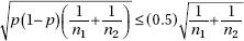
Now, if we simplify by insisting that n1 = n2 = n, the above statement can be reduced as follows:
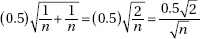
(Note: this formula is not given on the AP Exam formula page.)
EXAMPLE 13.9
A pollster wants to determine the difference between the proportions of high-income voters and low-income voters who support a decrease in the capital gains tax. If the answer must be known to within ±0.02 at the 95% confidence level, what size samples should be taken?
Answer: Assuming we will pick the same size samples for the two sample proportions, we have  Algebraically we find that
 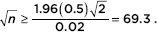 Therefore, n 69.32 = 4802.5, and the pollster should use 4803 people for each sample.
CONFIDENCE INTERVAL FOR A MEAN
We are interested in estimating a population mean µ by considering a single sample mean x. This sample mean is just one of a whole universe of sample means, and from Topic 12 we remember that if n is sufficiently large,
1. the set of all sample means is approximately normally distributed.
2. the mean of the set of sample means equals µ, the mean of the population.
3. the standard deviation x of the set of sample means is approximately equal to  that is, equal to the standard deviation of the whole population divided by the square root of the sample size.
Frequently we do not know , the population standard deviation. In such cases, we must use s, the standard deviation of the sample, as an estimate of . In this case  is called the standard error, SE(x), and is used as an estimate for x =
  (Note that we use t-distributions instead of the standard normal curve whenever is unknown, no matter what the sample size.)
Remember that in making calculations and drawing conclusions from a specific sample, it is important that the sample be a simple random sample and be no more than 10% of the population.
EXAMPLE 13.10
A bottling machine is operating with a standard deviation of 0.12 ounce. Suppose that in an SRS of 36 bottles the machine inserted an average of 16.1 ounces into each bottle.
a. Estimate the mean number of ounces in all the bottles this machine fills. More specifically, give an interval within which we are 95% certain that the mean lies.
Answer: For samples of size 36, the sample means are approximately normally distributed with a standard deviation of 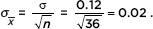 From Topic 11 we know that 95% of the sample means should be within 1.96 standard deviations of the population mean. Equivalently, we are 95% certain that the population mean is within 1.96 standard deviations of any sample mean. In our case, 16.1 ± 1.96(0.02) = 16.1 ± 0.0392, and we are 95% sure that the mean number of ounces in all bottles is between 16.0608 and 16.1392. This is called a 95% confidence interval estimate. [On the TI-84, under STAT and then TESTS, go to ZInterval. With Inpt:Stats, :.12, x:16.1, n:36, and C-Level:.95, Calculate gives (16.061, 16.139).]
b. How about a 99% confidence interval estimate?
Answer: Here, 16.1 ± 2.576(0.02) = 16.1 ± 0.0515, and we are 99% sure that the mean number of ounces in all bottles is between 16.0485 and 16.1515. [On the TI-84, ZInterval gives (16.048, 16.152).] We can also say, using the definition of confidence level, that if the sampling procedure were repeated many times, about 99% of the resulting confidence intervals would contain the true population mean (thus we’re 99% confident that the method worked for the interval we got).
Note that when we wanted a higher certainty (99% instead of 95%), we had to settle for a larger, less specific interval (±0.0515 instead of ±0.0392).
EXAMPLE 13.11
At a certain plant, batteries are being produced with a life expectancy that has a variance of 5.76 months squared. Suppose the mean life expectancy in an SRS of 64 batteries is 12.35 months.
a. Find a 90% confidence interval estimate of life expectancy for all the batteries produced at this plant.
Answer: The standard deviation of the population is 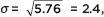 and the standard deviation of the sample means is
 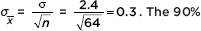 confidence interval estimate for the population mean is 12.35 ± 1.645(0.3) = 12.35 ± 0.4935. Thus we are 90% certain that the mean life expectancy of the batteries is between 11.8565 and 12.8435 months. [The TI-84 gives (11.857, 12.843).]
b. What would the 90% confidence interval estimate be if the sample mean of 12.35 had come from a sample of 100 batteries?
Answer: The standard deviation of the sample means would then have been 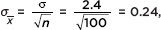 and the 90% confidence interval estimate would be 12.35 ± 1.645(0.24) = 12.35 ± 0.3948. [The TI-84 gives (11.955, 12.745).]
Note that when the sample size increased (from 64 to 100), the same sample mean resulted in a narrower, more specific interval (±0.3948 versus ±0.4935).
EXAMPLE 13.12
A new drug results in lowering the heart rate by varying amounts with a standard deviation of 2.49 beats per minute.
a. Find a 95% confidence interval estimate for the mean lowering of the heart rate in all patients if a 50-person SRS averages a drop of 5.32 beats per minute.
Answer: The standard deviation of sample means is 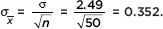 We are 95% certain that the mean lowering of the heart rate is in the range 5.32 ± 1.96(0.352) = 5.32 ± 0.69 or between 4.63 and 6.01 heartbeats per minute. [The TI-84 gives (4.6298, 6.0102).]
b. With what certainty can we assert that the new drug lowers the heart rate by a mean of 5.32 ± 0.75 beats per minute?
Answer: Converting ±0.75 to z-scores yields  From Table A, these z-scores give probabilities of 0.0166 and 0.9834, respectively, so our answer is 0.9834 – 0.0166 = 0.9668. In other words, 5.32 ± 0.75 beats per minute is a 96.68% confidence interval estimate of the mean lowering of the heart rate effected by this drug.
Remember, when is unknown (which is almost always the case), we use the t-distribution instead of the z-distribution. This follows if the parent population is normal (or at least nearly normal, which we can roughly check using a dotplot, stemplot, boxplot, histogram, or normal probability plot of the sample data), or if the sample size is large enough for the central limit theorem to apply. If we are not given that the parent population is normal, then for small samples (n ≤ 15) the sample data should be unimodal and symmetric with no outliers and no skewness; for medium samples (15 < n < 40) the sample data should be unimodal and reasonably symmetric with no extreme values and little, if any, skewness; while for large samples (n 40) the t-methods can be used no matter what the sample data show.
TIP
Understand that you are not trying to prove that the sample data are normal, but rather trying to infer something about the parent population.
EXAMPLE 13.13
When a random sample of 10 cars of a new model were tested for gas mileage, the results showed a mean of 27.2 miles per gallon with a standard deviation of 1.8 miles per gallon. What is a 95% confidence interval estimate for the gas mileage achieved by this model? (Assume that the population of mpg results for all the new model cars is approximately normally distributed.)
Answer: The sample is given to be random, 10 cars should be less than 10% of all cars of the new model, the population is approximately normal so the distribution of sample means is approximately normal, and a t-interval may be found. Calculator software (such as TInterval on the TI-84) gives (25.912, 28.488). [For instructional purposes we note that the standard deviation of the sample means is  = 0.569. With 10 – 1 = 9 degrees of freedom and 2.5% in each tail, the appropriate t-scores are ±2.262 (from Table B or InvT on the TI-84). Then 27 ± 2.262(0.569) = 27.2 ± 1.3.] We are 95% confident that the gas mileage of the new model is between 25.9 and 28.5 miles per gallon.
EXAMPLE 13.14
A new process for producing synthetic gems yielded six randomly selected stones weighing 0.43, 0.52, 0.46, 0.49, 0.60, and 0.56 carats, respectively, in its first run. Find a 90% confidence interval estimate for the mean carat weight from this process. (Assume that the population of carats of all gems produced by this new process is approximately normally distributed.)
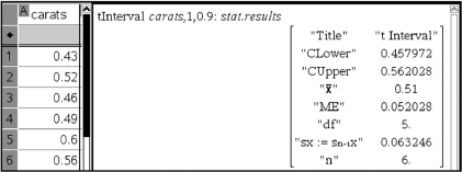
Answer: The sample is given to be random, six stones is assumed to be less than 10% of all stones produced by this process, the population is approximately normal so the distribution of sample means is approximately normal, and a t-interval may be found. Calculator software (such as TInterval on the TI-84 with the data put in a List) gives (0.45797, 0.56203). [For instructional purposes, we note that
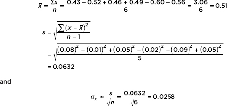
With df = 6 – 1 = 5 and 5% in each tail, the t-scores are ±2.015 (from Table B or InvT on the TI-84). Then 0.51 ± 2.015(0.0258) = 0.51 ± 0.052.] We are 90% confident that the mean carat weight for all stones produced by this procedure is between 0.458 and 0.562 carats.
On the TI-Nspire the result shows as:
TIP
Read the question carefully! Be sure you understand exactly what you are being asked to do or find or explain.
EXAMPLE 13.15
A survey was conducted involving 250 out of 125,000 families living in a city. The average amount of income tax paid per family in the sample was $3540 with a standard deviation of $1150. Establish a 99% confidence interval estimate for the total taxes paid by all the families in the city. (Assume that the population of all income taxes paid is approximately normally distributed.)
Answer: We are given x = 3540 and s = 1150. We use s as an estimate for s and calculate the standard deviation of the sample means to be 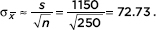
Since is unknown, we use a t-distribution. In this case we obtain 3540 ± 2.596(72.73) = 3540 ± 188.8 and then 125,000(3540 ± 188.8) = 442,500,000 ± 23,600,000. That is, we are 99% confident that the total tax paid by all families in the city is between $418,900,000 and $466,100,000.
Statistical principles are useful not only in analyzing data but also in setting up experiments, and one important consideration is the choice of a sample size. In making interval estimates of population means, we have seen that each inference must go hand in hand with an associated confidence level statement. Generally, if we want a smaller, more precise interval estimate, we either decrease the degree of confidence or increase the sample size. Similarly, if we want to increase the degree of confidence, we either accept a wider interval estimate or increase the sample size. Thus, choosing a larger sample size always seems desirable; in the real world, however, time and cost considerations are involved.
EXAMPLE 13.16
Ball bearings are manufactured by a process that results in a standard deviation in diameter of 0.025 inch. What sample size should be chosen if we wish to be 99% sure of knowing the diameter to within ±0.01 inch?
Answer: We have
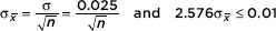
Thus
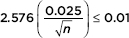
Algebraically, we find that
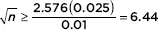
so n 41.5. We choose a sample size of 42.
A formula for the above calculation is

(Note: This formula is not given on the AP Exam formula page.)
Note that we can obtain a better estimate by recalculating using a t-score obtained from df = n – 1 where n is the value obtained from using the z-score. For example, in the above problem, a 99% confidence interval with df = 42 – 1 = 41 gives t = ±2.701. Then 2.701  results in n = 46.
TIP
Understand that you use a critical z-value here because to use a t-value you would need to know df, which is unknown without starting with a sample size.
CONFIDENCE INTERVAL FOR A DIFFERENCE BETWEEN TWO MEANS
We have the following information about the sampling distribution of x1 – x2:
1. The set of all differences of sample means is approximately normally distributed.
2. The mean of the set of differences of sample means equals µ1 – µ2, the difference of population means.
3. The standard deviation x1–x2 of the set of differences of sample means is approximately equal to 
In making calculations and drawing conclusions from specific samples, it is important both that the samples be simple random samples and that they be taken independently of each other.
EXAMPLE 13.17
A 30-month study is conducted to determine the difference in the numbers of accidents per month occurring in two departments in an assembly plant. Suppose the first department averages 12.3 accidents per month with a standard deviation of 3.5, while the second averages 7.6 accidents with a standard deviation of 3.4. Determine a 95% confidence interval estimate for the difference in the numbers of accidents per month. (Assume that the two populations are independent and approximately normally distributed.)
Answer: We are not given that the sample is random so must assume that the 30 months are representative. We are given that the two populations are independent and approximately normal, so the distributions of sample means are approximately normal, and a t-interval may be found. Calculator software (such as 2-SampTInt on the TI-84) gives (2.9167, 6.4833). [For instructional purposes we note
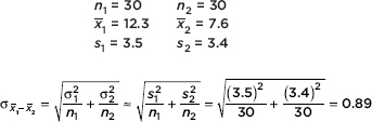
The observed difference is 12.3 – 7.6 = 4.7, and with df = (n1 – 1) + (n2 – 1) = 58, the critical t-scores are ±2.00. Thus the confidence interval estimate is 4.7 ± 2.00(0.89) = 4.7 ± 1.78.]
We are 95% confident that the first department has between 2.92 and 6.48 more accidents per month than the second department.
EXAMPLE 13.18
A hardware store owner wishes to determine the difference between the drying times of two brands of paint. Suppose the standard deviation between cans in each population is 2.5 minutes. How large a sample (same number) of each must the store owner use if he wishes to be 98% sure of knowing the difference to within 1 minute?
Answer:
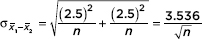
With a critical z-score of 2.326, we have 2.326 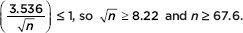 Thus the owner should test samples of 68 paint patches from each brand.
In the case of independent samples, there is also a procedure based on the assumption that both original populations not only are normally distributed but also have equal variances. Then we can get a better estimate of the common population variance by pooling the two sample variances. But it’s never wrong not to pool.
The analysis and procedure discussed in this section require that the two samples being compared be independent of each other. However, many experiments and tests involve comparing two populations for which the data naturally occur in pairs. In this case of paired differences, the proper procedure is to run a one-sample analysis on the single variable consisting of the differences from the paired data.
EXAMPLE 13.19
An SAT preparation class of 30 randomly selected students produces the following improvement in scores:
|
Student |
First Score |
Second Score |
Improvement |
|
1 |
912 |
1025 |
113 |
|
2 |
1025 |
1085 |
60 |
|
3 |
1295 |
1350 |
55 |
|
4 |
1123 |
1202 |
79 |
|
5 |
875 |
982 |
107 |
|
6 |
890 |
950 |
60 |
|
7 |
1002 |
1089 |
87 |
|
8 |
998 |
1159 |
161 |
|
9 |
1235 |
1246 |
11 |
|
10 |
1045 |
1135 |
90 |
|
11 |
956 |
1005 |
49 |
|
12 |
987 |
1010 |
23 |
|
13 |
1028 |
1015 |
–13 |
|
14 |
954 |
1032 |
78 |
|
15 |
1152 |
1310 |
158 |
|
16 |
1215 |
1302 |
87 |
|
17 |
948 |
1010 |
62 |
|
18 |
1190 |
1235 |
45 |
|
19 |
1077 |
1103 |
26 |
|
20 |
1223 |
1200 |
–23 |
|
21 |
1100 |
1187 |
87 |
|
22 |
842 |
910 |
68 |
|
23 |
985 |
1049 |
64 |
|
24 |
1107 |
1123 |
16 |
|
25 |
847 |
901 |
54 |
|
26 |
987 |
1086 |
99 |
|
27 |
1228 |
1276 |
48 |
|
28 |
1005 |
1029 |
24 |
|
29 |
1166 |
1221 |
55 |
|
30 |
808 |
874 |
66 |
Find a 90% confidence interval estimate of the average improvement in test scores.
Answer: We are given a random sample, and n = 30 is large enough so that by the CLT the distribution of sample means is approximately normal and a t-interval may be found. Putting the data (Improvement) into a List, calculator software (such as T-Interval on the TI-84) gives (50.206, 76.194). We are 90% confident that the average improvement in test scores is between 50.2 and 76.2.
When to do a two-sample analysis versus a matched pair analysis can be confusing. The key idea is whether or not the two groups are independent. The difference has to do with design. What is the average reaction time of people who are sober compared to that of people who have had two beers? If our experimental design calls for randomly assigning half of a group of volunteers to drink two beers and then comparing reaction times with the remaining sober volunteers, then a two-sample analysis is called for. However, if our experimental design calls for testing reaction times of all the volunteers and then giving all the volunteers two beers and retesting, then a matched pair analysis is called for. Matching may come about as above because you have made two measurements on the same person, or measurements might be made on sets of twins, or between salaries of president and provost at a number of universities, etc. The key is whether the two sets of measurements are independent, or related in some way relevant to the question under consideration.
TIP
Note the similarities between b1 ± t∗SE(b1),  ± z∗SE(), and x ± t∗SE(x).
CONFIDENCE INTERVAL FOR THE SLOPE OF A LEAST SQUARES REGRESSION LINE
In Topic 4 we discussed the least squares line
 = y + b1 (x – x)
where b1 is the slope of the line. This slope is readily found using the statistical software on a calculator. It is an estimate of the slope  of the true regression line. A confidence interval estimate for can be found using t-scores, where df = n – 2, and the appropriate standard deviation, the standard error of the slope, written sb1 or SE(b1), is
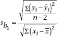
where the sum in the numerator is the sum of the squared residuals (see Topic 4) and the sum in the denominator is the sum of the squared deviations from the mean. The value of sb1 is found at the same time that the statistical software on your calculator finds the value of b1. Some calculators calculate the numerator  and then the denominator can be calculated by
Assumptions here include: (1) the sample must be randomly selected; (2) the scatterplot should be approximately linear; (3) there should be no apparent pattern in the residuals plot (On the TI-84, after Stat  Calc LinReg, the list of residuals is stored in RESID under LIST NAMES); and (4) the distribution of the residuals should be approximately normal. (The fourth point can be checked by a histogram, dotplot, stemplot, or a normal probability plot of the residuals.)
TIP
If you refer to a graph, whether it is a histogram, boxplot, stemplot, scatterplot, residuals plot, normal probability plot, or some other kind of graph, you should roughly draw it. It is not enough to simply say, “I did a normal probability plot of the residuals on my calculator and it looked linear.”
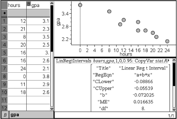
EXAMPLE 13.20
A random sample of ten high school students produced the following results for number of hours of television watched per week and GPA.
|
TV hours |
12 |
21 |
8 |
20 |
16 |
16 |
24 |
0 |
11 |
18 |
|
GPA |
3.1 |
2.3 |
3.5 |
2.5 |
3.0 |
2.6 |
2.1 |
3.8 |
2.9 |
2.6 |
Determine the least squares line and give a 95% confidence interval estimate for the true slope.
Answer: Checking the assumptions:
We are told that the data come from a random sample of students.

Now using the statistics software on a calculator gives
= 3.892 – 0.07202x
Putting the data into two Lists and using calculator software (such as LinRegTInt on the TI-84) gives (–0.0887, –0.0554).
We are thus 95% confident that each additional hour before the television each week is associated with between a 0.055 and a 0.089 drop in GPA.
On the TI-Nspire one can show the following:
Remember we must be careful about drawing conclusions concerning cause and effect; it is possible that students who have lower GPAs would have these averages no matter how much television they watched per week.
Note that  called the standard deviation of the residuals, is sometimes written se. It is a measure of the spread about the regression line, and is almost always in the regression output (usually simply labeled as s or S). Note that sb1 is sometimes written SE(b1) and is also referred to as the standard error of the slope. So we can also write
  We see that increasing se (that is, increasing spread about the line) increases the slope’s standard error, while increasing sx (that is, increasing the range of x-values) or increasing n (the sample size) decreases the slope’s standard error.
TIP
Practice how to read generic computer output, and note that you usually will not need to use all the information given.
EXAMPLE 13.21
Information concerning SAT verbal scores and SAT math scores was collected from 15 randomly selected subjects. A linear regression performed on the data using a statistical software package produced the following printout:
Dependent variable: Math
Variable |
Coef |
SE Coef |
T |
Prob |
Constant |
92.5724 |
31.75 |
2.92 |
0.012 |
Verbal |
0.763604 |
0.05597 |
13.6 |
0.000 |
S = 16.69 |
R–Sq = 93.5% |
R–Sq(adj) = 93.0% |
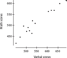
What is the regression equation?
Answer: Assuming that all assumptions for regression are met (we are given that the sample is random, and the scatterplot is approximately linear), the y-intercept and slope of the equation are found in the Coef column of the above printout.

What is a 95% confidence interval estimate for the slope of the regression line?
Answer: The standard deviation of the residuals is S = 16.69 and the standard error of the slope is Sb1 = 0.05597. With 15 data points, df = 15 – 2 = 13, and the critical t-values are ±2.160. The 95% confidence interval of the true slope is:
b1 ± t sb1 = 0.764 ± 2.160(0.05597) = 0.764 ± 0.121
We are 95% confident that for every 1-point increase in verbal SAT score, the average increase in math SAT score is between 0.64 and 0.89.
SUMMARY
 Important assumptions/conditions always must be checked before calculating confidence intervals.
We are never able to say exactly what a population parameter is; rather, we say that we have a certain confidence that it lies in a certain interval.
If we want a narrower interval, we must either decrease the confidence level or increase the sample size.
If we want a higher level of confidence, we must either accept a wider interval or increase the sample size.
The level of confidence refers to the percentage of samples that produce intervals that capture the true population parameter.
QUESTIONS ON TOPIC THIRTEEN: CONFIDENCE INTERVALS
Multiple-Choice Questions
Directions: The questions or incomplete statements that follow are each followed by five suggested answers or completions. Choose the response that best answers the question or completes the statement.
1. Changing from a 95% confidence interval estimate for a population proportion to a 99% confidence interval estimate, with all other things being equal,
(A) increases the interval size by 4%.
(B) decreases the interval size by 4%.
(C) increases the interval size by 31%.
(D) decreases the interval size by 31%.
(E) This question cannot be answered without knowing the sample size.
2. In general, how does doubling the sample size change the confidence interval size?
(A) Doubles the interval size
(B) Halves the interval size
(C) Multiplies the interval size by 1.414
(D) Divides the interval size by 1.414
(E) This question cannot be answered without knowing the sample size.
3. A confidence interval estimate is determined from the GPAs of a simple random sample of n students. All other things being equal, which of the following will result in a smaller margin of error?
(A) A smaller confidence level
(B) A larger sample standard deviation
(C) A smaller sample size
(D) A larger population size
(E) A smaller sample mean
4. A survey was conducted to determine the percentage of high school students who planned to go to college. The results were stated as 82% with a margin of error of ±5%. What is meant by ±5%?
(A) Five percent of the population were not surveyed.
(B) In the sample, the percentage of students who plan to go to college was between 77% and 87%.
(C) The percentage of the entire population of students who plan to go to college is between 77% and 87%.
(D) It is unlikely that the given sample proportion result would be obtained unless the true percentage was between 77% and 87%.
(E) Between 77% and 87% of the population were surveyed.
5. Most recent tests and calculations estimate at the 95% confidence level that the maternal ancestor to all living humans called mitochondrial Eve lived 273,000 ±177,000 years ago. What is meant by “95% confidence” in this context?
(A) A confidence interval of the true age of mitochondrial Eve has been calculated using z-scores of ±1.96.
(B) A confidence interval of the true age of mitochondrial Eve has been calculated using t-scores consistent with df = n – 1 and tail probabilities of ±.025.
(C) There is a .95 probability that mitochondrial Eve lived between 96,000 and 450,000 years ago.
(D) If 20 random samples of data are obtained by this method, and a 95% confidence interval is calculated from each, then the true age of mitochondrial Eve will be in 19 of these intervals.
(E) 95% of all random samples of data obtained by this method will yield intervals that capture the true age of mitochondrial Eve.
6. One month the actual unemployment rate in France was 13.4%. If during that month you took an SRS of 100 Frenchmen and constructed a confidence interval estimate of the unemployment rate, which of the following would have been true?
(A) The center of the interval was 13.4.
(B) The interval contained 13.4.
(C) A 99% confidence interval estimate contained 13.4.
(D) The z-score of 13.4 was between ±2.576.
(E) None of the above are true statements.
7. In a recent Zogby International survey, 11% of 10,000 Americans under 50 said they would be willing to implant a device in their brain to be connected to the Internet if it could be done safely. What is the margin of error at the 99% confidence level?
(A) 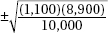
(B) 
(C) 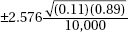
(D) 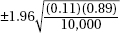
(E) 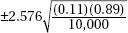
8. The margin of error in a confidence interval estimate using z-scores covers which of the following?
(A) Sampling variability
(B) Errors due to undercoverage and nonresponse in obtaining sample surveys
(C) Errors due to using sample standard deviations as estimates for population standard deviations
(D) Type I errors
(E) Type II errors
9. In an SRS of 50 teenagers, two-thirds said they would rather text a friend than call. What is the 98% confidence interval for the proportion of teens who would rather text than call a friend?
(A) 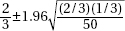
(B) 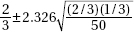
(C) 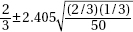
(D) 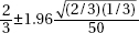
(E) 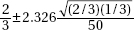
10. In a survey funded by Burroughs-Welcome, 750 of 1000 adult Americans said they didn’t believe they could come down with a sexually transmitted disease (STD). Construct a 95% confidence interval estimate of the proportion of adult Americans who don’t believe they can contract an STD.
(A) (0.728, 0.772)
(B) (0.723, 0.777)
(C) (0.718, 0.782)
(D) (0.713, 0.787)
(E) (0.665, 0.835)
11. A 1993 Los Angeles Times poll of 1703 adults revealed that only 17% thought the media was doing a “very good” job. With what degree of confidence can the newspaper say that 17% ± 2% of adults believe the media is doing a “very good” job?
(A) 72.9%
(B) 90.0%
(C) 95.0%
(D) 97.2%
(E) 98.6%
12. A politician wants to know what percentage of the voters support her position on the issue of forced busing for integration. What size voter sample should be obtained to determine with 90% confidence the support level to within 4%?
(A) 21
(B) 25
(C) 423
(D) 600
(E) 1691
13. In a New York Times poll measuring a candidate’s popularity, the newspaper claimed that in 19 of 20 cases its poll results should be no more than three percentage points off in either direction. What confidence level are the pollsters working with, and what size sample should they have obtained?
(A) 3%, 20
(B) 6%, 20
(C) 6%, 100
(D) 95%, 33
(E) 95%, 1068
14. In an SRS of 80 teenagers, the average number of texts handled in a day was 50 with a standard deviation of 15. What is the 96% confidence interval for the average number of texts handled by teens daily?
(A) 50 ± 2.054(15)
(B) 
(C) 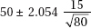
(D) 
(E) 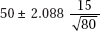
15. One gallon of gasoline is put in each of 30 test autos, and the resulting mileage figures are tabulated with x = 28.5 and s = 1.2. Determine a 95% confidence interval estimate of the mean mileage.
(A) (28.46, 28.54)
(B) (28.42, 28.58)
(C) (28.1, 28.9)
(D) (27.36, 29.64)
(E) (27.3, 29.7)
16. The number of accidents per day at a large factory is noted for each of 64 days with x = 3.58 and s = 1.52. With what degree of confidence can we assert that the mean number of accidents per day at the factory is between 3.20 and 3.96?
(A) 48%
(B) 63%
(C) 90%
(D) 95%
(E) 99%
17. A company owns 335 trucks. For an SRS of 30 of these trucks, the average yearly road tax paid is $9540 with a standard deviation of $1205. What is a 99% confidence interval estimate for the total yearly road taxes paid for the 335 trucks?
(A) $9540 ± $103
(B) $9540 ± $567
(C) $3,196,000 ± $606
(D) $3,196,000 ± $35,000
(E) $3,196,000 ± $203,000
18. What sample size should be chosen to find the mean number of absences per month for school children to within ±0.2 at a 95% confidence level if it is known that the standard deviation is 1.1?
(A) 11
(B) 29
(C) 82
(D) 96
(E) 117
19. Hospital administrators wish to learn the average length of stay of all surgical patients. A statistician determines that, for a 95% confidence level estimate of the average length of stay to within ±0.5 days, 50 surgical patients’ records will have to be examined. How many records should be looked at to obtain a 95% confidence level estimate to within ±0.25 days?
(A) 25
(B) 50
(C) 100
(D) 150
(E) 200
20. The National Research Council of the Philippines reported that 210 of 361 members in biology are women, but only 34 of 86 members in mathematics are women. Establish a 95% confidence interval estimate of the difference in proportions of women in biology and women in mathematics in the Philippines.
(A) 0.187 ± 0.115
(B) 0.187 ± 0.154
(C) 0.395 ± 0.103
(D) 0.543 ± 0.154
(E) 0.582 ± 0.051
21. In a simple random sample of 300 elderly men, 65% were married, while in an independent simple random sample of 400 elderly women, 48% were married. Determine a 99% confidence interval estimate for the difference between the proportions of elderly men and women who are married.
(A) 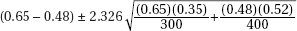
(B) 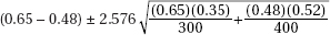
(C) 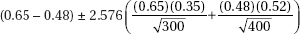
(D) 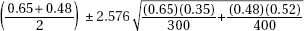
(E) 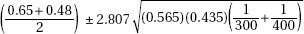
22. A researcher plans to investigate the difference between the proportion of psychiatrists and the proportion of psychologists who believe that most emotional problems have their root causes in childhood. How large a sample should be taken (same number for each group) to be 90% certain of knowing the difference to within ±0.03?
(A) 39
(B) 376
(C) 752
(D) 1504
(E) 3007
23. In a study aimed at reducing developmental problems in low-birth-weight (under 2500 grams) babies (Journal of the American Medical Association, June 13, 1990, page 3040), 347 infants were exposed to a special educational curriculum while 561 did not receive any special help. After 3 years the children exposed to the special curriculum showed a mean IQ of 93.5 with a standard deviation of 19.1; the other children had a mean IQ of 84.5 with a standard deviation of 19.9. Find a 95% confidence interval estimate for the difference in mean IQs of low-birth-weight babies who receive special intervention and those who do not.
(A) 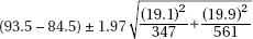
(B) 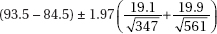
(C) 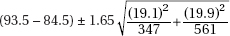
(D) 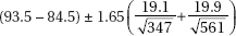
(E) 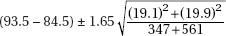
24. Does socioeconomic status relate to age at time of HIV infection? For 274 high-income HIV-positive individuals the average age of infection was 33.0 years with a standard deviation of 6.3, while for 90 low-income individuals the average age was 28.6 years with a standard deviation of 6.3 (The Lancet, October 22, 1994, page 1121). Find a 90% confidence interval estimate for the difference in ages of high- and low-income people at the time of HIV infection.
(A) 4.4 ± 0.963
(B) 4.4 ± 1.27
(C) 4.4 ± 2.51
(D) 30.8 ± 2.51
(E) 30.8 ± 6.3
25. An engineer wishes to determine the difference in life expectancies of two brands of batteries. Suppose the standard deviation of each brand is 4.5 hours. How large a sample (same number) of each type of battery should be taken if the engineer wishes to be 90% certain of knowing the difference in life expectancies to within 1 hour?
(A) 10
(B) 55
(C) 110
(D) 156
(E) 202
26. Two confidence interval estimates from the same sample are (16.4, 29.8) and (14.3, 31.9). What is the sample mean, and if one estimate is at the 95% level while the other is at the 99% level, which is which?
(A) x = 23.1; (16.4, 29.8) is the 95% level.
(B) x = 23.1; (16.4, 29.8) is the 99% level.
(C) It is impossible to completely answer this question without knowing the sample size.
(D) It is impossible to completely answer this question without knowing the sample standard deviation.
(E) It is impossible to completely answer this question without knowing both the sample size and standard deviation.
27. Two 90% confidence interval estimates are obtained: I (28.5, 34.5) and II (30.3, 38.2).
a. If the sample sizes are the same, which has the larger standard deviation?
b. If the sample standard deviations are the same, which has the larger size?
(A) a. Ib. I
(B) a. Ib. II
(C) a. IIb. I
(D) a. IIb. II
(E) More information is needed to answer these questions.
28. Suppose (25, 30) is a 90% confidence interval estimate for a population mean µ. Which of the following are true statements?
(A) There is a 0.90 probability that x is between 25 and 30.
(B) 90% of the sample values are between 25 and 30.
(C) There is a 0.90 probability that µ is between 25 and 30.
(D) If 100 random samples of the given size are picked and a 90% confidence interval estimate is calculated from each, then µ will be in 90 of the resulting intervals.
(E) If 90% confidence intervals are calculated from all possible samples of the given size, µ will be in 90% of these intervals.
29. Under what conditions would it be meaningful to construct a confidence interval estimate when the data consist of the entire population?
(A) If the population size is small (n < 30)
(B) If the population size is large (n 30)
(C) If a higher level of confidence is desired
(D) If the population is truly random
(E) Never
30. A social scientist wishes to determine the difference between the percentage of Los Angeles marriages and the percentage of New York marriages that end in divorce in the first year. How large a sample (same for each group) should be taken to estimate the difference to within ±0.07 at the 94% confidence level?
(A) 181
(B) 361
(C) 722
(D) 1083
(E) 1443
31. What is the critical t-value for finding a 90% confidence interval estimate from a sample of 15 observations?
(A) 1.341
(B) 1.345
(C) 1.350
(D) 1.753
(E) 1.761
32. Acute renal graft rejection can occur years after the graft. In one study (The Lancet, December 24, 1994, page 1737), 21 patients showed such late acute rejection when the ages of their grafts (in years) were 9, 2, 7, 1, 4, 7, 9, 6, 2, 3, 7, 6, 2, 3, 1, 2, 3, 1, 1, 2, and 7, respectively. Establish a 90% confidence interval estimate for the ages of renal grafts that undergo late acute rejection.
(A) 2.024 ± 0.799
(B) 2.024 ± 1.725
(C) 4.048 ± 0.799
(D) 4.048 ± 1.041
(E) 4.048 ± 1.725
33. Nine subjects, 87 to 96 years old, were given 8 weeks of progressive resistance weight training (Journal of the American Medical Association, June 13, 1990, page 3032). Strength before and after training for each individual was measured as maximum weight (in kilograms) lifted by left knee extension:
Before: |
3 |
3.5 |
4 |
6 |
7 |
8 |
8.5 |
12.5 |
15 |
After: |
7 |
17 |
19 |
12 |
19 |
22 |
28 |
20 |
28 |
Find a 95% confidence interval estimate for the strength gain.
(A) 11.61 ± 3.03
(B) 11.61 ± 3.69
(C) 11.61 ± 3.76
(D) 19.11 ± 1.25
(E) 19.11 ± 3.69
34. A catch of five fish of a certain species yielded the following ounces of protein per pound of fish: 3.1, 3.5, 3.2, 2.8, and 3.4. What is a 90% confidence interval estimate for ounces of protein per pound of this species of fish?
(A) 3.2 ± 0.202
(B) 3.2 ± 0.247
(C) 3.2 ± 0.261
(D) 4.0 ± 0.202
(E) 4.0 ± 0.247
35. In a random sample of 25 professional baseball players, their salaries (in millions of dollars) and batting averages result in the following regression analysis:
The regression equation is Batting = 0.234 + 0.00805 Salary
Predictor |
Coef |
SE Coef |
T |
P |
Constant |
0.233577 |
0.005883 |
39.70 |
0.000 |
Salary |
0.008051 |
0.001058 |
7.61 |
0.000 |
S = 0.0169461 R-Sq = 71.6% R-Sq(adj) = 70.3%
Which of the following gives a 98% confidence interval for the slope of the regression line?
(A) 0.008051 ± 2.326(0.001058)
(B) 0.008051 ± 2.326(0.0169461)
(C) 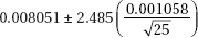
(D) 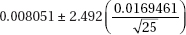
(E) 0.008051 ± 2.500(0.001058)
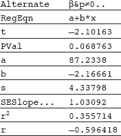
36. Is there a relationship between mishandled-baggage rates (number of mishandled bags per 1000 passengers) and percentage of on-time arrivals? Regression analysis of ten airlines gives the following TI-Nspire output (baggage rate is independent variable):
|
We are 95% confident that if an airline averages one more mishandled bag per 1000 passengers than a second airline, then its percentage of on-time arrivals will average |
(A) between 0.15 and 4.19 less than that of the second airline.
(B) between 0.00 and 4.33 less than that of the second airline.
(C) between 4.46 less and 0.13 more than that of the second airline.
(D) between 4.49 less and 0.17 more than that of the second airline.
(E) between 4.54 less and 0.21 more than that of the second airline.
37. Smoking is a known risk factor for cardiovascular and cancer diseases. A recent study (Rusanen et al., Archives of Internal Medicine, October 25, 2010) surveyed 21,123 members of a California health care system looking at smoking levels and risk of dementia (as measured by the Cox hazard ratio). Results are summarized in the following graph of 95% confidence intervals.
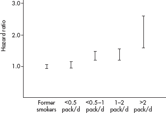
Which of the following is an appropriate conclusion?
(A) Dementia somehow causes an urge to smoke.
(B) Heavier smoking leads to a greater risk of dementia.
(C) Cutting down on smoking will lower one’s risk of dementia.
(D) Heavier smoking is associated with more precise confidence intervals of dementia as measured by the hazard ratio.
(E) There is a positive association between smoking and risk of dementia.
Free-Response Questions
Directions: You must show all work and indicate the methods you use. You will be graded on the correctness of your methods and on the accuracy of your final answers.
ELEVEN OPEN-ENDED QUESTIONS
1. An SRS of 1000 voters finds that 57% believe that competence is more important than character in voting for President of the United States.
(a) Determine a 95% confidence interval estimate for the percentage of voters who believe competence is more important than character.
(b) If your parents know nothing about statistics, how would you explain to them why you can’t simply say that 57% of voters believe that competence is more important.
(c) Also explain to your parents what is meant by 95% confidence level.
2. During the H1N1 pandemic, one published study concluded that if someone in your family had H1N1, you had a 1 in 8 chance of also coming down with the disease. A state health officer tracks a random sample of new H1N1 cases in her state and notes that 129 out of a potential 876 family members later come down with the disease.
(a) Calculate a 90% confidence interval for the proportion of family members who come down with H1N1 after an initial family member does in this state.
(b) Based on this confidence interval, is there evidence that the proportion of family members who come down with H1N1 after an initial family member does in this state is different from the 1 in 8 chance concluded in the published study? Explain.
(c) Would the conclusion in (b) be any different with a 99% confidence interval? Explain.
3. In a random sample of 500 new births in the United States, 41.2% were to unmarried women, while in a random sample of 400 new births in the United Kingdom, 46.5% were to unmarried women.
(a) Calculate a 95% confidence interval for the difference in the proportions of new births to unmarried women in the United States and United Kingdom.
(b) Does the confidence interval support the belief by a UN health care statistician that the proportions of new births to unmarried women is different in the United States and United Kingdom? Explain.
4. An SRS of 40 inner city gas stations shows a mean price for regular unleaded gasoline to be $3.45 with a standard deviation of $0.05, while an SRS of 120 suburban stations shows a mean of $3.38 with a standard deviation of $0.08.
(a) Construct 95% confidence interval estimates for the mean price of regular gas in inner city and in suburban stations.
(b) The confidence interval for the inner city stations is wider than the interval for the suburban stations even though the standard deviation for inner city stations is less than that for suburban stations. Explain why this happened.
(c) Based on your answer in part (a), are you confident that the mean price of inner city gasoline is less than $3.50? Explain.
5. In a simple random sample of 30 subway cars during rush hour, the average number of riders per car was 83.5 with a standard deviation of 5.9. Assume the sample data are unimodal and reasonably symmetric with no extreme values and little, if any, skewness.
(a) Establish a 90% confidence interval estimate for the average number of riders per car during rush hour. Show your work.
(b) Assuming the same standard deviation of 5.9, how large a sample of cars would be necessary to determine the average number of riders to within ±1 at the 90% confidence level? Show your work.
6. In a sample of ten basketball players the mean income was $196,000 with a standard deviation of $315,000.
(a) Assuming all necessary assumptions are met, find a 95% confidence interval estimate of the mean salary of basketball players.
(b) What assumptions are necessary for the above estimate? Do they seem reasonable here?
7. An SRS of ten brands of breakfast cereals is tested for the number of calories per serving. The following data result: 185, 190, 195, 200, 205, 205, 210, 210, 225, 230.
Establish a 95% confidence interval estimate for the mean number of calories for servings of breakfast cereals. Be sure to check assumptions.
8. Bisphenol A (BPA), a synthetic estrogen found in packaging materials, has been shown to leach into infant formula and beverages. Most recently it has been detected in high concentrations in cash register receipts. Random sample biomonitoring data to see if retail workers carry higher amounts of BPA in their bodies than non-retail workers is as follows:
|
|
BPA concentration (µg/L) |
|
|
Sample size |
Mean |
Standard deviation |
|
Non-retail workers |
528 |
2.43 |
0.45 |
|
Retail workers |
197 |
3.28 |
0.48 |
(a) Calculate a 99% confidence interval for the difference in mean BPA body concentrations of non-retail and retail workers.
(b) Does the confidence interval support the belief that retail workers carry higher amounts of BPA in their bodies than non-retail workers? Explain.
9. A new drug is tested for relief of allergy symptoms. In a double-blind experiment, 12 patients are given varying doses of the drug and report back on the number of hours of relief. The following table summarizes the results:
|
Dosage (mg) |
2 |
3 |
4 |
4 |
5 |
6 |
6 |
7 |
8 |
8 |
9 |
10 |
|
Duration of relief (hrs) |
3 |
7 |
6 |
8 |
10 |
8 |
13 |
16 |
15 |
21 |
23 |
24 |
(a) Determine the equation of the least squares regression line.
(b) Construct a 90% confidence interval estimate for the slope of the regression line, and interpret this in context.
10. Information with regard to the assessed values (in $1000) and the selling prices (in $1000) of a random sample of homes sold in an NE market yields the following computer output:
Dependent variable isPrice
R squared = 89.8% R squared (adjusted) = 89.2%
s = 9.508 with 20 – 2 = 18 degrees of freedom
Source |
SS |
df |
MS |
F-ratio |
Regression |
14271.2 |
1 |
14271.2 |
158 |
Residual |
1627.31 |
18 |
90.4063 |
|
Variable |
Coeff |
s.e. of coeff |
t-ratio |
prob |
Constant |
0.890087 |
16.16 |
0.055 |
0.956 |
Assessed |
1.0292 |
0.08192 |
12.6 |
0.000 |
(a) Determine the equation of the least squares regression line.
(b) Construct a 99% confidence interval estimate for the slope of the regression line, and interpret this in context.
11. In a July 2008 study of 1050 randomly selected smokers, 74% said they would like to give up smoking.
(a) At the 95% confidence level, what is the margin of error?
(b) Explain the meaning of “95% confidence interval” in this example.
(c) Explain the meaning of “95% confidence level” in this example.
(d) Give an example of possible response bias in this example.
(e) If we want instead to be 99% confident, would our confidence interval need to be wider or narrower?
(f) If the sample size were greater, would the margin of error be smaller or greater?
AN INVESTIGATIVE TASK
As of January 1, 2014, Serena Williams had career prize money earnings of $54,380,000 during her 18 year professional career. Among the top active women tennis players, is there a linear relationship between career prize money earnings and years as a pro? Computer output of earnings (millions of $) versus professional years for 10 top active women players are shown below:
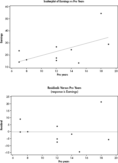
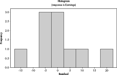
Regression Analysis: Earnings versus Pro Years
Predictor |
Coef |
SE Coef |
T |
P |
Constant |
2.69 |
10.78 |
0.25 |
0.809 |
Pro Years |
1.6752 |
0.8264 |
2.03 |
0.077 |
S = 10.5317 R-Sq = 33.9% R-Sq(adj) = 25.7%
Analysis of Variance
Source |
DF |
SS |
MS |
F |
P |
Regression |
1 |
455.8 |
455.8 |
4.11 |
0.077 |
Residual Error |
8 |
887.3 |
110.9 |
|
|
Total |
9 |
1343.1 |
|
|
|
(a) Determine the equation of the least squares regression line.
(b) Comment on the strength of the linear relationship.
(c) Predict the career earnings for Years = 15 and Years = 30 for active women tennis players, and explain your confidence in both of your answers.
(d) Find the 90% confidence interval for the slope of the regression line, and interpret in context.
(e) Assuming all conditions for inference are met, and using a t-distribution with df = n – 2, find the 90% confidence interval for the y-intercept, and if appropriate, interpret in context. Explain.
(f) A second linear model is found: = 1.8712(Years). Explain why you might prefer this model to the one in (a).
1 Note that we cannot say there is a 0.99 probability that the population proportion is within 2.576 standard deviations of a given sample proportion. For a given sample proportion, the population proportion either is or isn’t within the specified interval, and so the probability is either 1 or 0.