
14 Tests of Significance—Proportions and Means
 LOGIC OF SIGNIFICANCE TESTING
NULL AND ALTERNATIVE HYPOTHESES
P-VALUES
TYPE I AND TYPE II ERRORS
CONCEPT OF POWER
HYPOTHESIS TESTING
Closely related to the problem of estimating a population proportion or mean is the problem of testing a hypothesis about a population proportion or mean. For example, a travel agency might determine an interval estimate for the proportion of sunny days in the Virgin Islands or, alternatively, might test a tourist bureau’s claim about the proportion of sunny days. A major stockholder in a construction company might ascertain an interval estimate for the proportion of successful contract bids or, alternatively, might test a company spokesperson’s claim about the proportion of successful bids. A consumer protection agency might determine an interval estimate for the mean nicotine content of a particular brand of cigarettes or, alternatively, might test a manufacturer’s claim about the mean nicotine content of its cigarettes. An agricultural researcher could find an interval estimate for the mean productivity gain caused by a specific fertilizer or, alternatively, might test the developer’s claimed mean productivity gain. In each of these cases, the experimenter must decide whether the interest lies in an interval estimate of a population proportion or mean or in a hypothesis test of a claimed proportion or mean.
LOGIC OF SIGNIFICANCE TESTING, NULL AND ALTERNATIVE HYPOTHESIS, P-VALUES, ONE- AND TWO-SIDED TESTS, TYPE I AND TYPE II ERRORS, AND THE CONCEPT OF POWER
The general testing procedure is to choose a specific hypothesis to be tested, called the null hypothesis, pick an appropriate random sample, and then use measurements from the sample to determine the likelihood of the null hypothesis. If the sample statistic is far enough away from the claimed population parameter, we say that there is sufficient evidence to reject the null hypothesis. We attempt to show that the null hypothesis is unacceptable by showing that it is improbable.
Consider the context of the population proportion. The null hypothesis H0 is stated in the form of an equality statement about the population proportion (for example, H0: p = 0.37). There is an alternative hypothesis, stated in the form of an inequality (for example, Ha: p < 0.37 or Ha: p > 0.37 or Ha: p ≠ 0.37). The strength of the sample statistic  can be gauged through its associated P-value, which is the probability of obtaining a sample statistic as extreme (or more extreme) as the one obtained if the null hypothesis is assumed to be true. The smaller the P-value, the more significant the difference between the null hypothesis and the sample results.
TIP
Never base your hypotheses on what you find in the sample data.
Note that only population parameter symbols appear in H0 and Ha. Sample statistics like x and do NOT appear in H0 or Ha.
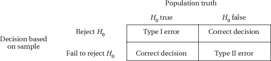
There are two types of possible errors: the error of mistakenly rejecting a true null hypothesis and the error of mistakenly failing to reject a false null hypothesis. The  -risk, also called the significance level of the test, is the probability of committing a Type I error and mistakenly rejecting a true null hypothesis. A Type II error, a mistaken failure to reject a false null hypothesis, has associated probability
  . There is a different value of for each possible correct value for the population parameter p. For each , 1 – is called the power of the test against the associated correct value. The power of a hypothesis test is the probability that a Type II error is not committed. That is, given a true alternative, the power is the probability of rejecting the false null hypothesis. Increasing the sample size and increasing the significance level are both ways of increasing the power.
TIP
The P-value relates to the probability of the data given that the null hypothesis is true; it is not the probability of the null hypothesis being true.
A simple illustration of the difference between a Type I and a Type II error is as follows: Suppose the null hypothesis is that all systems are operating satisfactorily with regard to a NASA liftoff. A Type I error would be to delay the liftoff mistakenly thinking that something was malfunctioning when everything was actually OK. A Type II error would be to fail to delay the liftoff mistakenly thinking everything was OK when something was actually malfunctioning. The power is the probability of recognizing a particular malfunction. (Note the complimentary aspect of power, a “good” thing, with Type II error, a “bad” thing.)
TIP
Understand that the sample statistic almost never equals the claimed population parameter. Either the sample statistic differs by random chance, or the claimed parameter is wrong.
Our justice system provides another often quoted illustration. If the null hypothesis is that a person is innocent, then a Type I error results when an innocent person is found guilty, while a Type II error results when a guilty person is not convicted. We try to minimize Type I errors in criminal trials by demanding unanimous jury guilty verdicts. In civil suits, however, many states try to minimize Type II errors by accepting simple majority verdicts.
It should be emphasized that with regard to calculations, questions like “What is the power of this test?” and “What is the probability of a Type II error in this test?” cannot be answered without reference to a specific alternative hypothesis. Furthermore, AP students are not required to know how to calculate these probabilities. However, they are required to understand the concepts and interactions among the concepts.
TIP
Be able to identify Type I and Type II errors and give possible consequences of each.
HYPOTHESIS TEST FOR A PROPORTION
We must check that we have a simple random sample, that both np0 and n(1 – p0) are at least 10, and that the sample size is less than 10% of the population.
TIP
Always check assumptions/conditions before proceeding with a test.
 EXAMPLE 14.1
A union spokesperson claims that 75% of union members will support a strike if their basic demands are not met. A company negotiator believes the true percentage is lower and runs a hypothesis test. What is the conclusion if 87 out of an SRS of 125 union members say they will strike?
Answer: We note that np0 = (125)(0.75) = 93.75 and n(1 – p0) = (125)(0.25) = 31.25 are both  10 and that we have an SRS, and we assume that 125 is less than 10% of the total union membership.

TIP
Hypotheses are always about the population, never about a sample; note H0 is p = 0.75, not = 0.75.
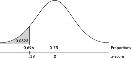
Calculator software (such as 1-PropZTest on the TI-84) gives z = –1.394 and P = 0.0816. [For instructional purposes in this review book, we note that the observed sample proportion is 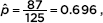 and using the claimed proportion, 0.75, we have
  with a resulting P-value of 0.0817.]
TIP
Always give a conclusion in context.
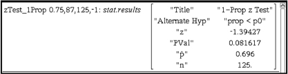
There are two possible answers: With this large a P-value, 0.0816 > 0.05, there is not sufficient evidence to reject H0, that is, there is not sufficient evidence that the true percentage of union members who support a strike is less than 75%.
OR With this small a P-value, 0.0816 < 0.10, there is sufficient evidence to reject H0, that is, there is sufficient evidence that the true percentage of union members who support a strike is less than 75%.
TIP
We never “accept” a null hypothesis; we either do or do not have evidence to reject it.
On the TI-Nspire the result shows as:
TIP
Although performing hypotheses tests using formulas is not necessary on free-response questions, answer choices using formulas may well appear on multiple-choice questions.
TIP
If the question does not suggest a direction for the alternative, then use a two-sided test.
EXAMPLE 14.2
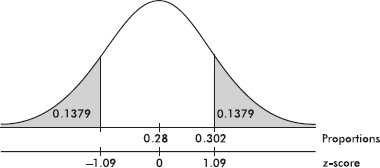
A cancer research group surveys a random sample of 500 women more than 40 years old to test the hypothesis that 28% of women in this age group have regularly scheduled mammograms. Should the hypothesis be rejected at the 5% significance level if 151 of the women respond affirmatively?
Answer: Note that np0 = (500)(0.28) = 140 and n(1 – p0) = (500)(0.72) = 360 are both 10, we are given a random sample, and clearly 500 < 10% of all women over 40 years old. Since no suspicion is voiced that the 28% claim is low or high, we run a two-sided z-test for proportions:

TIP
Remember: when we fail to reject H0, we are not accepting it; it simply means that there is not sufficient evidence against H0, that is, we cannot rule out random chance as the explanation.
Calculator software (such as 1-PropZTest on the TI-84) gives z = 1.0956 and P = 0.2732. [For instructional purposes, we note that the observed 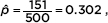
 which corresponds to a tail probability of 0.1366. Doubling this value (because the test is two-sided) gives a P-value of 0.2732.] With this large a P-value, 0.2732 > 0.05, there is not sufficient evidence to reject H0, that is, the cancer research group should not dispute the 28% claim.
HYPOTHESIS TEST FOR A DIFFERENCE BETWEEN TWO PROPORTIONS
As with confidence intervals for the difference of two proportions, n11, n1(1 – 1), n22, and n2(1 – 2) should all be at least 10, it is important both that the samples be simple random samples and that they be taken independently of each other, and the original populations should be large compared to the sample sizes.
TIP
The samples must be independent to use these two sample proportion methods.
The fact that a sample proportion from one population is greater than a sample proportion from a second population does not automatically justify a similar conclusion about the population proportions themselves. Two points need to be stressed. First, sample proportions from the same population can vary from each other. Second, what we are really comparing are confidence interval estimates, not just single points.
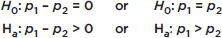
For many problems the null hypothesis states that the population proportions are equal or, equivalently, that their difference is 0:
H0: p1 – p2 = 0
The alternative hypothesis is then
Ha: p1 – p2 < 0 Ha: p1 – p2 > 0 or Ha: p1 – p2 ≠ 0
where the first two possibilities lead to one-sided tests and the third possibility leads to two-sided tests.
Since the null hypothesis is that p1 = p2, we call this common value p and use this pooled value in calculating  d:
d:
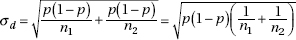
In practice, if 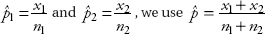 as an estimate of p in calculating d.
TIP
This is the one situation where it is necessary to use a pooled proportion.
EXAMPLE 14.3
Suppose that early in an election campaign a telephone poll of 800 randomly chosen registered voters shows 460 in favor of a particular candidate. Just before election day, a second poll shows only 520 of 1000 randomly chosen registered voters expressing the same preference. Is there sufficient evidence that the candidate’s popularity has decreased?
Answer: Note that n1 1 = 460, n1(1 – 1) = 340, n2 2 = 520, and n2(1 – 2) = 480 are all at least 10 (where n1 and 1 refer to the first poll, ,and n2 and 2 refer to the second poll), we are given that the samples are random and independent by design, and clearly the total population of registered voters is large.
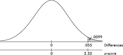
Calculator software (such as 2-PropZTest on the TI-84) gives z = 2.328 and P = 0.00995. [For instructional purposes, we note that the observed difference is 0.575 – 0.520 = 
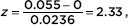 and the tail probability gives P = 0.0099.] With this small a P-value, 0.00995 < 0.05, there is sufficient evidence to reject H0, that is, there is sufficient evidence that the candidate’s popularity has dropped.
TIP
Along with the P-value, you should also give the test statistic, as we have been doing.
EXAMPLE 14.4
An automobile manufacturer tries two distinct assembly procedures. In a random sample of 350 cars coming off the line using the first procedure there are 28 with major defects, while a random sample of 500 autos from the second line shows 32 with defects. Is the difference significant at the 10% significance level?
Answer: Note that n1 1 = 28, n1(1 – 1) = 322, n2 2 = 32, and n2(1 – 2) = 468 are all at least 10 (where n1 and 1 refer to the sample of cars using the first procedure, and n2 and 2 refer to the sample of cars using the second procedure), we are given that the samples are random and independent by design, and the total population of autos manufactured at the plant is large. Since there is no mention that one procedure is believed to be better or worse than the other, this is a two-sided test.
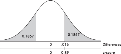
Calculator software (such as 2-PropZTest on the TI-84) gives z = 0.8963 and P = 0.3701. [For instructional purposes, we note that the observed difference is 0.080 – 0.064 = 
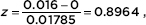 which corresponds to a tail probability of 0.1850. Doubling this value (because the test is two-sided) gives a P-value of 0.3700.] With this large a P-value, 0.3700 > 0.05, there is not sufficient evidence to reject H0, that is, there is not sufficient evidence of a significant difference in proportions of cars with major defects coming from the two assembly procedures.
We must check that we have a simple random sample, that the sample size is less than 10% of the population, and that the distribution of sample means is approximately normal, which follows if either the sample size is large enough for the CLT to apply or the population has an approximately normal distribution (if we are given the sample data, we check the normality assumption with a graph such as a histogram or a normal probability plot: the histogram should be unimodal and reasonably symmetric, although this condition can be relaxed the larger the sample size.)
EXAMPLE 14.5
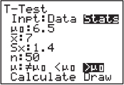
A manufacturer claims that a new brand of air-conditioning unit uses only 6.5 kilowatts of electricity per day. A consumer agency believes the true figure is higher and runs a test on a random sample of size 50. If the sample mean is 7.0 kilowatts with a standard deviation of 1.4, should the manufacturer’s claim be rejected at a significance level of 5%? Of 1%?
Answer: We are given a random sample, n = 50 is large enough for the CLT to apply so the distribution of sample means is approximately normal, and we can assume that 50 is less than 10% of all of the new AC units. The population SD is unknown, so a t-test is called for with H0: μ = 6.5 and Ha: μ > 6.5. Calculator software (such as T-Test on the TI-84) gives t = 2.525 and P = 0.0074. [For instructional purposes, we note that 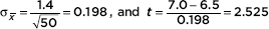 with a resulting P-value of 0.0074.] With this small a P-value, 0.0074 < 0.05, there is sufficient evidence to reject H0, that is, there is sufficient evidence for the consumer agency to reject the manufacturer’s claim that the new unit uses a mean of only 6.5 kilowatts of electricity per day.
EXAMPLE 14.6
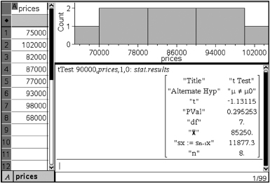
A local chamber of commerce claims that the mean sale price for homes in the city is $90,000. A real estate salesperson notes a random sample of eight recent sales of $75,000, $102,000, $82,000, $87,000, $77,000, $93,000, $98,000, and $68,000. How strong is the evidence to reject the chamber of commerce claim?
Answer: We are given a random sample, we can assume n = 8 is less than 10% of all home sales, and we check for normality with a histogram, which yields the roughly unimodal, roughly symmetric:

The population SD is unknown, so a t-test is called for with H0: μ = 90,000 and Ha: μ ≠ 90,000. Putting the data into a List, calculator software (such as T-Test on the TI-84) gives t = –1.131 and P = 0.2953. With such a large P-value, 0.2953 > 0.05, there is not sufficient evidence to reject H0, that is, there is not sufficient evidence to reject the commerce claim of a mean sale price of $90,000 for homes in the city.
On the TI-Nspire the result shows as:
HYPOTHESIS TEST FOR A DIFFERENCE BETWEEN TWO MEANS (UNPAIRED AND PAIRED)
We assume that we have two independent simple random samples, each from an approximately normally distributed population (the normality assumptions can be relaxed if the sample sizes are large).
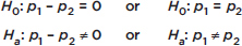
In this situation the null hypothesis is usually that the means of the populations are the same or, equivalently, that their difference is 0:
H0: µ1 – µ2 = 0
The alternative hypothesis is then
Ha: µ1 – µ2 < 0 Ha: µ1 – µ2 > 0 or Ha: µ1 – µ2 ≠ 0
The first two possibilities lead to one-sided tests, and the third possibility leads to two-sided tests.
EXAMPLE 14.7
A sales representative believes that his company’s computer has more average downtime per week than a similar computer sold by a competitor. Before taking this concern to his director, the sales representative gathers data and runs a hypothesis test. He determines that in a simple random sample of 40 week-long periods at different firms using his company’s product, the average downtime was 125 minutes with a standard deviation of 37 minutes. However, 35 week-long periods involving the competitor’s computer yield an average downtime of only 115 minutes with a standard deviation of 43 minutes. What conclusion should the sales representative draw?
TIP
Avoid “calculator speak.” For example, do not simply write “2-SampTTest…” or “binomcdf…” There are lots of calculators out there, each with its own abbreviations.
Answer: We are given independent SRSs, the sample sizes can be assumed to be less than 10% of all possible weeks and are large enough to relax the normality assumptions. The population SDs are unknown, so a t-test is called for with
H0: µ1 – µ2 = 0 (where µ1 = mean down time of company’s computers
Hα: µ1 – µ2 > 0 and µ2 = mean down time of competitor’s computers)
Calculator software (such as 2-SampTTest on the TI-84) gives t = 1.0718 and P = 0.1438. With this large a P-value, 0.1438 > 0.05, there is not sufficient evidence to reject H0, that is, the sales representative does not have sufficient evidence that his company’s computers have greater mean downtime than that of the competitor’s computers.
TIP
While the normal probability plot is not part of the AP Stat curriculum, it is useful and is accepted on the exam.
EXAMPLE 14.8
A city council member claims that male and female officers wait equal times for promotion in the police department. A women’s spokesperson, however, believes women must wait longer than men. If a random sample of five men waited 8, 7, 10, 5, and 7 years, respectively, for promotion while a random sample of four women waited 9, 5, 12, and 8 years, respectively, what conclusion should be drawn?
Answer: We are given random samples and must assume they are independent and less than 10% of total numbers of male and female officers. These samples are too small for histograms to show anything other than no outliers, but the normal probability plots are fairly linear indicating that it is not unreasonable to assume the data come from roughly normal distributions:
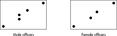
The population SDs are unknown, so a t-test is called for with H0: µM = µF and Hα: µM < µF. Putting the data into Lists, calculator software (such as 2-SampTTest on the TI-84) gives t = –0.6641 and P = 0.2685. With this large a P-value, 0.2685 > 0.05, there is not sufficient evidence to reject H0, that is, there is not sufficient evidence to dispute the council member’s claim that male and female officers wait equal times for promotion.
The analysis and procedure described above require that the two samples being compared be independent of each other. However, many experiments and tests involve comparing two populations for which the data naturally occur in pairs. In this case, the proper procedure is to run a one-sample test on a single variable consisting of the differences from the paired data.
EXAMPLE 14.9
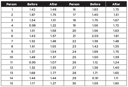
Does a particular drug slow reaction times? If so, the government might require a warning label concerning driving a car while taking the medication. An SRS of 30 people who might benefit from the drug are tested before and after taking the drug, and their reaction times (in seconds) to a standard testing procedure are noted. The resulting data are as follows:
TIP
When the data comes in pairs, you cannot use a two sample t-test.
We can calculate the mean reaction times before and after, 1.46 seconds and 1.50 seconds, respectively, and ask if this observed rise is significant. If we performed a two-sample test, we would calculate the P-value to be 0.2708 and would conclude that with such a large P, the observed rise is not significant. However, this would not be the proper test or conclusion! The two-sample test works for independent sets. However, in this case, there is a clear relationship between the data, in pairs, and this relationship is completely lost in the procedure for the two-sample test. The proper procedure is to form the set of 30 differences, being careful with signs, {–0.06, 0.12, 0.03, –0.24, …}, and to perform a single sample hypothesis test as follows:
Name the test:
We are using a paired t-test, that is, a single sample hypothesis test on the set of differences.
State the hypothesis:
H0: The reaction times of individuals to a standard testing procedure are the same before and after they take a particular drug; the mean difference is zero: µd = 0.
Ha: The reaction time is greater after they take the drug; the mean difference is less than zero: µd < 0.
Check the conditions:
1. The data are paired because they are measurements on the same individuals before and after taking the drug.
2. The reaction times of any individual are independent of the reaction times of the others, so the differences are independent.
3. A random sample of people are tested.
4. The histogram of the differences looks nearly normal (roughly unimodal and symmetric):
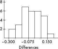
5. The sample size, n = 30, is less than 10% of the population of all people who may take the drug.
Perform the mechanics:
Putting the data into lists, say L1 and L2, then L1 – L2 Æ L3, calculator software (such as T-Test on the TI-84) on the data in L3 gives t = –1.755 with P = 0.0449. [For instructional purposes, we note that a calculator readily gives: n = 30, x = –0.037667, and s = 0.11755.
Then 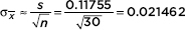 and
and
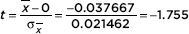
With df = n – 1 = 29, the P-value is P(t < –1.755) = 0.0449.]
Give a conclusion in context:
With this small a P-value, 0.0449 < 0.05, there is sufficient evidence to reject H0, that is, there is sufficient evidence that the mean observed rise in reaction times after taking the drug is significant.
MORE ON POWER AND TYPE II ERRORS
Given a specific alternative hypothesis, a Type II error is a mistaken failure to reject the false null hypothesis, while the power is the probability of rejecting that false null hypothesis.
EXAMPLE 14.10
A candidate claims to have the support of 70% of the people, but you believe that the true figure is lower. You plan to gather an SRS and will reject the 70% claim if in your sample shows 65% or less support. What if in reality only 63% of the people support the candidate?
TIP
You will not have to calculate actual probabilities of Type II errors or power.
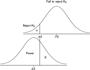
The upper graph shows the null hypothesis model with the claim that p0 = 70, and the plan to reject H0 if < 0.65. The lower graph shows the true model with p = 0.63. When will we fail to pick up that the null hypothesis is incorrect? Answer: precisely when the sample proportion is greater than 0.65. This is a Type II error with probability . When will we rightly conclude that the null hypothesis is incorrect? Answer: when the sample proportion is less than 0.65. This is the power of the test and has probability 1 – .
TIP
While calculations are not called for, you must understand the interactions among the errors, confidence level, power, effect, and sample size.
The following points should be emphasized:
 Power gives the probability of avoiding a Type II error.
Power has a different value for different possible correct values of the population parameter; thus it is actually a function where the independent variable ranges over specific alternative hypotheses.
Choosing a smaller (that is, a tougher standard to reject H0) results in a higher risk of Type II error and a lower power—observe in the above graphs how making smaller (in this case moving the critical cutoff value to the left) makes the power less and more!
The greater the difference between the null hypothesis p0 and the true value p, the smaller the risk of a Type II error and the greater the power—observe in the above picture how moving the lower graph to the left makes the power greater and less. (The difference between p0 and p is sometimes called the effect—thus the greater the effect, the greater is the power to pick it up.)
A larger sample size n will reduce the standard deviations, making both graphs narrower resulting in smaller , smaller , and larger power!
TIP
Both blocking in experiments and stratification in sampling reduce variability and so can improve power.
CONFIDENCE INTERVALS VERSUS HYPOTHESIS TESTS
A question sometimes arises as to whether a problem calls for calculating a confidence interval or performing a hypothesis test. Generally, a claim about a population parameter indicates a hypothesis test, while an estimate of a population parameter asks for a confidence interval. However, some confusion may arise because sometimes it is possible to conduct a hypothesis test by constructing a confidence interval estimate of the parameter and then checking whether or not the null parameter value is in the interval. While, when possible, this alternative approach is accepted on the AP exam, it does require very special care in still remembering to state hypotheses, in dealing with one-sided versus two-sided, and in how standard errors are calculated in problems involving proportions. So the recommendation is to conduct a hypothesis test like a hypothesis test. Carefully read the question. If it asks whether or not there is evidence, then this is a hypothesis test; if it involves how much or how effective, then this is a confidence interval calculation. However, it should be noted that there have been AP free-response questions where part (a) calls for a confidence interval calculation and part (b) asks if this calculation provides evidence relating to a hypothesis test.
SUMMARY
Important assumptions/conditions always must be checked before proceeding with a hypothesis test.
The null hypothesis is stated in the form of an equality statement about a population parameter, while the alternative hypothesis is in the form of an inequality.
We attempt to show that a null hypothesis is unacceptable by showing it is improbable.
The P-value is the probability of obtaining a sample statistic as extreme (or more extreme) as the one obtained if the null hypothesis is assumed to be true.
When the P-value is small (typically, less than 0.05 or 0.10), we say we have evidence to reject the null hypothesis.
A Type I error is the probability of mistakenly rejecting a true null hypothesis.
A Type II error is the probability of mistakenly failing to reject a false null hypothesis.
The power of a hypothesis test is the probability that a Type II error is not committed.
QUESTIONS ON TOPIC FOURTEEN: TESTS OF SIGNIFICANCE—PROPORTIONS AND MEANS
Multiple-Choice Questions
Directions: The questions or incomplete statements that follow are each followed by five suggested answers or completions. Choose the response that best answers the question or completes the statement.
1. Which of the following is a true statement?
(A) A well-planned hypothesis test should result in a statement either that the null hypothesis is true or that it is false.
(B) The alternative hypothesis is stated in terms of a sample statistic.
(C) If a sample is large enough, the necessity for it to be a simple random sample is diminished.
(D) When the null hypothesis is rejected, it is because it is not true.
(E) Hypothesis tests are designed to measure the strength of evidence against the null hypothesis.
2. Which of the following is a true statement?
(A) The P-value of a test is the probability of obtaining a result as extreme (or more extreme) as the one obtained assuming the null hypothesis is false.
(B) If the P-value for a test is 0.015, the probability that the null hypothesis is true is 0.015.
(C) The larger the P-value, the more evidence there is against the null hypothesis.
(D) If possible, always examine your data before deciding whether to use a one-sided or two-sided hypothesis test.
(E) The alternative hypothesis is one-sided if there is interest in deviations from the null hypothesis in only one direction.
Questions 3–4 refer to the following:
Video arcades provide a vehicle for competition and status within teenage peer groups and are recognized as places where teens can hang out and meet their friends. The national PTA organization, concerned about the time and money being spent in video arcades by middle school students, commissions a statistical study to investigate whether or not middle school students are spending an average of over two hours per week in video arcades. Twenty communities are randomly chosen, five middle schools are randomly picked in each of the communities, and ten students are randomly interviewed at each school.
3. What is the parameter of interest?
(A) Video arcades
(B) A particular concern of the national PTA organization
(C) 1000 randomly chosen middle school students
(D) The mean amount of money spent in video arcades by middle school students
(E) The mean number of hours per week spent in video arcades by middle school students
4. What are the null and alternative hypotheses which the PTA is testing?
(A) H0: µ = 2Ha: µ < 2
(B) H0: µ = 2Ha: µ ≤ 2
(C) H0: µ = 2Ha: µ > 2
(D) H0: µ = 2Ha: µ 2
(E) H0: µ = 2Ha: µ ≠ 2
5. A hypothesis test comparing two population proportions results in a P-value of 0.032. Which of the following is a proper conclusion?
(A) The probability that the null hypothesis is true is 0.032.
(B) The probability that the alternative hypothesis is true is 0.032.
(C) The difference in sample proportions is 0.032.
(D) The difference in population proportions is 0.032.
(E) None of the above are proper conclusions.
6. A company manufactures a synthetic rubber (jumping) bungee cord with a braided covering of natural rubber and a minimum breaking strength of 450 kg. If the mean breaking strength of a sample drops below a specified level, the production process is halted and the machinery inspected. Which of the following would result from a Type I error?
(A) Halting the production process when too many cords break.
(B) Halting the production process when the breaking strength is below the specified level.
(C) Halting the production process when the breaking strength is within specifications.
(D) Allowing the production process to continue when the breaking strength is below specifications.
(E) Allowing the production process to continue when the breaking strength is within specifications.
7. One ESP test asks the subject to view the backs of cards and identify whether a circle, square, star, or cross is on the front of each card. If p is the proportion of correct answers, this may be viewed as a hypothesis test with H0: p = 0.25 and Ha: p > 0.25. The subject is recognized to have ESP when the null hypothesis is rejected. What would a Type II error result in?
(A) Correctly recognizing someone has ESP
(B) Mistakenly thinking someone has ESP
(C) Not recognizing that someone really has ESP
(D) Correctly realizing that someone doesn’t have ESP
(E) Failing to understand the nature of ESP
8. A coffee-dispensing machine is supposed to deliver 12 ounces of liquid into a large paper cup, but a consumer believes that the actual amount is less. As a test he plans to obtain a sample of 5 cups of the dispensed liquid and if the mean content is less than 11.5 ounces, to reject the 12-ounce claim. If the machine operates with a known standard deviation of 0.9 ounces, what is the probability that the consumer will mistakenly reject the 12-ounce claim even though the claim is true?
(A) 0.054
(B) 0.107
(C) 0.214
(D) 0.289
(E) 0.393
9. A pharmaceutical company claims that a medicine will produce a desired effect for a mean time of 58.4 minutes. A government researcher runs a hypothesis test of 40 patients and calculates a mean of x = 59.5 with a standard deviation of s = 8.3. What is the P-value?
(A) 
(B) 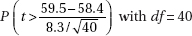
(C) 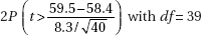
(D) 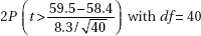
(E) 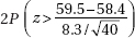
10. You plan to perform a hypothesis test with a level of significance of = 0.05. What is the effect on the probability of committing a Type I error if the sample size is increased?
(A) The probability of committing a Type I error decreases.
(B) The probability of committing a Type I error is unchanged.
(C) The probability of committing a Type I error increases.
(D) The effect cannot be determined without knowing the relevant standard deviation.
(E) The effect cannot be determined without knowing if a Type II error is committed.
11. A fast food chain advertises that their large bag of french fries has a weight of 150 grams. Some high school students, who enjoy french fries at every lunch, suspect that they are getting less than the advertised amount. With a scale borrowed from their physics teacher, they weigh a random sample of 15 bags. What is the conclusion if the sample mean is 145.8 g and standard deviation is 12.81 g?
(A) There is sufficient evidence to prove the fast food chain advertisement is true.
(B) There is sufficient evidence to prove the fast food chain advertisement is false.
(C) The students have sufficient evidence to reject the fast food chain’s claim.
(D) The students do not have sufficient evidence to reject the fast food chain’s claim.
(E) There is not sufficient data to reach any conclusion.
12. A researcher believes a new diet should improve weight gain in laboratory mice. If ten control mice on the old diet gain an average of 4 ounces with a standard deviation of 0.3 ounces, while the average gain for ten mice on the new diet is 4.8 ounces with a standard deviation of 0.2 ounces, what is the P-value?
(A) 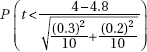
(B) 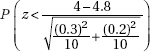
(C) 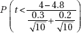
(D) 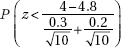
(E) 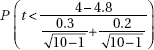
13. A school superintendent must make a decision whether or not to cancel school because of a threatening snow storm. What would the results be of Type I and Type II errors for the null hypothesis: The weather will remain dry?
(A) Type I error: don’t cancel school, but the snow storm hits.
Type II error: weather remains dry, but school is needlessly canceled.
(B) Type I error: weather remains dry, but school is needlessly canceled.
Type II error: don’t cancel school, but the snow storm hits.
(C) Type I error: cancel school, and the storm hits.
Type II error: don’t cancel school, and weather remains dry.
(D) Type I error: don’t cancel school, and snow storm hits.
Type II error: don’t cancel school, and weather remains dry.
(E) Type I error: don’t cancel school, but the snow storm hits.
Type II error: cancel school, and the storm hits.
14. A pharmaceutical company claims that 8% or fewer of the patients taking their new statin drug will have a heart attack in a 5-year period. In a government-sponsored study of 2300 patients taking the new drug, 198 have heart attacks in a 5-year period. Is this strong evidence against the company claim?
(A) Yes, because the P-value is 0.005657.
(B) Yes, because the P-value is 0.086087.
(C) No, because the P-value is only 0.005657.
(D) No, because the P-value is only 0.086087.
(E) No, because the P-value is over 0.10.
15. Is Internet usage different in the Middle East and Latin America? In a random sample of 500 adults in the Middle East, 151 claimed to be regular Internet users, while in a random sample of 1000 adults in Latin America, 345 claimed to be regular users. What is the P-value for the appropriate hypothesis test?
(A) 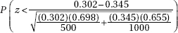
(B) 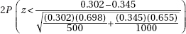
(C) 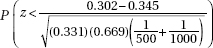
(D) 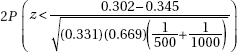
(E) 2(0.095167)
16. What is the probability of mistakenly failing to reject a false null hypothesis when a hypothesis test is being conducted at the 5% significance level ( = 0.05)?
(A) 0.025
(B) 0.05
(C) 0.10
(D) 0.95
(E) There is insufficient information to answer this question.
17. A research dermatologist believes that cancers of the head and neck will occur most often of the left side, the side next to a window when a person is driving. In a review of 565 cases of head/neck cancers, 305 occurred on the left side. What is the resulting p-value?
(A) 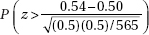
(B) 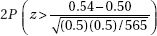
(C) 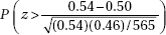
(D) 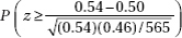
(E) 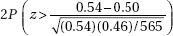
18. Suppose you do five independent tests of the form H0: µ = 38 versus Ha: µ > 38, each at the = 0.01 significance level. What is the probability of committing a Type I error and incorrectly rejecting a true null hypothesis with at least one of the five tests?
(A) 0.01
(B) 0.049
(C) 0.05
(D) 0.226
(E) 0.951
19. Given an experiment with H0: µ = 35, Ha: µ < 35, and a possible correct value of 32, you obtain a sample statistic of x = 33. After doing analysis, you realize that the sample size n is actually larger than you first thought. Which of the following results from reworking with the increase in sample size?
(A) Decrease in probability of a Type I error; decrease in probability of a Type II error; decrease in power.
(B) Increase in probability of a Type I error; increase in probability of a Type II error; decrease in power.
(C) Decrease in probability of a Type I error; decrease in probability of a Type II error; increase in power.
(D) Increase in probability of a Type I error; decrease in probability of a Type II error; decrease in power.
(E) Decrease in probability of a Type I error; increase in probability of a Type II error; increase in power.
20. Thirty students volunteer to test which of two strategies for taking multiple-choice exams leads to higher average results. Each student flips a coin, and if heads, uses Strategy A on the first exam and then Strategy B on the second, while if tails, uses Strategy B first and then Strategy A. The average of all 30 Strategy A results is then compared to the average of all 30 Strategy B results. What is the conclusion at the 5% significance level if a two-sample hypothesis test, H0: µ1 = µ2, Ha: µ1 ≠ µ2, results in a P-value of 0.18?
(A) The observed difference in average scores is significant.
(B) The observed difference in average scores is not significant.
(C) A conclusion is not possible without knowing the average scores resulting from using each strategy.
(D) A conclusion is not possible without knowing the average scores and the standard deviations resulting from using each strategy.
(E) A two-sample hypothesis test should not be used here.
21. Choosing a smaller level of significance, that is, a smaller -risk, results in
(A) a lower risk of Type II error and lower power.
(B) a lower risk of Type II error and higher power.
(C) a higher risk of Type II error and lower power.
(D) a higher risk of Type II error and higher power.
(E) no change in risk of Type II error or in power.
22. The greater the difference between the null hypothesis claim and the true value of the population parameter,
(A) the smaller the risk of a Type II error and the smaller the power.
(B) the smaller the risk of a Type II error and the greater the power.
(C) the greater the risk of a Type II error and the smaller the power.
(D) the greater the risk of a Type II error and the greater the power.
(E) the greater the probability of no change in Type II error or in power.
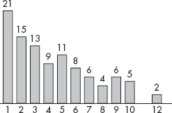
23. A company selling home appliances claims that the accompanying instruction guides are written at a 6th grade reading level. An English teacher believes that the true figure is higher and with the help of an AP Statistics student runs a hypothesis test. The student randomly picks one page from each of 25 of the company’s instruction guides, and the teacher subjects the pages to a standard readability test. The reading levels of the 25 pages are given in the following table:

Is there statistical evidence to support the English teacher’s belief?
(A) No, because the P-value is greater than 0.10.
(B) Yes, the P-value is between 0.05 and 0.10 indicating some evidence for the teacher’s belief.
(C) Yes, the P-value is between 0.01 and 0.05 indicating evidence for the teacher’s belief.
(D) Yes, the P-value is between 0.001 and 0.01 indicating strong evidence for the teacher’s belief.
(E) Yes, the P-value is less than 0.001 indicating very strong evidence for the teacher’s belief.
24. Suppose H0: p = 0.4, and the power of the test for the alternative hypothesis p = 0.35 is 0.75. Which of the following is a valid conclusion?
(A) The probability of committing a Type I error is 0.05.
(B) The probability of committing a Type II error is 0.65.
(C) If the alternative p = 0.35 is true, the probability of failing to reject H0 is 0.25.
(D) If the null hypothesis is true, the probability of rejecting it is 0.25.
(E) If the null hypothesis is false, the probability of failing to reject it is 0.65.
25. A factory is located close to a city high school. The manager claims that the plant’s smokestacks spew forth an average of no more than 350 pounds of pollution per day. As an AP Statistics project, the class plans a one-sided hypothesis test with a critical value of 375 pounds. Suppose the standard deviation in daily pollution poundage is known to be 150 pounds and the true mean is 385 pounds. If the sample size is 100 days, what is the probability that the class will mistakenly fail to reject the factory manager’s false claim?
(A) 0.0475
(B) 0.2525
(C) 0.7475
(D) 0.7514
(E) 0.9525
Free-Reponse Questions
Directions: You must show all work and indicate the methods you use. You will be graded on the correctness of your methods and on the accuracy of your final answers.
TEN OPEN-ENDED QUESTIONS
1. Next to good brakes, proper tire pressure is the most crucial safety issue on your car. Incorrect tire pressure compromises cornering, braking, and stability. Both underinflation and overinflation can lead to problems. The number on the tire is the maximum allowable air pressure—not the recommended pressure for that tire. At a roadside vehicle safety checkpoint, officials randomly select 30 cars for which 35 psi is the recommended tire pressure and calculate the average of the actual tire pressure in the front right tires. What is the parameter of interest, and what are the null and alternative hypotheses that the officials are testing?
2. No vaccinations are 100% risk free, and the theoretical risk of rare complications always have to be balanced against the severity of the disease. Suppose the CDC decides that a risk of one in a million is the maximum acceptable risk of GBS (Guillain-Barre syndrome) complications for a new vaccine for a particularly serious strain of influenza. A large sample study of the new vaccine is conducted with the following hypotheses:
H0: The proportion of GBS complications is 0.000001 (one in a million)
Ha: The proportion of GBS complications is greater than 0.000001 (one in a million)
The P-value of the test is 0.138.
(a) Interpret the P-value in context of this study.
(b) What conclusion should be drawn at the = 0.10 significance level?
(c) Given this conclusion, what possible error, Type I or Type II, might be committed, and give a possible consequence of committing this error.
3. A particular wastewater treatment system aims at reducing the most probable number per ml (MPN/ml) of E. coli to 1000 MPN/100 ml. A random study of 40 of these systems in current use is conducted with the data showing a mean of 1002.4 MPN/100 ml and a standard deviation of 7.12 MPN/100 ml. A test of significance is conducted with:
H0: The mean concentration of E. coli after treatment under this system is 1000 MPN/100 ml.
Ha: The mean concentration of E. coli after treatment under this system is greater than 1000 MPN/100 ml.
The resulting P-value is 0.0197 with df = 39 and t = 2.132.
(a) Interpret the P-value in context of this study.
(b) What conclusion should be drawn at a 5% significance level?
(c) Given this conclusion, what possible error, Type I or Type II, might be committed, and give a possible consequence of committing this error.
4. A 20-year study of 5000 British adults noted four bad habits: smoking, drinking, inactivity, and poor diet. The study looked to show that there is a higher death rate (proportion who die in a 20-year period) among people with all four bad habits than among people with none of the four bad habits.
(a) Was this an experiment or observational study? Explain.
(b) What are the null and alternative hypotheses?
(c) What would be the result of a Type I error?
(d) What would be the result of a Type II error?
Of the 314 people who had all four bad habits, 91 died during the study, while of the 387 people with none of the four bad habits, 32 died during the study.
(e) Calculate and interpret the P-value in context of this study.
5. It is estimated that 17.4% of all U.S. households own a Roth IRA. The American Association of University Professors (AAUP) believes this figure is higher among their members and commissions a study. If 150 out of a random sample of 750 AAUP members own Roth IRAs, is this sufficient evidence to support the AAUP belief?
6. A long accepted measure of the discharge rate (in 1000 ft3/sec) at the mouth of the Mississippi River is 593. To test if this has changed, ten measurements at random times are taken: 590, 596, 592, 588, 589, 594, 590, 586, 591, 589. Is there statistical evidence of a change?
7. A behavior study of high school students looked at whether a higher proportion of boys than girls met a recommended level of physical activity (increased heart rate for 60 minutes/day for at least 5 days during the 7 days before the survey). What is the proper conclusion if 370 out of a random sample of 850 boys and 218 out of an independent random sample of 580 girls met the recommended level of activity?
8. In a random sample of 35 NFL games the average attendance was 68,729 with a standard deviation of 6,110, while in a random sample of 30 Big 10 Conference football games the average attendance was 70,358 with a standard deviation of 9,139. Is there evidence that the average attendance at Big 10 Conference football games is greater than that at NFL games?
9. A study is proposed to compare two treatments for patients with significantly narrowed neck arteries. Some patients will be treated with surgery to remove built-up plaque, while others will be treated with stents to improve circulation. The response variable will be the proportion of patients who suffer a major complication such as a stroke or heart attack within one month of the treatment. The researchers decide to block on whether or not a patient has had a mini stroke in the previous year.
(a) There are 1000 patients available for this study, half of whom have had a mini stroke in the previous year. Explain a block design to assign patients to treatments.
(b) Give two methods other than blocking to increase the power of detecting a difference between using surgery versus stents for patients with this medical condition. Explain your choice of methods.
10. A car simulator was used to compare effect on reaction time between DWI (driving while intoxicated) and DWT (driving while texting). Ten volunteers were instructed to drive at 50 mph and then hit the brakes in response to the sudden image of a child darting into the road. A baseline stopping distance was established for each driver. Then one day each driver was tested for stopping distance while driving while texting, and another day the driver was tested after consuming a quantity of alcohol. For each driver, which test was done on the first day was decided by coin toss. The following table gives the extra number of feet necessary to stop at 50 mph for each driver for DWI and DWT.

The sample means are xDWI = 32.2, xDWT = 33.6, and a two-sample t-test, H0: µDWI = µDWT, Ha: µDWI ≠ µDWT, gives a P-value of 0.590, and a conclusion that there is no evidence of a difference between the effect on reaction time between DWI and DWT. Explain why this is not the proper hypothesis test, and then perform the proper test.
SIX INVESTIGATIVE TASKS
1. An exercise electrocardiogram (EKG) checks for changes in your heart during exercise and is useful in diagnosing coronary artery disease. An EKG has fewer potential side effects but is much less precise than thallium tomography. In one EKG study, 500 volunteers with known coronary artery disease and 500 volunteers with healthy arteries underwent EKG checks. The physicians administering and evaluating the tests did not know the physical condition of any volunteer. The following table gives the numbers of volunteers whom the physicians evaluated as “positive” for coronary disease.
|
Test for coronary disease |
|
|
Positive |
Negative |
|
|
Healthy volunteers |
100 |
400 |
|
Volunteers with disease |
305 |
195 |
(a) Sensitivity is defined as the probability of a positive test given that the subject has disease. What was the sensitivity of this study?
(b) Specificity is defined as the probability of a negative test given that the subject is healthy. What was the specificity of this study?
(c) A valuable tool for assessing the accuracy of such studies is the positive diagnostic likelihood ratio (LR+) which gives the ratio of the probability a positive test result will be observed in a diseased person compared to the probability that the same result will be observed in a healthy person.
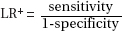
What was LR+ in this study, and explain why the larger the value of LR+, the more useful the test.
(d) Suppose in one such sample study, LR+ = 4.7. To determine whether or not this is sufficient evidence that the population LR+ is below the desired value of 5.0, 100 samples from a population with a known LR+ of 5.0 are generated, and the resulting simulated values of LR+ are shown in the dotplot:
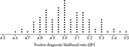
Based on this dotplot and the sample LR+ = 4.7, is there evidence that the population LR+ is below the desired value of 5.0? Explain.
2. An engineer wishes to test which of two drills can more quickly bore holes in various materials. He assembles a random sampling of ten materials of various hardnesses and thicknesses.
(a) Given that a drill’s efficiency is influenced by how long and how hard it has been operating, the engineer decided to randomly choose the order in which the materials will be tested. Design and implement a scheme to place the materials in random order using the following random number table:
51844 73424 84380 82259 28273 58102 18727 69708
(b) Suppose the drilling times (in seconds) are summarized as follows:
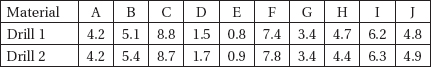
What is the mean drilling time for each drill? Is the difference significant? Justify your answer.
3. Paul the octopus, who lives in a tank at Sea Life Centre in Oberhausen, Germany, correctly predicted the winner in 12 out of 14 soccer matches (by choosing to eat mussels from the boxes labeled with national flags of the eventual winning teams). Assume these 14 matches represent a random sample of matches which Paul could predict, and assume that all matches end in a win for one of the teams (using sudden death overtime or penalty kicks to settle tie scores from regulation time).
(a) Why would it be incorrect to perform a one-sample z-test on whether the above is sufficient evidence that Paul can correctly predict the results of more than 50% of soccer matches?
(b) Perform a proper hypothesis test for the question in (a).
4. A marketing company is interested in whether a particular advertisement will increase interest in a new social networking website. A random sample of 15 teenagers is chosen, and their interest level in the new website is measured on a 1–100 scale before and after seeing the advertisement. The individual results are as follows:

(a) The ad developer claims that after seeing the ad, the interest level is above 30. Do the data support this conclusion? Explain.
(b) The ad developer also claims that after seeing the ad, teenagers have increased interest in the new website. Assuming all assumptions for hypothesis testing are met, do the data support this conclusion? Explain.
(c) Can after-ad interest level be predicted from before-ad interest level? Explain.
(d) Can the change in interest level be predicted by before-ad interest level? Explain.
5. According to one national survey, 20% of 18–24-year-olds have passports.
(a) Assuming the 20% figure is correct, use simulation to determine the approximate probability that in a random sample of ten 18–24-year-olds, at least three have passports.
2498346851 4113296825 1485367833 8663018872 7373275392
5062790330 2367029195 4153038298 7360048279 4207598980
9574649262 4488086249 2651769472 9462095309 4072555345
7894788460 2391904958 0201791131 9856022851 1405559336
6003121057 4154811850 7697586849 9644852135 0811348895
(b) Calculate the above probability exactly.
(c) Suppose you believe that the 20% claim is too high and run a hypothesis test. In a simple random sample of 200 18–24-year-olds you find only 33 who have passports. Is this sufficient evidence to dispute the 20% claim?
(d) If the 20% claim is true, what is the probability that the first 18–24-year-old with a passport will be the third one sampled?
(e) A 100-trial simulation is performed to determine the number of 18–24-year-olds sampled before finding one with a passport. The results are as follows:
Use the above information and barplot to estimate the mean number of 18–24-year-olds sampled before finding one with a passport.
6. Suppose it has been estimated that the number of hours per year that commuters on Los Angles highways sit in congested traffic follows a normal distribution with a mean of 82 hours and a standard deviation of 20 hours.
(a) Given the above, what is the estimate of M, the median number of hours per year that these commuters spend a year sitting in congested traffic? Explain.
Urban planners are concerned that this median M is rising. A random sample of 100 commuters in the year just ended is surveyed, and the median number of hours they spend is noted to be  = 85 hours.
(b) State the null and alternative hypotheses the urban planners are interested in testing.
It can be shown that for a normal distribution with mean μ and standard deviation σ and for a large sample size n, the sampling distribution of the sample median is approximately normal with mean μ and variance 
(c) Calculate the value of the variance  in this situation.
(d) Test the hypotheses in part (b).
(e) Would the conclusion have been different if = 85 hours with n = 200? Explain.