
 MEASURING THE CENTER
MEASURING SPREAD
MEASURING POSITION
EMPIRICAL RULE
HISTOGRAMS
BOXPLOTS
CHANGING UNITS
Given a raw set of data, often we can detect no overall pattern. Perhaps some values occur more frequently, a few extreme values may stand out, and the range of values is usually apparent. The presentation of data, including summarizations and descriptions, and involving such concepts as representative or average values, measures of dispersion, positions of various values, and the shape of a distribution, falls under the broad topic of descriptive statistics. This aspect of statistics is in contrast to statistical analysis, the process of drawing inferences from limited data, a subject discussed in later topics.
MEASURING THE CENTER: MEDIAN AND MEAN
The word average is used in phrases common to everyday conversation. People speak of bowling and batting averages or the average life expectancy of a battery or a human being. Actually the word average is derived from the French avarie, which refers to the money that shippers contributed to help compensate for losses suffered by other shippers whose cargo did not arrive safely (i.e., the losses were shared, with everyone contributing an average amount). In common usage average has come to mean a representative score or a typical value or the center of a distribution. Mathematically, there are a variety of ways to define the average of a set of data. In practice, we use whichever method is most appropriate for the particular case under consideration. However, beware of a headline with the word average; the writer has probably chosen the method that emphasizes the point he or she wishes to make.
In the following paragraphs we consider the two primary ways of denoting an average:
1. The median, which is the middle number of a set of numbers arranged in numerical order.
2. The mean, which is found by summing items in a set and dividing by the number of items.
 EXAMPLE 2.1
Consider the following set of home run distances (in feet) to center field in 13 ballparks: {387, 400, 400, 410, 410, 410, 414, 415, 420, 420, 421, 457, 461}. What is the average?
Answer: The median is 414 (there are six values below 414 and six values above), while the mean is

REMEMBER
Don’t forget to put the data in order before finding the median.
Median
The word median is derived from the Latin medius which means “middle.” The values under consideration are arranged in ascending or descending order. If there is an odd number of values, the median is the middle one. If there is an even number, the median is found by adding the two middle values and dividing by 2. Thus the median of a set has the same number of elements above it as below it.
The median is not affected by exactly how large the larger values are or by exactly how small the smaller values are. Thus it is a particularly useful measurement when the extreme values, called outliers, are in some way suspicious or when we want do diminish their effect. For example, if ten mice try to solve a maze, and nine succeed in less than 15 minutes while one is still trying after 24 hours, the most representative value is the median (not the mean, which is over 2 hours). Similarly, if the salaries of four executives are each between $240,000 and $245,000 while a fifth is paid less than $20,000, again the most representative value is the median (the mean is under $200,000). It is often said that the median is “resistant” to extreme values.
In certain situations the median offers the most economical and quickest way to calculate an average. For example, suppose 10,000 lightbulbs of a particular brand are installed in a factory. An average life expectancy for the bulbs can most easily be found by noting how much time passes before exactly one-half of them have to be replaced. The median is also useful in certain kinds of medical research. For example, to compare the relative strengths of different poisons, a scientist notes what dosage of each poison will result in the death of exactly one-half the test animals. If one of the animals proves especially susceptible to a particular poison, the median lethal dose is not affected.
Mean
While the median is often useful in descriptive statistics, the mean, or more accurately, the arithmetic mean, is most important for statistical inference and analysis. Also, for the layperson, the average is usually understood to be the mean.
The mean of a whole population (the complete set of items of interest) is often denoted by the Greek letter µ (mu), while the mean of a sample (a part of a population) is often denoted by x. For example, the mean value of the set of all houses in the United States might be µ = $56,400, while the mean value of 100 randomly chosen houses might be x = $52,100 or perhaps x = $63,800 or even x = $124,000.
In statistics we learn how to estimate a population mean from a sample mean. Throughout this book, the word sample often implies a simple random sample (SRS), that is, a sample selected in such a way that every possible sample of the desired size has an equal chance of being included. (It is also true that each element of the population will have an equal chance of being included.) In the real world, this process of random selection is often very difficult to achieve, and so we proceed, with caution, as long as we have good reason to believe that our sample is representative of the population.
Mathematically, the mean  where
where  x represents the sum of all the elements of the set under consideration and n is the actual number of elements. is the uppercase Greek letter sigma.
EXAMPLE 2.2
Suppose that the numbers of unnecessary procedures recommended by five doctors in a 1-month period are given by the set {2, 2, 8, 20, 33}. Note that the median is 8 and the mean is  If it is discovered that the fifth doctor also recommended an additional 25 unnecessary procedures, how will the median and mean be affected?
Answer: The set is now {2, 2, 8, 20, 58}. The median is still 8; however, the mean changes to 
The above example illustrates how the mean, unlike the median, is sensitive to a change in any value.
EXAMPLE 2.3
Suppose the salaries of six employees are $3000, $7000, $15,000, $22,000, $23,000, and $38,000, respectively.
a. What is the mean salary?
Answer:

b. What will the new mean salary be if everyone receives a $3000 increase?
Answer:

Note that $18,000 + $3000 = $21,000.
c. What if everyone receives a 10% raise?
Answer:

Note that 110% of $18,000 is $19,800.
The above example illustrates how adding the same constant to each value increases the mean (and median) by a like amount. Similarly, multiplying each value by the same constant multiplies the mean (and median) by a like amount.
TIP
Understanding variation is the key to understanding statistics.
MEASURING SPREAD: RANGE, INTERQUARTILE RANGE, VARIANCE, AND STANDARD DEVIATION
In describing a set of numbers, not only is it useful to designate an average value but it is also important to be able to indicate the variability or the dispersion of the measurements. An explosion engineer in mining operations aims for small variability—it would not be good for his 30-minute fuses actually to have a range of 10–50 minutes before detonation. On the other hand, a teacher interested in distinguishing better students from poorer students aims to design exams with large variability in results—it would not be helpful if all her students scored exactly the same. The players on two basketball teams may have the same average height, but this observation doesn’t tell the whole story. If the dispersions are quite different, one team may have a 7-foot player, whereas the other has no one over 6 feet tall. Two Mediterranean holiday cruises may advertise the same average age for their passengers. One, however, may have only passengers between 20 and 25 years old, while the other has only middle-aged parents in their forties together with their children under age 10.
There are four primary ways of describing variability or dispersion:
1. The range, which is the difference between the largest and smallest values
2. The interquartile range, IQR, which is the difference between the largest and smallest values after removing the lower and upper quarters (i.e., IQR is the range of the middle 50%); that is, IQR = Q3 – Q1 = 75th percentile minus 25th percentile
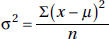
3. The variance, which is determined by averaging the squared differences of all the values from the mean
4. The standard deviation, which is the square root of the variance
EXAMPLE 2.4
The monthly rainfall in Monrovia, Liberia, where May through October is the rainy season and November through April the dry season, is as follows:
| Month: | Jan | Feb | Mar | Apr | May | June | July | Aug | Sept | Oct | Nov | Dec | |
| Rain (in.): | 1 | 2 | 4 | 6 | 18 | 37 | 31 | 16 | 28 | 24 | 9 | 4 |
The mean is

What are the measures of variability?
Answer: Range: The maximum is 37 inches (June), and the minimum is 1 inch (January). Thus the range is 37 – 1 = 36 inches of rain.
Interquartile range: Removing the lower and upper quarters leaves 4, 6, 9, 16, 18, and 24. Thus the interquartile range is 24 – 4 = 20. [The interquartile range is sometimes calculated as follows: The median of the lower half is  the median of the upper half is
  and the interquartile range is Q3 – Q1 = 22. When there is a large number of values in the set, the two methods give the same answer.]
Variance:

Standard deviation:  inches
Range
The simplest, most easily calculated measure of variability is the range. The difference between the largest and smallest values can be noted quickly, and the range gives some impression of the dispersion. However, it is entirely dependent on the two extreme values and is insensitive to the ones in the middle.
One use of the range is to evaluate samples with very few items. For example, some quality control techniques involve taking periodic small samples and basing further action on the range found in several such samples.
Interquartile Range
Finding the interquartile range is one method of removing the influence of extreme values on the range. It is calculated by arranging the data in numerical order, removing the upper and lower quarters of the values, and noting the range of the remaining values. That is, it is the range of the middle 50% of the values.
The numerical rule for designating outliers is to calculate 1.5 times the interquartile range (IQR) and then call a value an outlier if it is more than 1.5 × IQR below the first quartile or 1.5 × IQR above the third quartile.
EXAMPLE 2.5
Suppose that the starting salaries (in $1000) for college graduates who took AP Statistics in high school and at least one additional statistics class in college have the following characteristics: the smallest value is 18.8, 10% of the values are below 25.6, 25% are below 41.1, the median is 59.3, 60% are below 84.3, 75% are below 101.9, 90% are below 118.0, and the top value is 201.7.
a. What is the range?
Answer: The range is 201.7 – 18.8 = 182.9 (thousand dollars) = $182,900.
b. What is the interquartile range?
Answer: The interquartile range, that is, the range of the middle 50% of the values, is Q3 – Q1 = 101.9 – 41.1 = 60.8 (thousand dollars) = $60,800.
c. When the numerical rule is used for outliers, should either the smallest or largest value be called an outlier?
Answer: 1.5 × IQR = 1.5 × 60.8 = 91.2. If a value is more than 91.2 below the first quartile, 41.1, or more than 91.2 above the third quartile, 101.9, then it will be called an outlier. Since the largest value, 201.7, is greater than 101.9 + 91.2 = 193.1, it is considered an outlier by the given numerical rule.
Variance
Dispersion is often the result of various chance happenings. For example, consider the motion of microscopic particles suspended in a liquid. The unpredictable motion of any particle is the result of many small movements in various directions caused by random bumps from other particles. If we average the total displacements of all the particles from their starting points, the result will not increase in direct proportion to time. If, however, we average the squares of the total displacements of all the particles, this result will increase in direct proportion to time.
The same holds true for the movement of paramecia. Their seemingly random motions as seen under a microscope can be described by the observation that the average of the squares of the displacements from their starting points is directly proportional to time. Also, consider ping-pong balls dropped straight down from a high tower and subjected to chance buffeting in the air. We can measure the deviations from a center spot on the ground to the spots where the balls actually strike. As the height of the tower is increased, the average of the squared deviations increases proportionately.
In a wide variety of cases we are in effect trying to measure dispersion from the mean due to a multitude of chance effects. The proper tool in these cases is the average of the squared deviations from the mean; it is called the variance and is denoted by  2 ( is the lowercase Greek letter sigma):
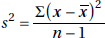
For circumstances specified later, the variance of a sample, denoted by s2, is calculated as
TIP
Most calculators give the standard deviation, and this must be squared to find the variance.
EXAMPLE 2.6
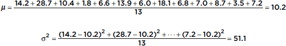
The Points Per Game (PPG) during the 2012–2013 season of the New York Knicks players were {14.2, 28.7, 10.4, 1.8, 6.6, 13.9, 6.0, 18.1, 6.8, 7.0, 8.7, 3.5, 7.2}. What was the variance?
Answer: The variance can be quickly found on any calculator with a simple statistical package, or it can be found as follows:
Standard Deviation
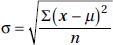
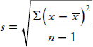
Suppose we wish to pick a representative value for the variability of a certain population. The preceding discussions indicate that a natural choice is the value whose square is the average of the squared deviations from the mean. Thus we are led to consider the square root of the variance. This value is called the standard deviation, is denoted by , and is calculated on your calculator or as follows:
Similarly, the standard deviation of a sample is denoted by s and is calculated on your calculator or as follows:
While variance is measured in square units, standard deviation is measured in the same units as are the data.
For the various x-values, the deviations x – x are called residuals, and s is a “typical value” for the residuals. While s is not the average of the residuals (the average of the residuals is always 0), s does give a measure of the spread of the x-values around the sample mean.
EXAMPLE 2.7
The number of calories in 12-ounce servings of five popular beers are {95, 152, 188, 205, 131}. Using the TI-84, 1-Var Stats gives
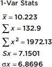
Since these data represent a sample of beers, the standard deviation is 7.1501.
MEASURING POSITION: SIMPLE RANKING, PERCENTILE RANKING, AND Z-SCORE
We have seen several ways of choosing a value to represent the center of a distribution. We also need to be able to talk about the position of any other values. In some situations, such as wine tasting, simple rankings are of interest. Other cases, for example, evaluating college applications, may involve positioning according to percentile rankings. There are also situations in which position can be specified by making use of measurements of both central tendency and variability.
There are three important, recognized procedures for designating position:
1. Simple ranking, which involves arranging the elements in some order and noting where in that order a particular value falls
2. Percentile ranking, which indicates what percentage of all values fall below the value under consideration
3. The z-score, which states very specifically by how many standard deviations a particular value varies from the mean.
EXAMPLE 2.8
It is recommended that the “good cholesterol,” high-density lipoprotein (HDL), be present in the blood at levels of at least 40 mg/dl. Suppose a 50-member high school football team are all tested with resulting HDL levels of {53, 26, 45, 33, 64, 29, 73, 29, 21, 58, 70, 41, 48, 55, 55, 39, 57, 48, 9, 59, 56, 39, 68, 50, 65, 30, 38, 54, 49, 35, 56, 70, 43, 86, 52, 40, 28, 40, 67, 50, 47, 54, 59, 29, 29, 42, 45, 37, 51, 40}. What is the position of the HDL score of 41?
Answer: Since there are 31 higher HDL levels on the list, the 41 has a simple ranking of 32 out of 50. Eighteen HDL levels are lower, so the percentile ranking is 18/50 = 36%. The above list has a mean of 47.22 with a standard deviation of 15.05, so the HDL score of 41 has a z-score of (41 – 47.22)/15.05 = –0.413.
Simple Ranking
Simple ranking is easily calculated and easily understood. We know what it means for someone to graduate second in a class of 435, or for a player from a team of size 30 to have the seventh-best batting average. Simple ranking is useful even when no numerical values are associated with the elements. For example, detergents can be ranked according to relative cleansing ability without any numerical measurements of strength.
Percentile Ranking
Percentile ranking, another readily understood measurement of position, is helpful in comparing positions with different bases. We can more easily compare a rank of 176 out of 704 with a rank of 187 out of 935 by noting that the first has a rank of 75%, and the second, a rank of 80%. Percentile rank is also useful when the exact population size is not known or is irrelevant. For example, it is more meaningful to say that Jennifer scored in the 90th percentile on a national exam rather than trying to determine her exact ranking among some large number of test takers.
The quartiles, Q1 and Q3, lie one-quarter and three-quarters of the way up a list, respectively. Their percentile ranks are 25% and 75%, respectively. The interquartile range defined earlier can also be defined to be Q3 – Q1. The deciles lie one-tenth and nine-tenths of the way up a list, respectively, and have percentile ranks of 10% and 90%.
z-Score
The z-score is a measure of position that takes into account both the center and the dispersion of the distribution. More specifically, the z-score of a value tells how many standard deviations the value is from the mean. Mathematically, x – µ gives the raw distance from µ to x; dividing by converts this to number of standard deviations. Thus  , where x is the raw score, µ is the mean, and is the standard deviation. If the score x is greater than the mean µ, then z is positive; if x is less than µ, then z is negative.
Given a z-score, we can reverse the procedure and find the corresponding raw score. Solving for x gives x = µ + z.
EXAMPLE 2.9
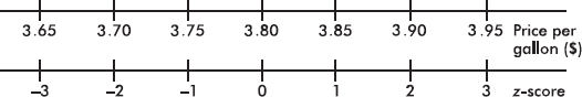
Suppose the average (mean) price of gasoline in a large city is $3.80 per gallon with a standard deviation of $0.05. Then $3.90 has a z-score of 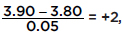 while $3.65 has a z-score of
 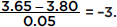 Alternatively, a z-score of +2.2 corresponds to a raw score of 3.80 + 2.2(0.05) = 3.80 + 0.11 = 3.91, while a z-score of –1.6 corresponds to 3.80 – 1.6(0.05) = 3.72.
It is often useful to portray integer z-scores and the corresponding raw scores as follows:
EXAMPLE 2.10
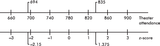
Suppose the attendance at a movie theater averages 780 with a standard deviation of 40. Adding multiples of 40 to and subtracting multiples of 40 from the mean 780 gives
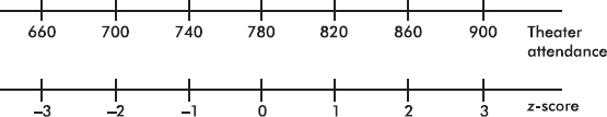
A theater attendance of 835 is converted to a z-score as follows: 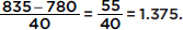
A z-score of –2.15 is converted to a theater attendance as follows: 780 – 2.15(40) = 694.
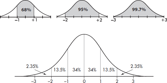
The empirical rule (also called the 68-95-99.7 rule) applies specifically to symmetric bell-shaped data (not to skewed data!). In this case, about 68% of the values lie within 1 standard deviation of the mean, about 95% of the values lie within 2 standard deviations of the mean, and more than 99% of the values lie within 3 standard deviations of the mean.
In the following figure the horizontal axis shows z-scores:
EXAMPLE 2.11
Suppose that taxicabs in New York City are driven an average of 75,000 miles per year with a standard deviation of 12,000 miles. What information does the empirical rule give us?
Answer: Assuming that the distribution is bell-shaped, we can conclude that approximately 68% of the taxis are driven between 63,000 and 87,000 miles per year, approximately 95% are driven between 51,000 and 99,000 miles, and virtually all are driven between 39,000 and 111,000 miles.
The empirical rule also gives a useful quick estimate of the standard deviation in terms of the range. We can see in the figure above that 95% of the data fall within a span of 4 standard deviations (from –2 to +2 on the z-score line) and 99.7% of the data fall within 6 standard deviations (from –3 to +3 on the z-score line). It is therefore reasonable to conclude that for these data the standard deviation is roughly between one-fourth and one-sixth of the range. Since we can find the range of a set almost immediately, the empirical rule technique for estimating the standard deviation is often helpful in pointing out gross arithmetic errors.
EXAMPLE 2.12
If the range of a bell-shaped data set is 60, what is an estimate for the standard deviation?
Answer: By the empirical rule, the standard deviation is expected to be between 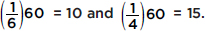 If the standard deviation is calculated to be 0.32 or 87, there is probably an arithmetic error; a calculation of 12, however, is reasonable.
However, it must be stressed that the above use of the range is not intended to provide an accurate value for the standard deviation. It is simply a tool for pointing out unreasonable answers rather than, for example, blindly accepting computer outputs.
HISTOGRAMS AND MEASURES OF CENTRAL TENDENCY
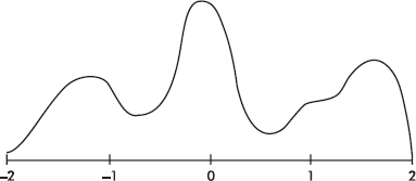
Suppose we have a detailed histogram such as
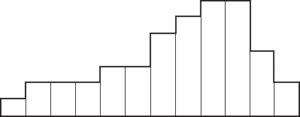
Our measures of central tendency fit naturally into such a diagram.
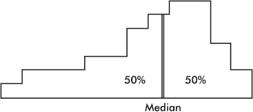
The median divides a distribution in half, so it is represented by a line that divides the area of the histogram in half.
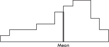
The mean is affected by the spacing of all the values. Therefore, if the histogram is considered to be a solid region, the mean corresponds to a line passing through the center of gravity, or balance point.
The above distribution, spread thinly far to the low side, is said to be skewed to the left. Note that in this case the mean is usually less than the median. Similarly, a distribution spread far to the high side is skewed to the right, and its mean is usually greater than its median.
EXAMPLE 2.13
Suppose that the faculty salaries at a college have a median of $82,500 and a mean of $88,700. What does this indicate about the shape of the distribution of the salaries?
Answer: The median is less than the mean, and so the salaries are probably skewed to the right. There are a few highly paid professors, with the bulk of the faculty at the lower end of the pay scale.
It should be noted that the above principle is a useful, but not hard-and-fast, rule.
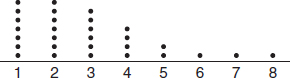
EXAMPLE 2.14
The set given by the dotplot below is skewed to the right; however, its median (3) is greater than its mean (2.97).
HISTOGRAMS, Z-SCORES, AND PERCENTILE RANKINGS
We have seen that relative frequencies are represented by relative areas, and so labeling the vertical axis is not crucial. If we know the standard deviation, the horizontal axis can be labeled in terms of z-scores. In fact, if we are given the percentile rankings of various z-scores, we can construct a histogram.
EXAMPLE 2.15
Suppose we are asked to construct a histogram from these data:
z-score: |
–2 |
–1 |
0 |
1 |
2 |
|
Percentile ranking: |
0 |
20 |
60 |
70 |
100 |
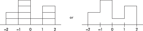
We note that the entire area is less than z-score +2 and greater than z-score –2. Also, 20% of the area is between z-scores –2 and –1, 40% is between –1 and 0, 10% is between 0 and 1, and 30% is between 1 and 2. Thus the histogram is as follows:
Now suppose we are given four in-between z-scores as well:
z-score |
Ranking |
2.0 |
100 |
1.5 |
80 |
1.0 |
70 |
0.5 |
65 |
0.0 |
60 |
–0.5 |
30 |
–1.0 |
20 |
–1.5 |
5 |
–2.0 |
0 |
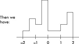
With 1000 z-scores perhaps the histogram would look like
The height at any point is meaningless; what is important is relative areas. For example, in the final diagram above, what percentage of the area is between z-scores of +1 and +2?
Answer: Still 30%.
What percent is to the left of 0?
Answer: Still 60%.
A boxplot (also called a box and whisker display) is a visual representation of dispersion that shows the smallest value, the largest value, the middle (median), the middle of the bottom half of the set (Q1), and the middle of the top half of the set (Q3).
TIP
The IQR is the length of the box, not the box itself. So the median is in the box, or is between Q1 and Q3, but is not in the IQR.
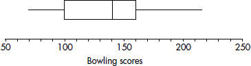
EXAMPLE 2.16
After an AP Statistics teacher hears that every one of her 27 students received a 3 or higher on the AP exam, she treats the class to a game of bowling. The individual student scores are 210, 130, 150, 140, 150, 210, 150, 125, 85, 200, 70, 150, 75, 90, 150, 115, 120, 125, 160, 140, 100, 95, 100, 215, 130, 160, and 200. Their students note that the greatest score is 215, the smallest is 70, the middle is 140, the middle of the top half is 160, and the middle of the bottom half is 100. A boxplot of these five numbers is
TIP
Be careful about describing the shape of a distribution when all that one has is a boxplot. For example, “approximately normal” is never a possible conclusion.
Note that the display consists of two “boxes” together with two “whiskers”—hence the alternative name. The boxes show the spread of the two middle quarters; the whiskers show the spread of the two outer quarters. This relatively simple display conveys information not immediately available from histograms or stem and leaf displays.
Putting the above data into a list, for example, L1, on the TI-84, not only gives the five-number summary
1-Var Stats
minX=70
Q1=100
Med=140
Q3=160
MaxX=215
TIP
Note that a boxplot gives one measure of center (the median) and two measures of variability (the range and the IQR).
but also gives the boxplot itself using STAT PLOT, choosing the boxplot from among the six type choices, and then using ZoomStat or in WINDOW letting Xmin=0 and Xmax=225.
On the TI-Nspire the data can be put in a list (here called index), and then a simultaneous multiple view is possible.
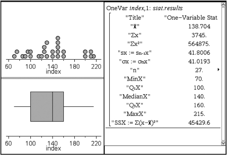
When a distribution is strongly skewed, or when it has pronounced outliers, drawing a boxplot with its five-number summary including median, quartiles, and extremes, gives a more useful description than calculating a mean and a standard deviation.
Usually, values more than 1.5 × IQR (1.5 times the interquartile range) outside the two boxes are plotted separately as outliers. (The TI-84 has a modified boxplot option. Note the two options in the second row of Type in StatPlot.)
EXAMPLE 2.17
Inputting the lengths of words in a selection of Shakespeare’s plays results in a calculator output of
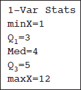
Outliers consist of any word lengths less than Q1 – 1.5(IQR) = 3 – 1.5(5 – 3) = 0 or greater than Q3 + 1.5(IQR) = 5 + 1.5(5 – 3) = 8. A boxplot indicating outliers, together with a histogram (on the TI-84 up to three different graphs can be shown simultaneously) is
Note: Some computer output shows two levels of outliers—mild (between 1.5 IQR and 3 IQR) and extreme (more than 3 IQR). In this example, the word length of 12 would be considered an extreme outlier since it is greater than 5 + 3(5 – 3) = 11.
It should be noted that two sets can have the same five-number summary and thus the same boxplots but have dramatically different distributions.
EXAMPLE 2.18
Let A = {0, 5, 10, 15, 25, 30, 35, 40, 45, 50, 71, 72, 73, 74, 75, 76, 77, 78, 100} and B = {0, 22, 23, 24, 25, 26, 27, 28, 29, 50, 55, 60, 65, 70, 75, 85, 90, 95, 100}. Simple inspection indicates very different distributions, however the TI-84 gives identical boxplots with Min = 0, Q1 = 25, Med = 50, Q3 = 75, and Max = 100 for each.
Changing units, for example, from dollars to rubles or from miles to kilometers, is common in a world that seems to become smaller all the time. It is instructive to note how measures of center and spread are affected by such changes.
Adding the same constant to every value increases the mean and median by that same constant; however, the distances between the increased values stay the same, and so the range and standard deviation are unchanged.
EXAMPLE 2.19
A set of experimental measurements of the freezing point of an unknown liquid yield a mean of 25.32 degrees Celsius with a standard deviation of 1.47 degrees Celsius. If all the measurements are converted to the Kelvin scale, what are the new mean and standard deviation?
Answer: Kelvins are equivalent to degrees Celsius plus 273.16. The new mean is thus 25.32 + 273.16 = 298.48 kelvins. However, the standard deviation remains numerically the same, 1.47 kelvins. Graphically, you should picture the whole distribution moving over by the constant 273.16; the mean moves, but the standard deviation (which measures spread) doesn’t change.
Multiplying every value by the same constant multiplies the mean, median, range, and standard deviation all by that constant.
EXAMPLE 2.20
Measurements of the sizes of farms in an upstate New York county yield a mean of 59.2 hectares with a standard deviation of 11.2 hectares. If all the measurements are converted from hectares (metric system) to acres (one acre was originally the area a yoke of oxen could plow in one day), what are the new mean and standard deviation?
Answer: One hectare is equivalent to 2.471 acres. The new mean is thus 2.471 × 59.2 = 146.3 acres with a standard deviation of 2.471 × 11.2 = 27.7 acres. Graphically, multiplying each value by the constant 2.471 both moves and spreads out the distribution.
SUMMARY
 The two principle measurements of the center of a distribution are the mean and the median.
The principle measurements of the spread of a distribution are the range (maximum value minus minimum value), the interquartile range (IQR = Q3 – Q1), the variance, and the standard deviation.
Adding the same constant to every value in a set adds the same constant to the mean and median but leaves all the above measures of spread unchanged.
Multiplying every value in a set by the same constant multiplies the mean, median, range, IQR, and standard deviation by that constant.
The mean, range, variance, and standard deviation are sensitive to extreme values, while the median and interquartile range are not.
The principle measurements of position are simple ranking, percentile ranking, and the z-score (which measures the number of standard deviations from the mean).
The empirical rule (the 68-95-99.7 rule) applies specifically to symmetric bell-shaped data.
In skewed left data, the mean is usually less than the median, while in skewed right data, the mean is usually greater than the median.
Boxplots visually show the five-number summary: the minimum value, the first quartile (Q1), the median, the third quartile (Q3), and the maximum value; and usually indicate outliers as distinct points.
Note that two sets can have the same five-number summary and thus the same boxplots but have dramatically different distributions.
QUESTIONS ON TOPIC TWO: SUMMARIZING DISTRIBUTIONS
Multiple-Choice Questions
Directions: The questions or incomplete statements that follow are each followed by five suggested answers or completions. Choose the response that best answers the question or completes the statement.
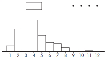
1. The graph below shows household income in Laguna Woods, California.
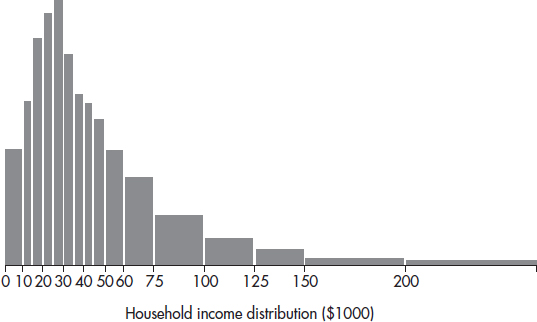
What can be said about the ratio 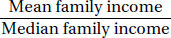 ?
?
(A) Approximately zero
(B) Less than one, but definitely above zero
(C) Approximately one
(D) Greater than one
(E) Cannot be answered without knowing the standard deviation
2. Which of the following are true statements?
I. The range of the sample data set is never greater than the range of the population.
II. The interquartile range is half the distance between the first quartile and the third quartile.
III. While the range is affected by outliers, the interquartile range is not.
(A) I only
(B) II only
(C) III only
(D) I and II
(E) I and III
3. Dieticians are concerned about sugar consumption in teenagers’ diets (a 12-ounce can of soft drink typically has 10 teaspoons of sugar). In a random sample of 55 students, the number of teaspoons of sugar consumed for each student on a randomly selected day is tabulated. Summary statistics are noted below:
Min = 10 Max = 60 First quartile = 25 Third quartile = 38
Median = 31 Mean = 31.4 n = 55 s = 11.6
Which of the following is a true statement?
(A) None of the values are outliers.
(B) The value 10 is an outlier, and there can be no others.
(C) The value 60 is an outlier, and there can be no others.
(D) Both 10 and 60 are outliers, and there may be others.
(E) The value 60 is an outlier, and there may be others at the high end of the data set.
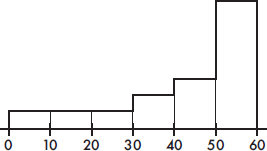
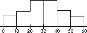
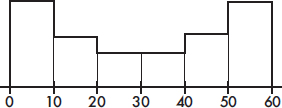
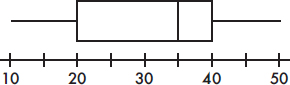
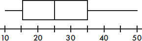
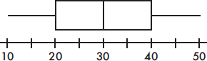
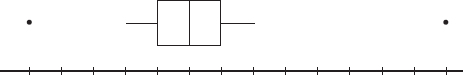
Problems 4–6 refer to the following five boxplots.
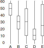
4. To which of the above boxplots does the following histogram correspond?
(A) A
(B) B
(C) C
(D) D
(E) E
5. To which of the above boxplots does the following histogram correspond?
(A) A
(B) B
(C) C
(D) D
(E) E
6. To which of the above boxplots does the following histogram correspond?
(A) A
(B) B
(C) C
(D) D
(E) E
Problems 7–9 refer to the following five histograms:
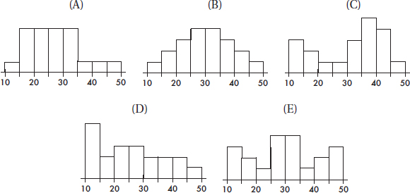
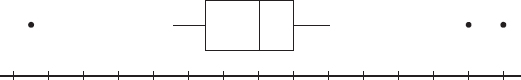
7. To which of the above histograms does the following boxplot correspond?
(A) A
(B) B
(C) C
(D) D
(E) E
8. To which of the above histograms does the following boxplot correspond?
(A) A
(B) B
(C) C
(D) D
(E) E
9. To which of the above histograms does the following boxplot correspond?
(A) A
(B) B
(C) C
(D) D
(E) E
10. Below is a boxplot of CO2 levels (in grams per kilometer) for a sampling of 2008 vehicles.
Suppose follow-up testing determines that the low outlier should be 10 grams per kilometer less and the two high outliers should each be 5 grams per kilometer greater. What effect, if any, will these changes have on the mean and median CO2 levels?
(A) Both the mean and median will be unchanged.
(B) The median will be unchanged, but the mean will increase.
(C) The median will be unchanged, but the mean will decrease.
(D) The mean will be unchanged, but the median will increase.
(E) Both the mean and median will change.
11. Below is a boxplot of yearly tuition and fees of all four year colleges and universities in a Western state. The low outlier is from a private university that gives full scholarships to all accepted students, while the high outlier is from a private college catering to the very rich.
Removing both outliers will effect what changes, if any, on the mean and median costs for this state’s four year institutions of higher learning?
(A) Both the mean and the median will be unchanged.
(B) The median will be unchanged, but the mean will increase.
(C) The median will be unchanged, but the mean will decrease.
(D) The mean will be unchanged, but the median will increase.
(E) Both the mean and median will change.
12. Suppose the average score on a national test is 500 with a standard deviation of 100. If each score is increased by 25, what are the new mean and standard deviation?
(A) 500, 100
(B) 500, 125
(C) 525, 100
(D) 525, 105
(E) 525, 125
13. Suppose the average score on a national test is 500 with a standard deviation of 100. If each score is increased by 25%, what are the new mean and standard deviation?
(A) 500, 100
(B) 525, 100
(C) 625, 100
(D) 625, 105
(E) 625, 125
14. If quartiles Q1 = 20 and Q3 = 30, which of the following must be true?
I. The median is 25.
II. The mean is between 20 and 30.
III. The standard deviation is at most 10.
(A) I only
(B) II only
(C) III only
(D) All are true.
(E) None are true.
15. A 1995 poll by the Program for International Policy asked respondents what percentage of the U.S. budget they thought went to foreign aid. The mean response was 18%, and the median was 15%. (The actual amount is less than 1%.) What do these responses indicate about the likely shape of the distribution of all the responses?
(A) The distribution is skewed to the left.
(B) The distribution is skewed to the right.
(C) The distribution is symmetric around 16.5%.
(D) The distribution is bell-shaped with a standard deviation of 3%.
(E) The distribution is uniform between 15% and 18%.
16. Assuming that batting averages have a bell-shaped distribution, arrange in ascending order:
I. An average with a z-score of –1.
II. An average with a percentile rank of 20%.
III. An average at the first quartile, Q1.
(A) I, II, III
(B) III, I, II
(C) II, I, III
(D) II, III, I
(E) III, II, I
17. Which of the following are true statements?
I. If the sample has variance zero, the variance of the population is also zero.
II. If the population has variance zero, the variance of the sample is also zero.
III. If the sample has variance zero, the sample mean and the sample median are equal.
(A) I and II
(B) I and III
(C) II and III
(D) I, II, and III
(E) None of the above gives the complete set of true responses.
18. When there are multiple gaps and clusters, which of the following is the best choice to give an overall picture of a distribution?
(A) Mean and standard deviation
(B) Median and interquartile range
(C) Boxplot with its five-number summary
(D) Stemplot or histogram
(E) None of the above are really helpful in showing gaps and clusters.
19. Suppose the starting salaries of a graduating class are as follows:
|
Number of Students |
Starting Salary ($) |
|
10 |
15,000 |
|
17 |
20,000 |
|
25 |
25,000 |
|
38 |
30,000 |
|
27 |
35,000 |
|
21 |
40,000 |
|
12 |
45,000 |
What is the mean starting salary?
(A) $30,000
(B) $30,533
(C) $32,500
(D) $32,533
(E) $35,000
20. When a set of data has suspect outliers, which of the following are preferred measures of central tendency and of variability?
(A) mean and standard deviation
(B) mean and variance
(C) mean and range
(D) median and range
(E) median and interquartile range
21. If the standard deviation of a set of observations is 0, you can conclude
(A) that there is no relationship between the observations.
(B) that the average value is 0.
(C) that all observations are the same value.
(D) that a mistake in arithmetic has been made.
(E) none of the above.
22. A teacher is teaching two AP Statistics classes. On the final exam, the 20 students in the first class averaged 92 while the 25 students in the second class averaged only 83. If the teacher combines the classes, what will the average final exam score be?
(A) 87
(B) 87.5
(C) 88
(D) None of the above
(E) More information is needed to make this calculation.
23. Suppose 10% of a data set lie between 40 and 60. If 5 is first added to each value in the set and then each result is doubled, which of the following is true?
(A) 10% of the resulting data will lie between 85 and 125.
(B) 10% of the resulting data will lie between 90 and 130.
(C) 15% of the resulting data will lie between 80 and 120.
(D) 20% of the resulting data will lie between 45 and 65.
(E) 30% of the resulting data will lie between 85 and 125.
24. The 70 highest dams in the world have an average height of 206 meters with a standard deviation of 35 meters. The Hoover and Grand Coulee dams have heights of 221 and 168 meters, respectively. The Russian dams, the Nurek and Charvak, have heights with z-scores of +2.69 and –1.13, respectively. List the dams in order of ascending size.
(A) Charvak, Grand Coulee, Hoover, Nurek
(B) Charvak, Grand Coulee, Nurek, Hoover
(C) Grand Coulee, Charvak, Hoover, Nurek
(D) Grand Coulee, Charvak, Nurek, Hoover
(E) Grand Coulee, Hoover, Charvak, Nurek
25. The first 115 Kentucky Derby winners by color of horse were as follows: roan, 1; gray, 4; chestnut, 36; bay, 53; dark bay, 17; and black, 4. (You should “bet on the bay!”) Which of the following visual displays is most appropriate?
(A) Bar chart
(B) Histogram
(C) Stemplot
(D) Boxplot
(E) Time plot
For Questions 26 and 27 consider the following: The graph below shows cumulative proportions plotted against grade point averages for a large public high school.
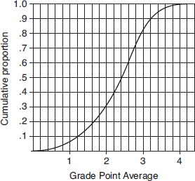
26. What is the median grade point average?
(A) 0.8
(B) 2.0
(C) 2.4
(D) 2.5
(E) 2.6
27. What is the interquartile range?
(A) 1.0
(B) 1.8
(C) 2.4
(D) 2.8
(E) 4.0
28. The following dotplot shows the speeds (in mph) of 100 fastballs thrown by a major league pitcher.
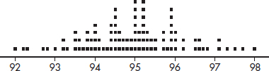
Which of the following is the best estimate of the standard deviation of these speeds?
(A) 0.5 mph
(B) 1.1 mph
(C) 1.6 mph
(D) 2.2 mph
(E) 6.0 mph
FREE-REPONSE QUESTIONS
Directions: You must show all work and indicate the methods you use. You will be graded on the correctness of your methods and on the accuracy of your final answers.
FOUR OPEN-ENDED QUESTIONS
1. Victims spend from 5 to 5840 hours repairing the damage caused by identity theft with a mean of 330 hours and a standard deviation of 245 hours.
(a) What would be the mean, range, standard deviation, and variance for hours spent repairing the damage caused by identity theft if each of the victims spent an additional 10 hours?
(b) What would be the mean, range, standard deviation, and variance for hours spent repairing the damage caused by identity theft if each of the victims’ hours spent increased by 10%?
2. In a study of all school districts in a state, the median 4-year graduation rate was 78.0% with Q1 = 60.4% and Q3 = 82.6%. The only rates below Q1 or above Q3 were 26.4%, 32.2%, 49.0%, 57.9%, 88.3%, and 98.1%.
(a) Draw a boxplot.
(b) Describe the distribution.
(c) Is the mean 4-year graduation rate probably close to, below, or above 78.0%? Explain.
(d) Would a stemplot give more, less, or basically the same information?
3. The Children’s Health Insurance Program (CHIP) provides health benefits to children from families whose incomes exceed the eligibility for Medicaid. Each state sets its own eligibility criteria. The following boxplot shows recent yearly expenditures on this program by state.
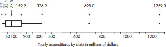
(a) What are the median and interquartile range of the distribution of yearly state expenditures in the CHIP program?
(b) Suppose the federal government takes over three million dollars of administrative costs from the state CHIP expenditures. What are the median and interquartile range of the new reduced expenditure distribution?
(c) Suppose instead the federal government picks up the tab for half of all state CHIP expenditures. What are the median and interquartile range of this new reduced expenditure distribution?
(d) Based on the above boxplot, which of the following is the most reasonable value for the mean state expenditure (in millions of dollars): 78, 135, 325, 630, or 750? Explain.
4. Suppose a distribution has mean 300 and standard deviation 25. If the z-score of Q1 is –0.7 and the z-score of Q3 is 0.7, what values would be considered to be outliers?
5. (a) Draw the boxplot for the data set {0, 1, 2, 3, 4, 5, 6, 7, 8, 9, 10}. Very different sets can have the same boxplot.
(b) Find the data set with sample size n = 11, with each value an integer between 0 and 10, and with the same boxplot as in (a), which has the smallest possible mean.
(c) Find the data set with sample size n = 11, with each value an integer between 0 and 10, and with the same boxplot as in (a), which has the largest possible standard deviation.
AN INVESTIGATIVE TASK
A measure of variability is the median absolute deviation (MAD) defined as the median deviation from the median, that is, as the median of the absolute values of the deviations from the median. For example, the median of {1, 3, 7, 10, 11, 12} is 8.5, the absolute deviations from the median are {7.5, 5.5, 1.5, 1.5, 2.5, 3.5}, and the median of these deviations, MAD, is (2.5 + 3.5)/2 = 3.
The 12 students in an AP Statistics class all score above 33 (the cutoff score that year for achieving a 3 or above): {35, 38, 38, 42, 44, 48, 50, 52, 56, 60, 62, 71}.
(a) Calculate the median of these data.
(b) Calculate the MAD for these data. Show your work.
(c) Show that half of these data values are closer than one MAD to the median and half are further than one MAD from the median.
(d) How would the calculation of MAD have changed if the top score was 76 rather than 71? Justify your answer.
(e) What does the answer to (d) say about one difference between the two measures of variability: MAD versus standard deviation?