Chapter 10
The Ratio and Reciprocal Functions
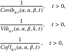
Our attention to this point has largely been focused on the primary fractional trigonometric functions, that is, the generalizations of the sine and cosine functions. In this chapter, we expand our considerations to include their reciprocals and ratios. When both the complexity and the parity functions are considered, there are a total of 36 new functions defined. We limit the consideration to the principal, k = 0, meta-trigonometric functions. From the previous chapter, they are, for t > 0:

10.1 Fractional Complexity Functions
The naming convention for the complexity fractional meta-trigonometric functions will follow that for the integer-order trigonometry; thus, we have


To minimize the number of plots, the graphic displays for the complexity functions are based on the natural quency simplification forms of equations (E.21) and (E.22). Figures 10.1–10.6 show the effect of variations in q for the fractional complexity meta-trigonometric functions for  ,
,  ,
,  , q = 0.25–1.5 in steps of 0.25, t = 0–10.

Figure 10.1 Effect of q with;  versus t-Time for
  ,
,  ,
,  , and q = 0.25–1.5 in steps of 0.25, t = 0–10.

Figure 10.2 Effect of q with;  versus t-Time for
  ,
,  ,
,  , and q = 0.25–1.5 in steps of 0.25, t = 0–10.

Figure 10.3 Effect of q with;  versus t-Time for
  ,
,  ,
,  , and q = 0.25–1.5 in steps of 0.25, t = 0–10.

Figure 10.4 Effect of q with;  versus t-Time for
  ,
,  ,
,  , and q = 0.25–1.5 in steps of 0.25, t = 0–10.

Figure 10.5 Effect of q with;  versus t-Time for
  ,
,  ,
,  , and q = 0.25–1.5 in steps of 0.25, t = 0–10.

Figure 10.6 Effect of q with;  versus t-Time for
  ,
,  ,
,  , and q = 0.25–1.5 in steps of 0.25, t = 0–10.
10.2 The Parity Reciprocal Functions
The parity reciprocal functions are listed as

and

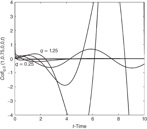
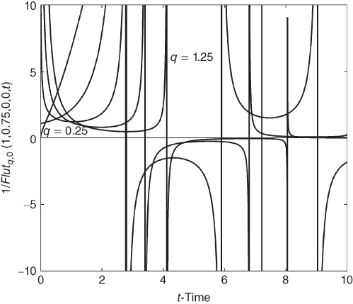
when they exist. Figures 10.7–10.14 show the effect of variations in q for each of the parity meta-trigonometric functions and their reciprocals with  , a = 1.0,
  , q = 0.25–1.25 in steps of 0.25, t = 0–10.

Figure 10.7 Effect of q with  versus t-Time for
  ,
,  , a = 1.0,
  , q = 0.25–1.25 in steps of 0.25, t = 0–10.

Figure 10.8 Effect of q with  versus t-Time for
  ,
,  , a = 1.0,
  , q = 0.25–1.25 in steps of 0.25, t = 0–10.

Figure 10.9 Effect of q with  versus t-Time for
  ,
,  , a = 1.0,
  , q = 0.25–1.25 in steps of 0.25, t = 0–10.

Figure 10.10 Effect of q with  versus t-Time for
  ,
,  , a = 1.0,
  , q = 0.25–1.25 in steps of 0.25, t = 0–10.

Figure 10.11 Effect of q with  versus t-Time for
  ,
,  , a = 1.0,
  , q = 0.25–1.25 in steps of 0.25, t = 0–10.

Figure 10.12 Effect of q with 1/ versus t-Time for
  ,
,  , a = 1.0,
  , q = 0.25–1.25 in steps of 0.25, t = 0–10.

Figure 10.13 Effect of q with  versus t-Time for
  ,
,  , a = 1.0,
  , q = 0.25–1.25 in steps of 0.25, t = 0–10.

Figure 10.14 Effect of q with 1/ versus t-Time for
  ,
, , a = 1.0,
  , q = 0.25–1.25 in steps of 0.25, t = 0–10.
10.3 The Parity Ratio Functions
We consider only 2 of the 36 possible ratio functions for the parity meta-trigonometric functions. They are as follows:

Figures 10.15 and 10.16 show the effect of q for these ratio functions versus t-Time for  , a = 1.0,
  , q = 0.5–1.25 in steps of 0.25, t = 0–10. The general appearance of these function is similar to that of the
  , as seen in Figure 10.3.

Figure 10.15 Effect of q with  versus t-Time for
  ,
,  , a = 1.0,
  , q = 0.5–1.25 in steps of 0.25, t = 0–10.

Figure 10.16 Effect of q with  versus t-Time for
  ,
,  , a = 1.0,
  , q = 0.5–1.25 in steps of 0.25, t = 0–10.
10.4 R-Function Representation of the Fractional Ratio and Reciprocal Functions
The R-function representations for the ratio and reciprocal functions are easily determined using the results from Section 9.5. Thus, we have for t > 0


10.5 Relationships
From equation (9.176), we have
Dividing by  gives
gives


or

This is a broad generalization of the trigonometric identity  .
.
Dividing equation (10.14) by  yields

or

This is a generalization of the identity  . Many similar identities may also be written for the parity functions.
10.6 Discussion
There is much to be done in this area and this presentation only begins to scratch the surface. Because of the many possible ratio and reciprocal functions, it is important that a simple naming convention be established that is based on the numerator and denominator functions.
The following possibility is offered. Consider the associations

Then, using lower case “r” to represent “the reciprocal of,” we have  , and so on. Furthermore,
  ,
,  , and so on for the names of the ratio functions with “o” representing “over.”
Importantly, we need to know what special properties may be associated with these functions, whether series expansions can be developed, and whether there are geometric interpretations beyond triangles that may be useful.
