Chapter 9
The Fractional Meta-Trigonometry
In the previous four chapters, fractional generalizations of the integer-order trigonometric and hyperbolic functions have been developed. In Chapters 5 and 6, we have seen the relationship of the R1-trigonometry to the R1-hyperboletry. Such a direct relationship for the R2-trigonometry, however, has not been found. After some study of this problem, it has become apparent that more complicated relationships exist between the bases for the various trigonometries. This chapter presents a generalization that helps explore these connections. Furthermore, the chapter contains the hyperboletry1 and all1 of the trigonometries that we have explored to this point. This chapter also presents new trigonometries (Lorenzo [82, 83]) not previously available and potentially allows the solution of linear fractional differential equations in terms of these special functions. The result then is the master fractional trigonometry based on the R-function.
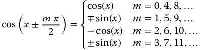
The bases of the trigonoboletries that we have considered to this point are as follows:

Clearly, trigonometries can be created for, or associated with, all of the indexed forms of the R-function presented in Table 3.2, which is a total of 16 integer-valued bases. Many of these bases will likely have important application in the fractional calculus and in the solution of fractional differential equations. However, a more global approach is considered here. This chapter considers fractional meta-trigonometries based on

With  and
and  ranging between 0 and 4, all of the integer-valued bases are considered together with infinitely more noninteger possibilities.
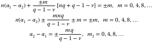
Multiplication of the a or t variables by  rotates the variable in the complex plane by the amount
  radians. This is shown graphically in Figure 9.1. These rotations can have profound effects on the real and imaginary projections, which relate to the generalized functions. This chapter is adapted from Lorenzo [82, 83], with permission of ASME.
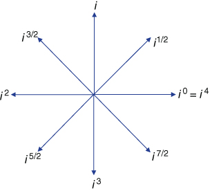
Figure 9.1 Graphical display of  for
for  in steps of
  .
.
Source: Lorenzo 2009a [82]. Reproduced with permission of ASME.
9.1 The Fractional Meta-Trigonometric Functions: Based on Complexity
We start by separating  into real and imaginary parts. Thus, we consider
Now, for rational q, v,  , and
, and  , we may write
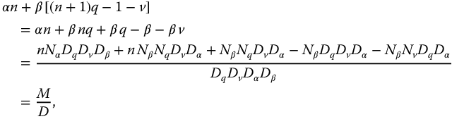
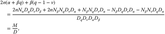
where  ,
,  ,
,  , and
, and  . Then, we may write

where  or
or  and
and  , and M/D is rational and in minimal form.
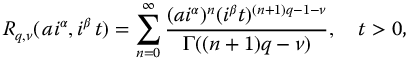
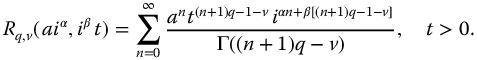
Therefore, equation (9.2) may be written as
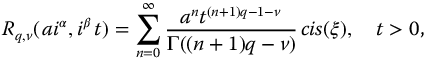
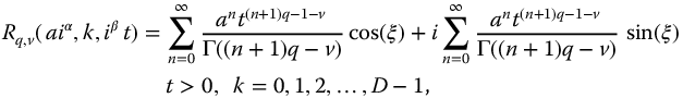
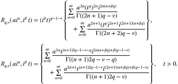
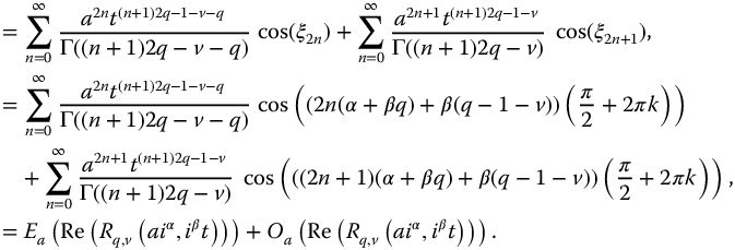
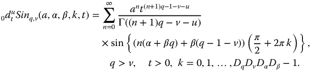
where k is included in the R-function argument to reflect its presence in  on the right-hand side. Then, similar to the earlier definitions, we define the generalized fractional functions as

These definitions generalize those for the trignoboletries that were developed in previous chapters. The notation is changed, and here drops the preceding R and its subscript. These fractional meta-trigonometric functions are discriminated from the traditional trigonometric functions by the capitalization and the subscripted order variables. Continuing from Ref. [82] with permission of ASME:
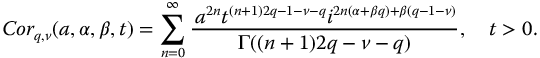
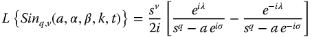
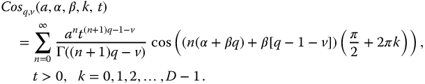
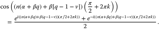
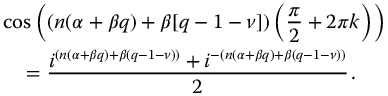
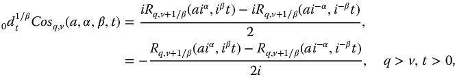
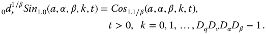
As with the previous trigonometric functions, we define the principal functions for t > 0 as

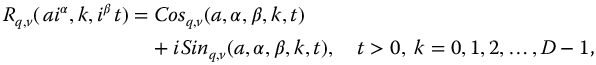
where D is the product of the denominators of  in minimal form. This is the generalized fractional Euler equation. A complimentary fractional meta-Euler equation is derived later as equation (9.173).
9.1.1 Alternate Forms
It should be noted that the form of equation (9.1) was chosen for the convenience that it allowed either the “a” and/or the “t” variables to be made complex. The cost of this convenience, however, was to introduce two new variables,  , into the defining summation. Complexly proportional forms with one less variable in the summation are possible and are discussed in Appendix E.
9.1.2 Graphical Presentation – Complexity Functions
A complete graphical presentation for the  - and
- and  -functions is, of course, impossible. There are seven parameters and variables, and the possible number of charts is limitless. In previous chapters, the effects of variations of q and v have been presented with
  and
and  values of zero and one. Therefore, the emphasis here is on the new variables introduced in this chapter, namely
  and
and  .
.
Figures 9.2–9.5 show the effect of varying  in the
  for q = 1.05, 1.00, 0.75, and 0.50, with a = 1.0,
  , and with
  variations from 1.0 to 3.0. For the
  -function in Figure 9.3, we see that
  over the range shown.
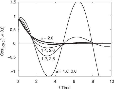
Figure 9.2 Effect of  on
on 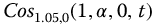 with
with  = 1.0–3.0 in steps of 0.2, with q = 1.05, a = 1,
  , v = 0, k = 0.
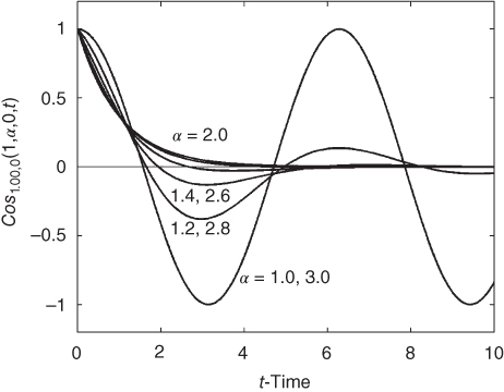
Figure 9.3 Effect of  on
on  with
with  = 1.0–3.0 in steps of 0.2, with q = 1.00, a = 1,
  , v = 0, k = 0.
Source: Lorenzo 2009a [82]. Adapted with permission of ASME.
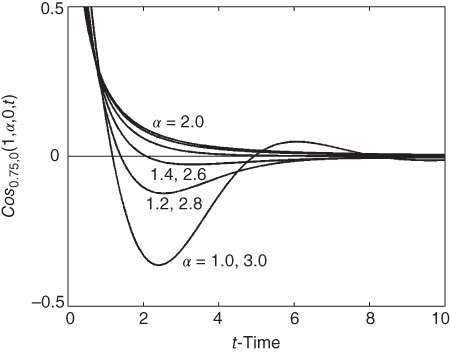
Figure 9.4 Effect of  on
on 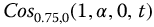 with
with  = 1.0–3.0 in steps of 0.2, with q = 0.75, a = 1,
  , v = 0, k = 0.
Figure 9.5 Effect of  on
on  with
with  = 1.0–3.0 in steps of 0.2, with q = 0.25, a = 1,
  , v = 0, k = 0.
The study is repeated for  in Figures 9.6–9.9. For the
  -functions, in these figures, it can be seen that the behavior is symmetric around
  ; that is,
  for
for 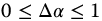 .
.
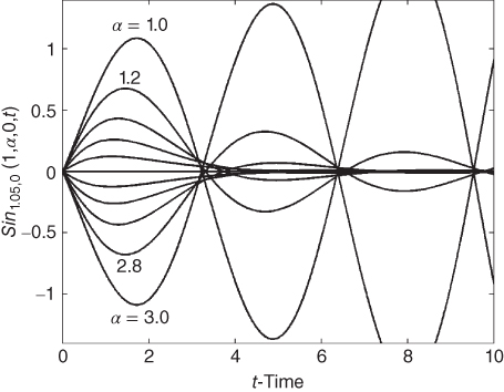
Figure 9.6 Effect of  on
on  with
with  = 1.0–3.0 in steps of 0.2, with q = 1.05, a = 1,
  , v = 0, k = 0.
Figure 9.7 Effect of  on
on  with
with  = 1.0–3.0 in steps of 0.2, with q = 1.00, a = 1,
  , v = 0, k = 0.
Source: Lorenzo 2009a [82]. Adapted with permission of ASME.
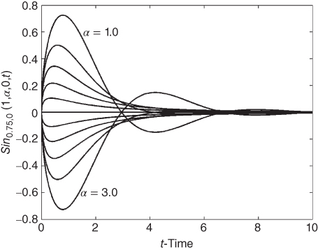
Figure 9.8 Effect of  on
on  with
with  = 1.0–3.0 in steps of 0.2, with q = 0.75, a = 1,
  , v = 0, k = 0.
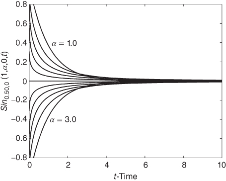
Figure 9.9 Effect of on with = 1.0–3.0 in steps of 0.2, with q = 0.50, a = 1, , v = 0, k = 0.
In Figure 9.7, the fractional trigonometric functions appear to be quite similar to exponentially damped sinusoids or cosinusoids. The common feature of these figures is the selection of variables, that is, 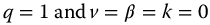 . Continuing from Ref. [84] with permission of ASME:
Relative to Figure 9.7, we have from equation (9.7)
Now, from Ref. [56], pp. 118–119, #632,

Thus,

a closed-form summation. Also, based on Ref. [56], pp. 116–117, #631, we can determine

Because
is simply a constant for any individual curve, we see that for these special cases the functions are indeed exponentially damped sinusoids under the
constraints.
The effects of variations in
on
with
= 1.0–3.0 in steps of 0.2, is shown in Figures 9.10a–9.13. Symmetry around
, similar to that observed for the
variations, is seen in Figure 9.11 for
. The effect of
variations on the fractional
-functions is presented in Figures 9.14–9.17. For values of q < 1, an increase in
increases the apparent damping as seen in Figures 9.16 and 9.17.
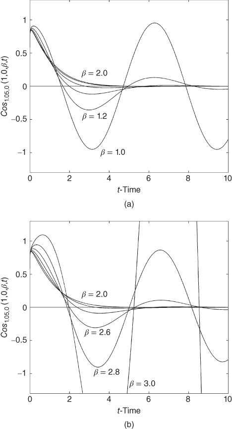
Figure 9.10 Effect of  on
on  with (a)
  = 1.0–2.0 and (b)
  = 2.0–3.0 in steps of 0.2, with q = 1.05, a = 1,
  , v = 0, k = 0.
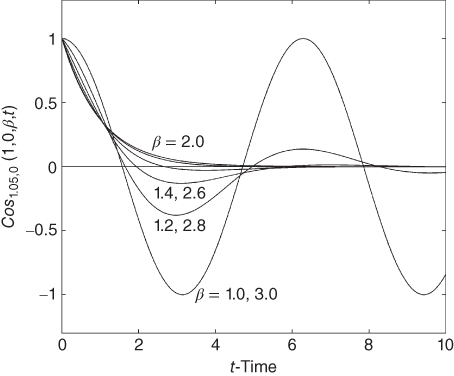
Figure 9.11 Effect of  on
on  with
with  = 1.0–3.0 in steps of 0.2, with q = 1.00, a = 1,
  , v = 0, k = 0.
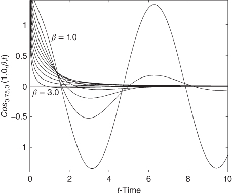
Figure 9.12 Effect of  on
on 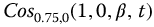 with
with  = 1.0–3.0 in steps of 0.2, with q = 0.75, a = 1,
  , v = 0, k = 0.
Figure 9.13 Effect of  on
on  with
with  = 1.0–3.0 in steps of 0.2, with q = 0.50, a = 1,
  , v = 0, k = 0.
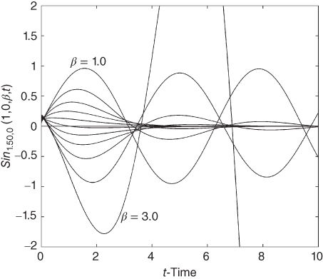
Figure 9.14 Effect of  on
on  with
with  = 1.0–3.0 in steps of 0.2, with q = 1.05, a = 1,
  , v = 0, k = 0.
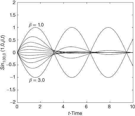
Figure 9.15 Effect of  on
on  with
with  = 1.0–3.0 in steps of 0.2, with q = 1.05, a = 1,
  , v = 0, k = 0.
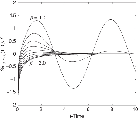
Figure 9.16 Effect of  on
on  with
with  = 1.0–3.0 in steps of 0.2, with q = 0.75, a = 1,
  , v = 0, k = 0.
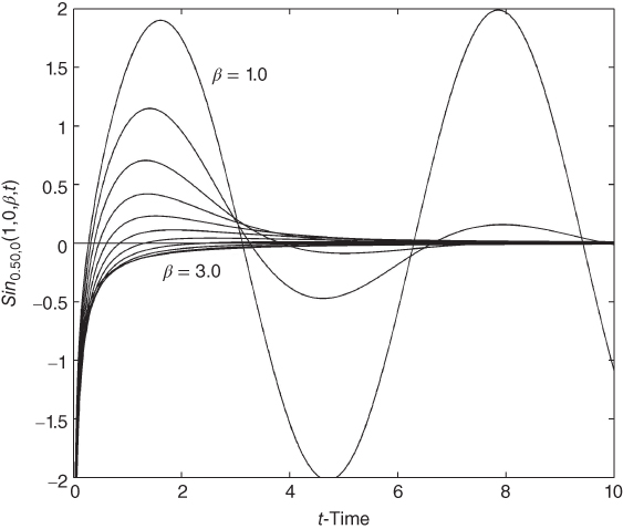
Figure 9.17 Effect of  on
on  with
with  = 1.0–3.0 in steps of 0.2, with q = 0.50, a = 1,
  , v = 0, k = 0.
Phase plane plots of Figures 9.18–9.21 study the effects of variations in  for values of q = 1.05, 1.00, 0.95, and 0.50. A significant change in the nature of these cross plots is seen with small variations of q around q = 1.0 in Figures 9.18–9.20. We notice in Figure 9.21 the loss of oscillation due to the small value of q.

Figure 9.18 Phase plane  versus
  for
for  = 1–3 in steps of 0.2, with a = 1.0, q = 1.00,
  , k = 0, v = 0. Arrows indicate increasing function.
Source: Lorenzo 2009a [82]. Adapted with permission of ASME.

Figure 9.19 Phase plane  versus
  for
for  = 1–3 in steps of 0.2, with a = 1.0, q = 1.05, k = 0,
  , v = 0. Arrows indicate increasing function parameter.
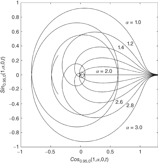
Figure 9.20 Phase plane  versus
  for
for  = 1–3 in steps of 0.2, with a = 1.0, q = 0.95, k = 0,
  , v = 0.
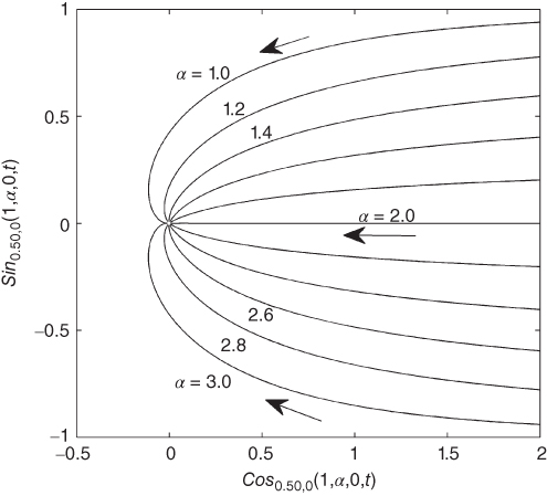
Figure 9.21 Phase plane  versus
  for
for  = 1–3 in steps of 0.2, with a = 1.0, q = 0.50, k = 0,
  , v = 0. Arrows indicate increasing function parameter.
Figures 9.22 and 9.23 show the effect of  on the phase plane behavior of
  versus
  with q = 1,
  , a = 1, and k = 0. By comparing these two figures, the effect of v,
  , is seen to have a strong effect on the function behavior.
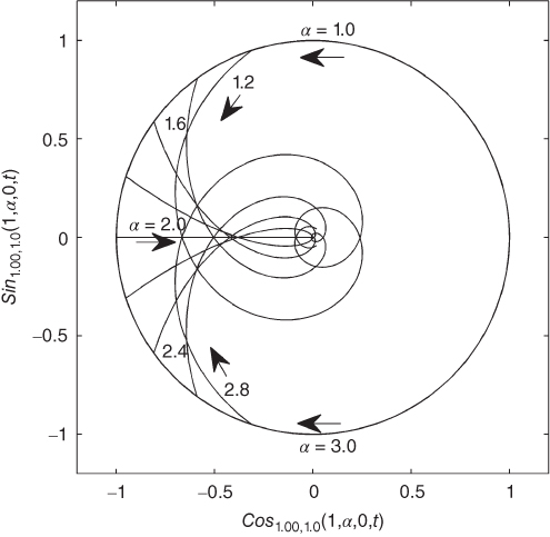
Figure 9.22 Phase plane 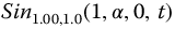 versus
  for
for  = 1–3 in steps of 0.2, with v = 1.0, a = 1.0, q = 1.00, k = 0,
  . Arrows indicate increasing function parameter.
Source: Lorenzo 2009a [82]. Adapted with permission of ASME.
Figure 9.23 Phase plane  versus
  for
for  = 1–3 in steps of 0.2, with v = −1.0, a = 1.0, q = 1.00, k = 0,
  .
.
Figures 9.24 and 9.25 show the effect of  on the fractional
  for q = 1.15 and q = 0.95. Note, for q > 1 the functions depart from the origin and for q < 1 the functions arrive from infinity. Figure 9.26 shows the phase plane,
  versus
  , for
, for  . Here, all the functions arrive from infinity with increasing t. However, for
  the functions are captured by the origin, while for
  the functions are repelled by the unit circle.
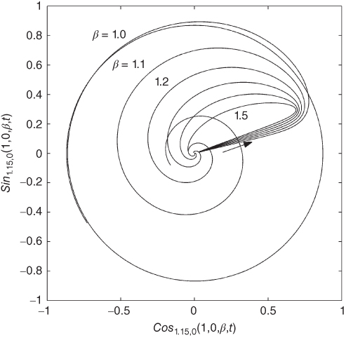
Figure 9.24 Phase plane  versus
  for
for  = 1–1.5 in steps of 0.1, with q = 1.15, v = 0, a = 1.0, k = 0,
  .
.
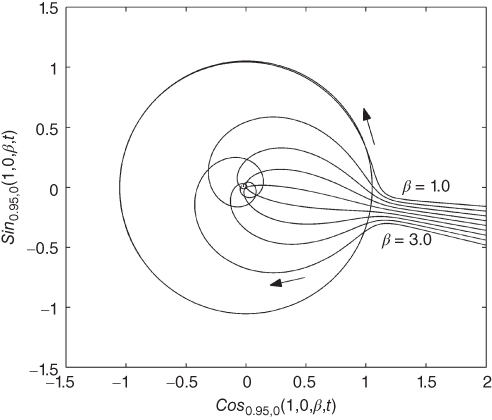
Figure 9.25 Phase plane  versus
  for
for  = 1–3 in steps of 0.25, with q = 0.95, v = 0, a = 1.0, k = 0,
  .
.
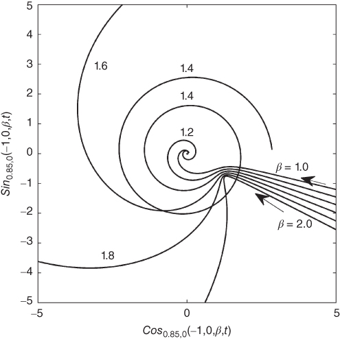
Figure 9.26 Phase plane  versus
  for
for  = 1–2 in steps of 0.2, with a = −1.0, q = 0.85, v = 0, k = 0,
  , t = 0–12.
Because of symmetrical occurrences in some physical processes, Figures 9.27–9.31 present the  - versus
  -functions together with their symmetric partners
  versus
  . Figure 9.31 shows an instance of a barred spiral. Such spirals are of interest in astrophysics; see Chapter 18. The various other special cases are self-explanatory.
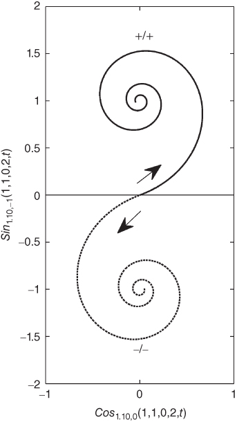
Figure 9.27 Phase plane  versus
  and
and  versus
  for
for  = 0.2, with a = 1.0, q = 1.10, v = −1, k = 0,
  , t = 0–18.
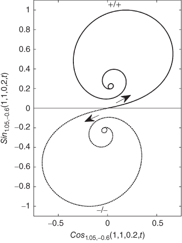
Figure 9.28 Phase plane 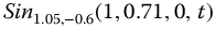 versus
  and for
  versus
  = 0, with a = 1.0, q = 1.05, v = 0.2, k = 0,
  , t = 0–20.
Figure 9.29 Phase plane  versus
  and for
  versus
  ,
,  = 0.1, with a = 1.0, q = 1.05, v = 0, k = 0,
  , t = 0–20.
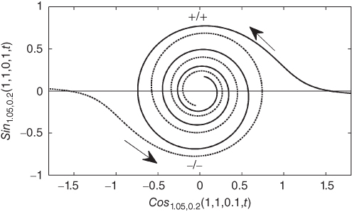
Figure 9.30 Phase plane  versus
  and for
  versus
  = 0.1, with a = 1.0, q = 1.05, v = 0.2, k = 0,
  , t = 0–20.

Figure 9.31 Phase plane  versus
  and for
  versus
  ,
,  = 0, with a = 1.0, q = 1.05, v = 0.05, k = 0,
  , t = 0–10.
9.2 The Meta-Fractional Trigonometric Functions: Based on Parity
Continuing from Ref. [82] with permission of ASME:
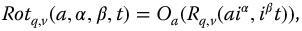
We now consider
based on parity of the exponent of a. Then, equation (9.1) is written as
The summation becomes
9.17 
Forming two summations by separating the even and odd powers of a, we have
This also may be expressed as
9.20 
The summations of equation (9.19) contain the even and odd powers of a, respectively. In parallel with the previous development of the R-trigonometric functions, we define the generalized or meta-Corotation and Rotation functions as
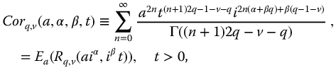

where the nomenclature  means the terms with even powers of a in
  .
.
Similarly,

and where the nomenclature  means the terms with odd powers of a in
  .
.
As in the previous trigonometries, the generalized Corotation and Rotation functions are also, in general, complex. Clearly, we may also write

The real and imaginary parts of these functions are now used to define the four new real fractional meta-trigonometric functions. The
-function is given in equation (9.21) as
Now, applying equation (3.123) to
with
rational, we have
with M/D a rational number in minimal form. Thus, the  may be written as

where  . The real part of the
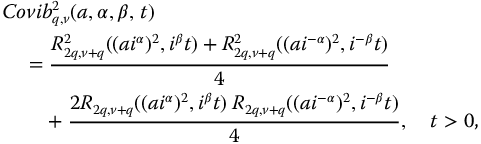
  is now defined as the generalized or meta-Covibration function
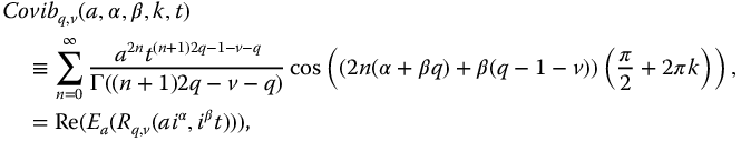
with t > 0, and  .
.
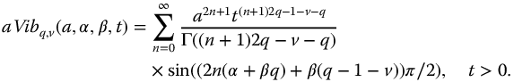
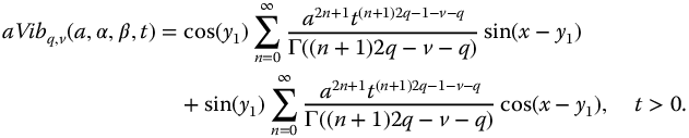
The meta-Vibration function,
, is defined as the imaginary part of the
-function; thus,
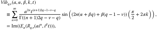
with t > 0, and  . Then, we have

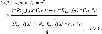
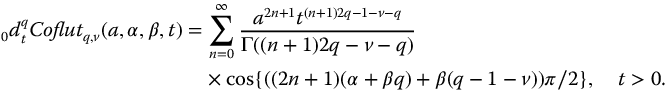
The generalized or meta-Rotation function similarly defines two new functions based on its real and imaginary parts; these are the meta-Flutter and meta-Coflutter functions, that is,
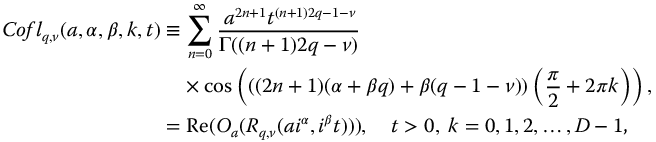
and
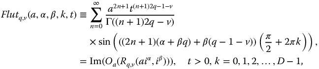
and where  is the product of the denominators
  .
.
In parallel with equation (9.31), we also have

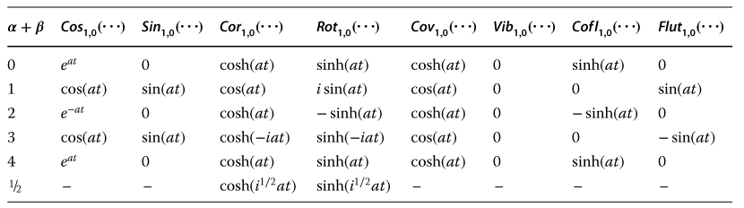
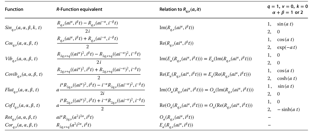
Table 9.1 presents special values for the fractional meta-trigonometric functions when  and
and  . The row
  can apply to the R1-hyperboletry, while the row
  can apply to the R1- and R2-trigonometries. The R3-trigonometry is a special case of the
  row. Of course, any of these rows may also be applied to noninteger values of
  and
and  . Continuing from Ref. [82] with permission of ASME:
Some observations may be made from the table. For example, for the
-function column all terms are of the form
. This may be shown as follows:
Similarly, for the
column, all terms are of the form
, since
Thus, we see that these functions are backward compatible with the hyperbolic functions with imaginary arguments. Other relationships are observed for the remaining columns.
Table 9.1 Special values of the generalized trignobolic functions
Source: Lorenzo 2009a [82]. Reproduced with permission of ASME.
For this table 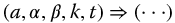 , also
  , – indicates only series description found.
9.3 Commutative Properties of the Complexity and Parity Operations
In this section, we demonstrate that the operations of determining the real/imaginary parts and even/odd parts of the parity functions may be interchanged. We start with the real part of  from equation (9.6); then, for
  , we have

where  . Expanding the summation yields

Collecting even and odd powers of a gives
However, we also observe that

and that

Now, from equations (9.29) and (9.42), we have

and from equations (9.32) and (9.43)

proving the assertion for these functions.
For the remaining functions, we begin with the imaginary part of  , from equation (9.7)

where 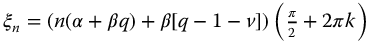 and
and  . Expanding this summation yields

Again, collecting even and odd powers of a gives

Here, we observe

and

Now, using equations (9.30) with (9.49)

and from equations (9.33) and (9.50),

completing the demonstration of the complexity–parity commutivity properties of 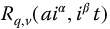 . These properties are summarized for the meta-trigonometric functions with t > 0 [83]:


where  and
and  refer to terms containing the odd and even powers of a, respectively.
9.3.1 Graphical Presentation – Parity Functions
Once again, it is not possible to show a representative display of the parity functions. The problem is exacerbated because the number of functions is doubled. Thus, the focus is on the effect of the generalizing variables  and
and  .
.
Figures 9.32–9.35 show the effect of the primary order variable, q, on the parity functions,  ,
,  ,
,  , and
, and  as a function of t time, with
  = 0.5 and
  = 0.5. Because
  = 1,
= 1,  = 0 corresponds to the R1-trigonometry and
  = 0,
= 0,  = 1 corresponds to the R2-trigonometry, the choice of
  = 0.5 and
  = 0.5 examines a new trigonometry sharing aspects of both R1- and R2-trigonometries. An observed feature of these figures is that increasing the order q increases the oscillatory behavior of the function in most cases. Note that the reversal of the first peak amplitude for
  for the
  - and
- and  -functions.
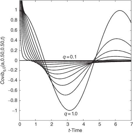
Figure 9.32 The effect of q for  , q = 0.1–1.0 in steps of 0.1, with a = 1, v = 0, k = 0,
  = 0.5,
  = 0.5.
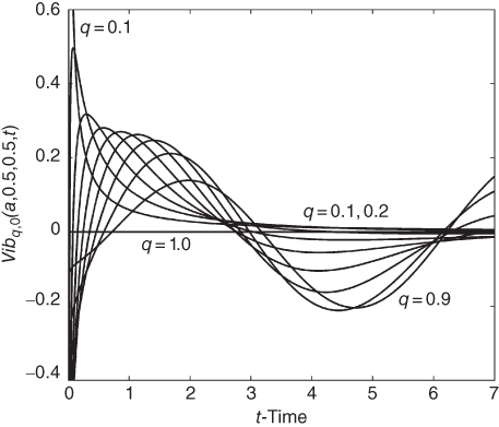
Figure 9.33 The effect of q for  , q = 0.1–1.0 in steps of 0.1, with a = 1, v = 0, k = 0,
  = 0.5,
  = 0.5.
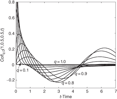
Figure 9.34 The effect of q for  , q = 0.1–1.0 in steps of 0.1, with a = 1, v = 0, k = 0,
  = 0.5,
  = 0.5.
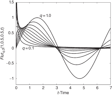
Figure 9.35 The effect of q for  , q = 0.1–1.0 in steps of 0.1, with a = 1, v = 0, k = 0,
  = 0.5,
  = 0.5.
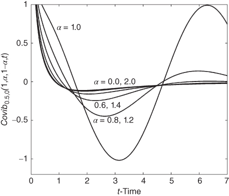
Figure 9.36 The effect of  and
and  ,
,  , for
, for  , with
  = 0.0–2.0 in steps of 0.2, and with q = 0.5, a = 1, v = 0, k = 0.
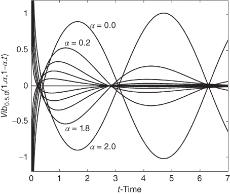
Figure 9.37 The effect of  and
and  ,
,  , for
, for  , with
  = 0.0–2.0 in steps of 0.2, and with q = 0.5, a = 1, v = 0, k = 0.
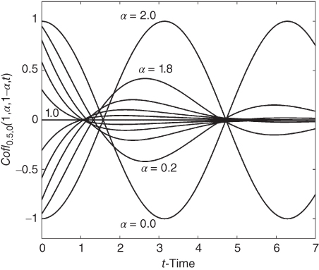
Figure 9.38 The effect of  and
and  ,
,  , for
, for  , with
  = 0.0–2.0 in steps of 0.2, and with q = 0.5, a = 1, v = 0, k = 0.
The effect of  and
and  , where
  , for
, for  ,
,  ,
,  , and
, and  functions is shown in Figures 9.36–9.39. For these figures,
  = 0.0–2.0 in steps of 0.2, and q = 0.5, a = 1, v = 0, k = 0. Note that the responses for the
  ,- and
  -functions are symmetric around
  , and the
  and
and  functions overlay themselves for
  , where
  .
.
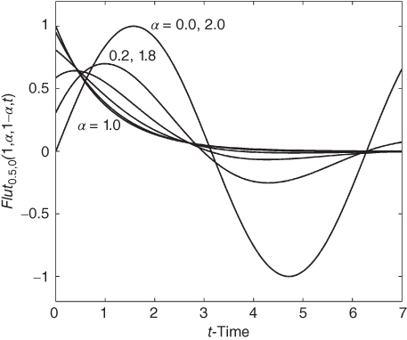
Figure 9.39 The effect of  and
and  ,
,  , for
, for  , with
  = 0.0–2.0 in steps of 0.2, and with q = 0.5, a = 1, v = 0, k = 0.
Figures 9.40 and 9.41 study the effect of a for  - and
- and  -functions with a = 0.25– 2.0 in steps of 0.25, and with q = 0.5,
  = 0.5,
  = 0.5, v = 0, k = 0.
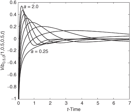
Figure 9.40 The effect of a for  , with a = 0.25–2.0 in steps of 0.25, and with q = 0.5,
  = 0.5,
  = 0.5, v = 0, k = 0.
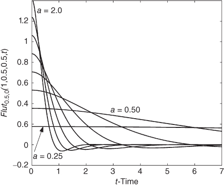
Figure 9.41 The effect of a for  , with a = 0.25–2.0 in steps of 0.25, and with q = 0.5,
  = 0.5,
  = 0.5, v = 0, k = 0.
Figures 9.42 and 9.43 study the effect of the differintegration variable, v, for the  - and
- and  -functions with v = −1.0 to 1.0 in steps of 0.25, and with q = 0.5, a = 1,
  = 0.5,
  = 0.5, k = 0.
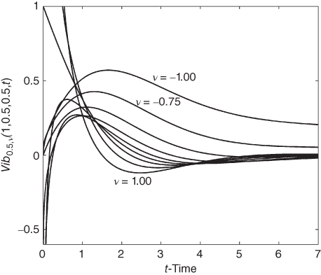
Figure 9.42 The effect of v for , with v = −1.0–1.0 in steps of 0.25, and with q = 0.5, a = 1, = 0.5, = 0.5, k = 0.

Figure 9.43 The effect of v for , with v = −1.0–1.0 in steps of 0.25, and with q = 0.5, a = 1,  = 0.5,
  = 0.5, k = 0.
Figure 9.44 considers the effect of the index variable k, for k = 0–4, with q = 3/5, a = 1,  = 0.5,
  = 0.5, v = 0. Note again the untypical symmetric responses resulting from the particular choice of q.
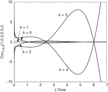
Figure 9.44 Effect of k, for k = 0–4, with q = 3/5, a = 1,  = 0.5,
  = 0.5, v = 0.
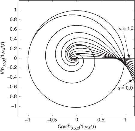
Figure 9.45 Phase plane showing the effect of  and
and  ,
,  , for
, for  versus
  with
with  = 0.0–1.0 in steps of 0.1, and with q = 0.5, a = 1, v = 0, k = 0, t = 0–9.
The remaining figures (Figures 9.45–9.52) are phase plane plots chosen to expose a few of the many varied possibilities. Figures 9.45 and 9.46 are phase planes showing the effect of  and
and  , where
  , for
, for  versus
  . For Figure 9.45,
  = 0.0–1.0 in steps of 0.1, and with q = 0.5, a = 1, v = 0, k = 0. For Figure 9.46,
  = 1.0 to 2.0 in steps of 0.1, also with q = 0.5, a = 1, v = 0, k = 0. All cases arrive from infinity and spiral into the origin except
  = 2.0, which is attracted to the unit circle. From Lorenzo [83]:
A particularly interesting, and important, pair of plots is found in Figures 9.47 and 9.48 for the
versus
phase plane. For both cases,
= 1.0–2.0 and q = 0.5, a = 1, v = 0, k = 0. While it is not obvious because of the change of scale between the pair, in Figure 9.47 as
is varied over the range
, with
, the responses start from the unit circle and diverge to infinity. In Figure 9.48 with
and all other variables the same, the responses start from the same identical points as in Figure 9.47 but are attracted to the origin. Furthermore, the slopes across the unit circle are preserved for each response. This behavior and its interpretation are discussed in more detail in Section 9.12.
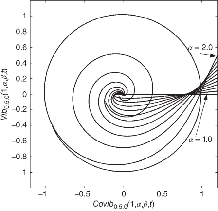
Figure 9.46 Phase plane showing the effect of and , , for versus with = 1.0–2.0 in steps of 0.1, and with q = 0.5, a = 1, v = 0, k = 0, t = 0–9.
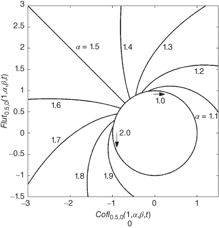
Figure 9.47 Phase plane showing the effect of  for
for 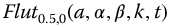 versus
  with
with  = 1.0–2.0 in steps of 0.1, and with q = 0.5, a = 1, v = 0,
  = 1, k = 0.
Source: Lorenzo 2009b [83]. Reproduced with permission of ASME.
Figure 9.48 . Phase plane showing the effect of  for
for  versus
 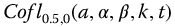 with
with  = 1.0–2.0 in steps of 0.1, and with q = 0.5, a = 1, v = 0,
  = 3, k = 0.
Source: Lorenzo 2009b [83]. Reproduced with permission of ASME.
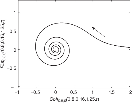
Figure 9.49 Phase plane for  versus
  with
with  = 0.16,
  = 1.25, and with q = 0.80, a = 0.8, v = 0, k = 0, t = 0–40.
Figure 9.50 Phase plane for  versus
  with
with  = 0.5, and with q = 1.09, a = 1.0, v = 0, k = 0, t = 0–19.
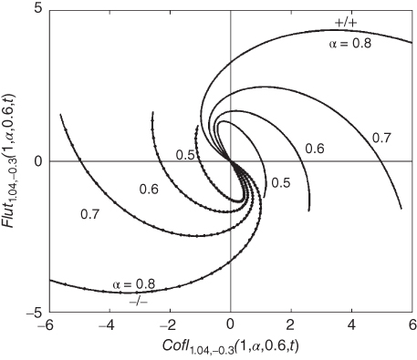
Figure 9.51 Phase plane for  versus
  and
and  versus
  with
with  = 0.5–0.8,
  = 0.6, and with q = 1.04, v = −0.3, a = 1.0, k = 0, t = 0–4.8.
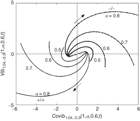
Figure 9.52 Phase plane for  versus
  and
and  versus
  with
with  = 0.5–0.8,
  = 0.6, and with q = 1.04, v = −0.3, a = 1.0, k = 0, t = 0–4.8.
Source: Lorenzo 2009b [83]. Reproduced with permission of ASME.
Figure 9.49 shows an interesting spiral converging to the origin that is similar to some of the classical spirals [64], pp. 188, 189. Figures 9.50–9.53 are phase plane plots of several barred spirals based on the parity functions. Figure 9.51 presents a phase plane for  versus
  and
and  versus
 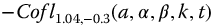 with
with  = 0.5–0.8. The spirals start at the origin and spiral out to infinity with increasing rate as
  increases.
Figure 9.53 Taxonomy of the fractional meta-trigonometric functions.
Source: Lorenzo 2009b [83]. Reproduced with permission of ASME.
Figure 9.52 is a very interesting phase plane plot for  versus
  and
and  versus
  with
with  = 0.5–0.8. The unusual feature here is that the departure is from the end of the spiral bar as
  increases. Such barred spiral behavior is of particular interest in the astrophysics of the galaxies. More such behaviors are studied in Chapter 18.
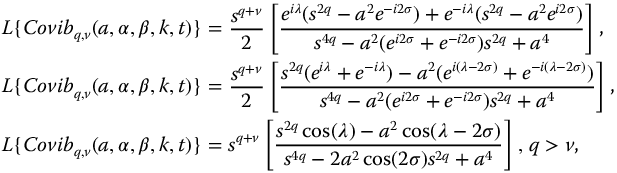
9.4 Laplace Transforms of the Fractional Meta-Trigonometric Functions
The development of the Laplace transform for the generalized functions parallels that of the previous trigonometries.
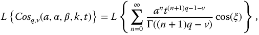
where  ,
,  , and where D is the product of the denominators
  , in equation (9.3), in minimal form. Because the series converges uniformly (see Sections 3.16 and 14.3), we may transform term-by-term. Thus,
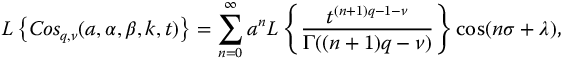
Continuing from Ref. [83]:
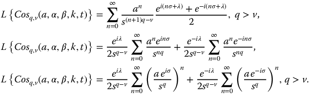
Recognizing the summations using equation (7.52) gives


where  ,
,  , and
, and  . The two forms, those of equations (9.65) and (9.66), are particularly useful.
The derivation for the Laplace transform of  proceeds in a similar manner:

with  ,
,  and giving the results
and

where  and
and  .
.
The Laplace transform for the  follows.
Continuing from Ref. [83]:

where  , and
, and  is the product of the denominators
 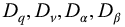 , in minimal form and where
 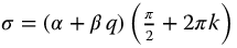 and
and 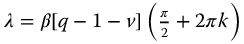 .
.
Similarly, for the  , we have


where  , and
, and  .
.
The Laplace transform for the  follows:


where  , and
, and  .
.
The derivation for the  is similar to that for
  and yields


where  , and
, and  .
.
This collection of Laplace transforms generalizes those derived for the previous trigonometries. Comparison of these transforms with the parallel results for the R3-trigonometric functions shows that the transforms are structurally the same and the R3 results may be had by the substitutions  . Table 9.2 summarizes the Laplace transforms of the meta-trigonometric functions.
Table 9.2 Summary of the meta-trigonometric functions
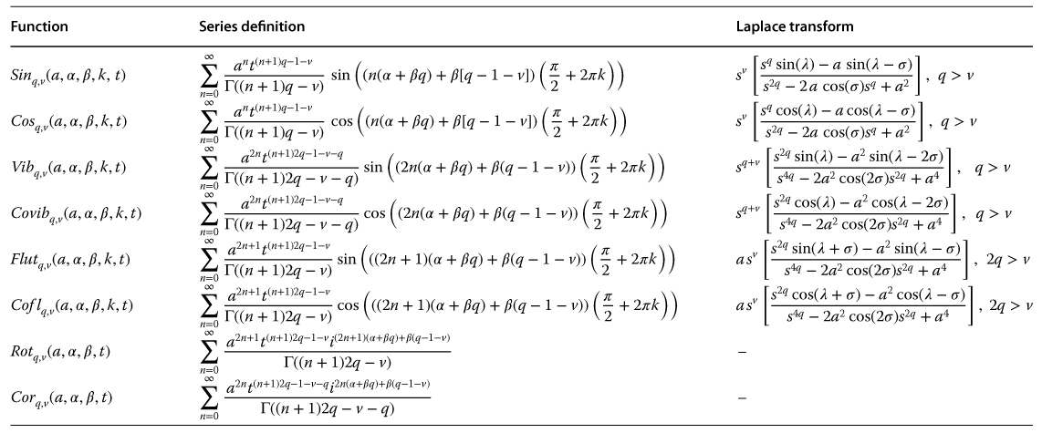
Source: Lorenzo 2009b [83]. Reproduced with permission of ASME.
 ,
,  ,
,  ; D is the product of the denominators of
  with repeated multipliers removed.
9.5 R-Function Representation of the Fractional Meta-Trigonometric Functions
The fractional exponential or R-function representation of the trigonometric functions is useful for analysis and numerical computation. Continuing from Ref. [83]:
Now, from the definition of
, we have for t > 0
Now,
Applying equation (3.124), namely 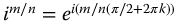 , yields
Then,
The summations are recognized as R-functions giving the result

Applying equation (3.121) simplifies the result to
The remaining functions are determined in a similar manner and are listed in two forms, t real and complex; thus, we have

or


or


or

or
or

Finally, summarizing the results of equations (9.22) and (9.24)
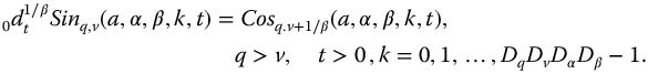
9.6 Fractional Calculus Operations on the Fractional Meta-Trigonometric Functions
For the fractional differintegrations that follow, it is assumed that the integrated function, and all of its derivatives, are identically zero for all t < 0. Continuing from Ref. [83]:
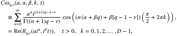
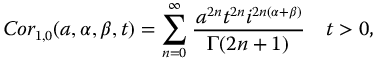
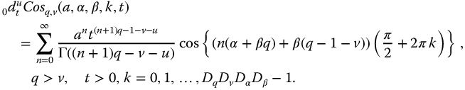
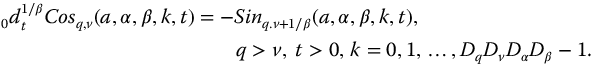
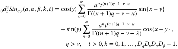
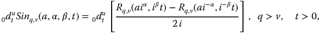
9.6.1 Cosq,v(a, α, β, k, t)
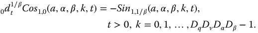
The u-order differintegral of  is determined for t > 0 as
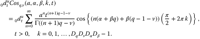
We may differintegrate term-by-term (see Section 3.16); thus,

Applying equation (5.37), that is,
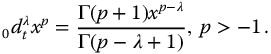
Thus equation (9.96) becomes
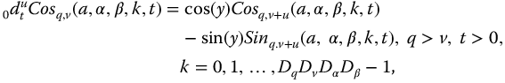
From the sum and difference formulas for the integer-order trigonometry, the following identities may be derived:

and

Now, in equation (9.98), let  , and
, and  , with
  ; then applying equation (9.99) gives

The summations are recognized as  and
and  , respectively, yielding the final result
where  . Taking
 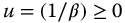 , we have
  and
and  giving
Now, taking 
An alternative development of the result of equation (9.103) is obtained as follows:
by the differentiation equation (3.114)

When  , we have
which is recognized as

which is identically equation (9.104) when  .
.
9.6.2 Sinq,v(a, α, β, k, t)
Determination of the differintegral for the  -function proceeds in a manner similar to that of the
  . Then, the u-order differintegral of
  is determined as


Application of equation (9.97) to this equation gives
In equation (9.110), let 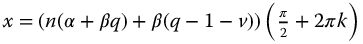 and
and  ,
,  ; then applying equation (9.100), we have
The summations are seen to be  and
and  , respectively, yielding the final result

where  . Taking
  , we have
  and
and  , giving
Furthermore, taking 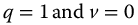 gives
gives
The R-function-based development of the result of equation (9.113) is obtained based on equation (9.84) as
by the differentiation equation (3.114)

When  and k = 0, this yields the same result as equation (9.113).
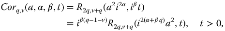
9.6.3 Corq,v(a, α, β, t)
The u-order differintegral for the  -function is determined, using definition (9.2.8), as


Application of equation (9.97) to this equation gives


with  , and where the summation has been recognized as an
  -function, to yield the final result. In terms of the R-function, we have

or

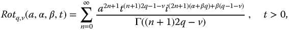
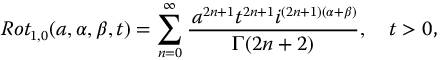
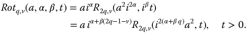
9.6.4 Rotq,v(a, α, β, t)
Determination of the differintegral for the  -function proceeds in a manner similar to that of
  . Then, the u-order differintegral of
  is determined as


Application of equation (9.97) to this equation gives

The summation is seen to be  , yielding

In terms of the R-function representation, we have
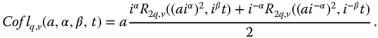
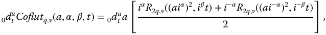
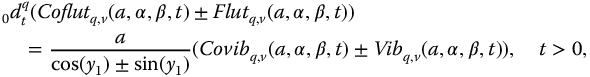
9.6.5 Coflutq,v(a, α, β, k, t)
In this section, we determine the differintegral of the Coflutter function. The u-order differintegral of  is determined as


Application of equation (9.97) to this equation gives

with  . Now, in equation (9.128), let
  ,
,  , also, let
  ; then, applying equation (9.99), we have
The summations are recognized as  and
and  , yielding the desired differintegral form

where  . For the special case with
  , we have
  and
and  , giving

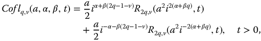
Taking  in equation (9.130) gives the general form for the differintegral of the Coflutter function as

Furthermore, with  , we have
The alternative R-function-based development of the results of equation (9.90) is obtained as
by the differentiation equation (3.114)

For the case  ,
,


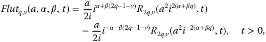
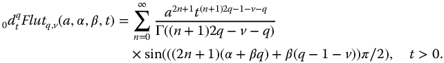
9.6.6 Flutq,v(a, α, β, k, t)
The  -order differintegral of
  is determined as

where 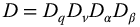 is in minimal form.
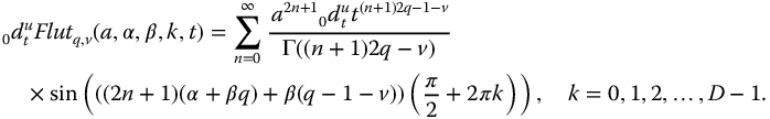
Applying equation (9.97) to this equation gives
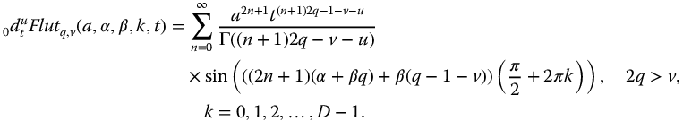
Now, in equation (9.139), let  ,
,  and let
  ; then, applying equation (9.100), we have
with  . The summations are recognized as
  and
and  , respectively, yielding the final result
where  . For the special case where
  , we have
  and
and  , giving

The alternative R-function-based development of the results of equation (9.92) is obtained as follows:

Application of the differentiation equation (3.114) gives the result
With  , we have

or

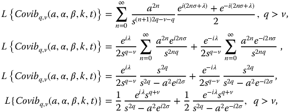
9.6.7 Covibq,v(a, α, β, k, t)
The  -order differintegral of the
  is determined as follows:


Application of equation (9.97) to this equation gives

Now let  ,
,  in equation (9.147) and let
  ,
,  ; then, applying equation (9.99), we have

The summations are seen to be  and
and  , respectively, yielding the key result

where  . When
  we have
  and
and  ; thus,

The R-function-based differintegral is obtained as

By the differentiation equation (3.114)

When  , we have

The right-hand side is seen to be  , thus validating equation (9.150).
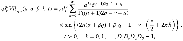
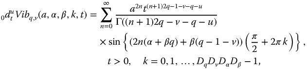
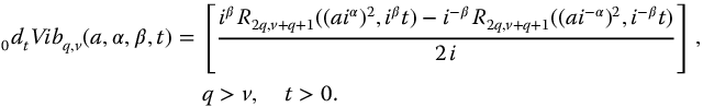
9.6.8 Vibq,v(a, α, β, k, t)
The  -order differintegral of the generalized vibration function,
  , is derived as follows:

Application of equation (9.97) to this equation gives
with  . Now, let
  ,
,  ,
,  , in equation (9.154). Then, applying equation (9.100), we have

The summations are recognized as  and
and  , respectively, yielding the key result

where  . When
  , we have
  and
and  , giving

Now, taking  in equation (9.156),

With both  and with
  , we have

However, if additionally  ,
,  ; therefore, we have

where  . The alternative R-function-based development of the results of equation (9.88) is obtained as

by the differintegration equation (3.114)

When  , we have
Tables 9.2 and 9.3 summarize the various properties of the meta-trigonometric functions.
Table 9.3 Summary of the meta-trigonometric functions
Source: Lorenzo 2009b [83]. Reproduced with permission of ASME.
 ,
,  ; D is the product of the denominators of
  in minimum form.
9.6.9 Summary of Fractional Calculus Operations on the Meta-Trigonometric Functions
For ease of reference the fractional calculus operations are summarized here. The derivations are for t > 0, and  and
and  :
:


9.7 Special Topics in Fractional Differintegration
In this, and previous chapters, fractional differintegrals of the fractional trigonometric functions have been derived. In all cases, the fractional differintegration has started from t = 0. Because the functions are zero for t < 0, initialization or history effects have not been an issue. However, when a function does not start from zero or is segmented, such as
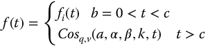
and preceded by another different function, fractional differintegrations must consider the initialization effects caused by the preceding function. Clearly, there will be times when it is desired to start a fractional differintegration at times other than t = 0. The reader is cautioned that fractional differintegration differs from integer-order integration in this important regard. Detailed analysis of these important differences is addressed in Appendix D.
9.8 Meta-Trigonometric Function Relationships
This section determines generalized identities for the fractional meta-trigonometric functions in terms of the fractional exponential functions. These are parallel to the very basic identities presented in equations (1.18) and (1.19). The results will, of course, apply to all particular fractional trigonometries that may be derived by specializing the results of this chapter.
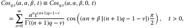
9.8.1 Cosq,v(a, α, β, t) and Sinq,v(a, α, β, t) Relationships
The generalized fractional Euler equation, with k = 0, for the  - and
- and  -functions was determined in Section 9.1 as

The complementary generalized fractional Euler equation, with k = 0, can be determined by expanding  , in a manner similar to the expansion from equation (9.1) to (9.5), or by subtracting equation (9.84) from (9.82), which gives

Continuing from Ref. [83]:

Adding and subtracting the resultant equations provides the following two identities:


From the result of equation (9.176), it is clear that because  and
and  are real, the product
  must also be real. Thus, we note that
  is the complex conjugate of
  . These identities (9.176) and (9.177) are broad generalizations of
  and
and  from the ordinary trigonometry. This may be shown by taking
  in equations (9.176) and (9.177).
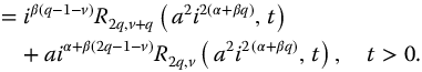
9.8.2 Corq,v(a, α, β, t) and Rotq,v(a, α, β, t) Relationships
Consider, from equation (9.124) with 

The summation is recognized as  yielding

From equation (9.125), we have

Therefore,

Continuing from Ref. [83]:
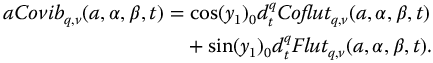
9.8.3 Covibq,v(a, α, β, t) and Vibq,v(a, α, β, t) Relationships
Equations (9.86) and (9.88) are rewritten in the following form:


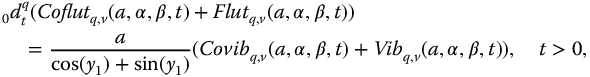
Adding these equations gives the generalized fractional semi-Euler equation for the Vibration functions as

or

While subtracting yields the generalized complementary semi-Euler equation

or

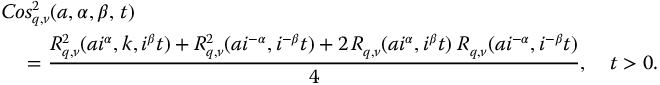
The terminology semi-Euler is used because of the q to q/2 relationship between the right- and left-hand sides of the equations. Squaring equations (9.86) and (9.88) yields

Adding and subtracting these equations give


meta-identities relating the  and
and  -functions.
9.8.4 Coflq,v(a, α, β, t) and Flutq,v(a, α, β, t) Relationships
The  - and
- and  -functions can also be related. We rewrite equations (9.90) and (9.92) as follows:

and

Adding equations (9.192) and (9.193) gives

Alternatively,

the generalized fractional semi-Euler equation for the Flutter functions. Subtracting equation (9.193) from (9.192) yields

or

the generalized complementary fractional semi-Euler equation for the Flutter functions. The functions as represented in equations (9.90) and (9.92) are squared to give

The sum and difference of these equations yield


generalized identities relating the  and
and  -functions.
9.8.5 Coflq,v(a, α, β, t) and Vibq,v(a, α, β, t) Relationships
Taking  and k = 0 in equation (9.139) gives
Now,
Let  and
and  with
with

Then, we may write equation (9.203) as
More succinctly,

Taking  , and k = 0 in equation (9.204) gives
Now,

Using the same substitutions  and
and  with
with  into equation (9.208) gives
Adding equations (9.206) and (9.209) yields the interesting result
where  . Subtracting equation (9.206) from (9.209) gives the complementary result, which may be combined into the single identity
where again  .
.
9.8.6 Cosq,v(a, α, β, t) and Sinq,v(a, α, β, t) Relationships to Other Functions
The following relationships are presented without proof. They may be easily shown by substitution into the defining series and with the use of equations (9.99) and (9.100):


For the principal functions, we have

where  .
.

where  .
.
These are but a few of the many relationships possible for the meta-trigonometric functions. Many other relations paralleling the multiple- and fractional-angle formulas from the integer-order trigonometry and more are yet to be derived.
9.8.7 Meta-Identities Based on the Integer-order Trigonometric Identities
Because the series definitions of the meta-trigonometric functions contain the periodic cosine and sine functions, inter-relationships may be determined for these functions. This section determines meta-identities based on these relationships for the  - and
- and  -functions. Identities such as
  and
and  are possible bases, as are the following identities provided by Spanier and Oldham [116], pp. 298–299 from the integer-order trigonometry:

Identities for the  -functions are considered first.
9.8.7.1 The cos(−x) = cos(x)-Based Identity for Cosq,v(a, α, β, t)
The question to be answered is: For given values of q and v what values for  and
and  will provide an identical function with parameters
  and
and  ? In other words, under what conditions will

From the definition of  ,
,

This will occur when for all n

Now, from the classical trigonometry using  , this requires

This equality must also hold for n = 0; thus,

This result substituted into equation (9.221) yields

from which

Thus, the final result is

9.8.7.2 The sin(−x) = − sin(x)-Based Identity for Sinq,v(a, α, β, t)
Here, we wish to find conditions under which

From the definition of  ,
,

Considering the sine arguments

This equality must also hold for n = 0; thus,

This result is now substituted into equation (9.226) giving

Combing the argument result with the sign change for  yields the final result

9.8.7.3 The Cosq,v(a, α, β, t) ⇔ Sinq,v(a, α, β, t) Identity
Selected arguments of the classical cosine and sine functions in the  - and
- and  -functions also lead to identities. For this study, we consider

and

Then  when
when

From the classical trigonometry (equation (9.217), we have 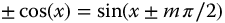 , where
 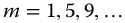 . Applying the identity to equation (9.230) gives

Comparing arguments
Again, the relationship must hold for n = 0; thus,
This result substituted into equation (9.232) yields
Thus, the resulting meta-trigonometric identity is given by

9.8.7.4 The sin(x) = sin(x ± mπ/2)-Based Identity for Sinq,v(a, α, β, t)
For  , identities will occur when

Based on the definition of  ,
,

We require

Here, from equation (9.217), we use the identity  , where
  ; thus,

Comparing arguments

Since the relationship must also hold when n = 0,
Substituting equation (9.240) into (9.239) gives
Thus, we have the identity

Clearly other, possibly stronger, identities of this type are possible. Importantly, because the series defining the parity functions also contain integer-order sine and cosine terms, similar identities may be created for them. Continuing from Ref. [83]:
9.9 Fractional Poles: Structure of the Laplace Transforms
Consider the Laplace transform of the Covibration function. From equations (9.72) and (9.71), we have
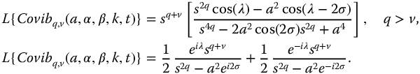
This can be further resolved to
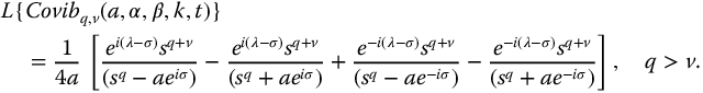
From the transform pair (equation (244), it may be seen that the  may be composed by a weighted sum of four R-functions or four complex fractional poles. The transforms of all of the fractional meta-trigonometric functions may be similarly decomposed.
9.10 Comments and Issues Relative to the Meta-Trigonometric Functions
The previous sections of this chapter have presented the definitions, Laplace transforms, special properties, and identities for the meta-trigonometry based on the fractional exponential function,  . From these meta-definitions and properties, the analyst may specialize the variables q, v,
  , and
, and  to obtain particular fractional trigonometries or hyperboletries. The same variables substituted into the meta-transforms, meta-identities, and so on will yield those transforms and identities specialized to the particular fractional trigonometry.
The mathematical process that was used to generate the meta-functions is shown graphically in Figure 9.53. The a and t variables of fractional exponential function,  -function expressed in series form, are generalized to the complex forms shown in the level 2 box. Two paths are shown from level 2 to level 3. The left path takes the real and imaginary parts of the series while the right path takes the even and odd powered terms of the series. From level 3 to 4, following the left path, four new functions are generated by taking the even and odd powered terms of the cosine and sine series. Following the right path, the same four functions may be generated by taking the real and imaginary parts of the complex corotation and rotation functions.
Thus, the process described produces eight functions, six of which are real, and the complex corotation and rotation functions. It is noted that at level three, the leading term of the Laplace transform denominators is 2q while at level four it doubles to 4q. It is noted that the mathematical process observed here is fractal and may be repeated indefinitely to finer and finer resolution of  .
.
9.11 Backward Compatibility to Earlier Fractional Trigonometries
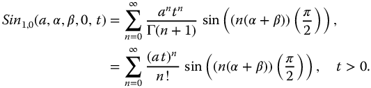
The generalized fractional or meta-trigonometry as defined here contains both the R2 and R3-fractional trigonometries discussed previously. For example, to obtain the R2-functions, we need only set  and
and  in the meta-functions; that is, the basis for the trigonometry is
  . Similarly, for the R3-trigonobolic functions, we set
  , giving the basis
  .
.
The generalized R1-trigonometry is not, however, directly compatible with definitions forwarded for the R1-trigonometry, which was conceived prior to the generalized theory. However, the principal R1-trigonometric functions are compatible with the meta-trigonometry. It is noted that both versions have the basis  .
.
The choice q = 1, v = 0,  , and
, and  will yield the functions and identities associated with the classical trigonometry (albeit with new names).
The Covibration function is the real and even part with respect to the powers of a of  and, therefore, is a proper successor to the cosine function of the classical trigonometry and the Flut function is imaginary and odd part with respect to the powers of a and, therefore, is an appropriate successor for the sine function. Thus, the
  -function in the meta-trigonometry is only the real part of the
  -function and
  is only the imaginary part of the
  -function; that is, the parity operations have not been applied. The taxonomy chart of Figure 9.53 illustrates the relationships.
9.12 Discussion
The meta-trigonometry expands the fractional trigonometries and fractional hyperboletry from the four bases of Chapters 5–8 to the complete infinite set. The defined functions are useable for the study of many dynamic processes and for the solution of many classes of fractional differential equations via the Laplace transforms of the meta-functions. Considerable study will be required to determine which of the bases are important and where they may be applied. While the fractional trignoboletries release us from the constraints associated with the unit circle, many challenges must be met for the area to develop to mathematical maturity, some follow.
The foregoing material has only dealt with the primary functions:  ,
,  , and so on. The ratio and reciprocal functions (i.e., tan, cotan, etc.) associated with the six primary functions still need to be defined and to have their properties developed. The task is daunting as there are 36 such functions. The next chapter provides some thoughts on this topic.
Development of inverse function definitions (in series form) is problematic since in most cases no repetitive principal cycle exists, and the inverse functions are one-to-many mappings. Software methods, however, may allow us to temporarily bypass this step for practical application. A more detailed discussion of this topic is found in Chapter 20.
The existence of orthogonal function sets outside of the classical trigonometry will need to be explored. Furthermore, will the classical definitions of orthogonality be adequate or will new fractional-based definitions be needed?