Chapter 8
The R3-Trigonometric Functions
In the integer-order trigonometry, replacing the frequency parameter a by the imaginary parameter  toggles the functions back and forth between the trigonometric and the hyperbolic functions. For example,

and for the cosine function

Parallels to this were found for the  -trigonometry with the
  -hyperboletry. However, this is not the case relative to the
  -trigonometry. This chapter develops the effect of an imaginary frequency parameter and an imaginary time parameter in the R-function.
8.1 The R3-Trigonometric Functions: Based on Complexity
The basis for definition of the R1-trignometric functions is to allow  . The R2-trigonometric functions are based on
  . The obvious question is: What is the nature of the results when both
  and
and  ? This assumption is the basis of the R3-trignometric functions. We start by separating
  into real and imaginary parts. Thus, we consider


Now, for rational q and v, we may write

Thus,

where  ,
,  , and
, and  . Therefore, equation (8.2) may be written as

where k is included in the R-function argument to reflect its presence in  on the right-hand side. Then, by similarity to equations (7.6) and (7.7), we define


Thus, these definitions are quite similar to those for  and
and  , differing from their R2 counterparts only by the presence of an extra “n” in the arguments of the circular functions. As with the R2-trigonometric functions, we define the principal functions for t > 0, as


Combining equations (8.4)–(8.6) gives

Figure 8.1 shows the principal  - and the
  -functions for values of q between q = 0.2 and q = 1.0, with a = 1.0 and v = 0. We observe from Figure 8.1 that for q = 1 and
  we have
  , and we can see that
  . These results are readily verified by appropriate substitution into equations (8.7) and (8.8). The character of these functions changes considerably for
  , which is illustrated in Figure 8.2. For
  and greater, the principal
  - and
- and  -functions also grow in oscillation amplitude.

Figure 8.1  and
and  versus t-Time for a = 1, k = 0, v = 0, q = 0.2–1.0 in steps of 0.2.

Figure 8.2  and
and  versus t-Time for a = 1, k = 0, v = 0, q = 1.0–1.5 in steps of 0.1.
In Figures 8.3 and 8.4, we study the effect of changes in the a parameter on the principal  - and the
  -functions for values of q = 0.25 and 0.75, respectively. As seen in the R1 and R2 trigonometries, the effect of increasing a leads to faster transient responses of the trigonometric variables. The effect of the differintegration order variable, v, is presented in Figures 8.5 and 8.6 for values of q = 0.25 and 0.75, respectively. Here, we see that v not only changes the transient rate of response of the trigonometric functions, but also the nature of the response, in particular when the sign of v changes.

Figure 8.3 Effect of a,  , and
, and  versus t-Time for a = 0.25–1.0 in steps of 0.25, with q = 0.25, k = 0, v = 0.

Figure 8.4 Effect of a,  , and
, and  versus t-Time for a = 0.25–1.0 in steps of 0.25, with q = 0.75, k = 0, v = 0.
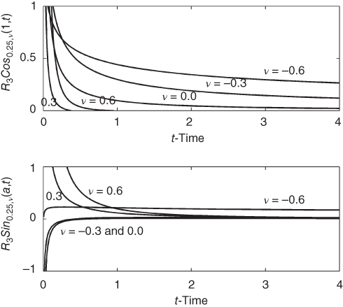
Figure 8.5 Effect of v,  , and
, and  versus t-Time for v = −0.6–0.6 in steps of 0.3, with q = 0.25, k = 0, a = 1.

Figure 8.6 Effect of v,  , and
, and  versus t-Time for v = −0.6–0.6 in steps of 0.3, with q = 0.75, k = 0, a = 1.
The effect of k, for  , with k = 0 to 6 in steps of 1, and q = 5/7, a = 1.0, v = 0 is shown in Figure 8.7. In this case, strong symmetry is again seen. It has been observed that the
  -function maintains this symmetry for
  with n an odd integer.

Figure 8.7 Effect of k, for  , with k = 0–6 in steps of 1, q = 5/7, a = 1.0, v = 0.
Figure 8.8 shows a phase plane for  versus
  for q = 1.0 to 2.0. In this figure, all cases start from the origin. The cases with
  return to the origin, while those for
  diverge with increasing rates.

Figure 8.8 Phase plane  versus
  for q = 1.0–2.0 in steps of 0.2, with a = 1.0, v = 0, and t = 0–7.0.
8.2 The R3-Trigonometric Functions: Based on Parity
We now consider  based on parity of the exponent of a. Then, equation (8.1) is written as

The summation becomes

Forming two summations by separating terms with even and odd powers of  , we may write


We note in passing the identity

which after application of equation (3.119) becomes

For  , equation (8.13) is rewritten as

where the summations are separated into even and odd powers of  in (8.12). In parallel with the development of the
  -trigonometric functions, and based on equations (8.13) and (8.14), we define the
  -Corotation and
  -Rotation functions as the summations with even and odd powered a terms, respectively:


We now use the real and imaginary parts of these functions to define the four new real fractional trigonometric functions that parallel those defined for the  -trigonometry.
The  -function is rewritten as

Applying equation (3.123) to  with q and v rational, we have

where  and
and  are assumed to be rational and irreducible and M/D is in minimal form. Thus,

where  . Then
  may be written as

The real part of the  is defined as the
  -Covibration function

The imaginary part of equation (8.19) defines the  -Vibration function

We now examine the nature of these functions when  and
and  :
:

and

The  -function (equation (8.17) is now written as

Applying equation (3.123) to  with q and v rational, we have

where  and
and  are assumed to be rational and irreducible and M/D is in minimal form. Thus

where  . Then,
  may be written as

Thus, we define the real part as the  -Coflutter function

and the imaginary part as the  -Flutter function

Again, we examine the nature of these functions when  , and
, and  , then

and

The backward compatibility, that is, the  , and
, and  evaluation, of the
  -functions for t > 0, is summarized as


Thus, we see that these functions are backward compatible with the common exponential and the hyperbolic functions and indeed might be considered as the  -hyperbolic functions.
Here, the complexity and parity properties of  in terms of the
  -trigonometric functions are summarized; for t > 0


where  and
and  refer to the forms with terms containing the even and odd powers of a. Also we see that, by design, these forms exactly parallel those of the related
  -functions. Similar to the
  case, the commutative property of equations (8.39)–(8.42) are readily proved by taking the real and imaginary parts of equations (8.16) and (8.17) and relating them to the even and odd parts of equations (8.7) and (8.8).

Figure 8.10  versus t-Time for a = 1, v = 0, k = 0, and q = 0.1–0.5 in steps of 0.1.

Figure 8.11  versus t-Time for a = 1, v = 0, k = 0, and q = 0.1–0.5 in steps of 0.1.
The  -,
-,  -,
-,  -, and
  -functions are presented in Figures 8.9–8.12 for
  , with a = 1, and v = 0. In the figures, and validated by substitution in the appropriate series, we observe
  and
and  . Figure 8.13 presents a phase plane
  versus
  for q = 0.5–1.5. For q > 0.5, the functions spiral out from the origin with increasing rate as q increases.

Figure 8.9  versus t-Time for a = 1, v = 0, k = 0, and q = 0.1–0.5 in steps of 0.1.

Figure 8.12  versus t-Time for a = 1, v = 0, k = 0, and q = 0.1–0.5 in steps of 0.1.
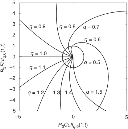
Figure 8.13 Phase plane  versus
  for q = 0.5–1.5 in steps of 0.1, a = 1.0, k = 0, v = 0, t = 0–10.
The phase plane  versus
  for q = 0.5–1.5 is presented in Figure 8.14. For
  the curves approach from infinity and are repelled before reaching the unit circle at q = 0.5 outward back toward infinity. For q > 1, the curves leave the origin and spiral out to infinity with increasing rate. The q = 1 case starts at the unit circle and proceeds to infinity. Also, it may be shown that
  .
.

Figure 8.14 Phase plane  versus
  for q = 0.5–1.5 in steps of 0.1, a = 1.0, k = 0, v = 0, t = 0–12.
8.3 Laplace Transforms of the R3-Trigonometric Functions
The development of the Laplace transform for the R3-trigonometric functions parallels that of the  -functions. Thus, we state the results in normal and factored form without development.


where  and
and  , with
  . Comparison of these transforms with the parallel results for the R2-trigonometric functions shows that the transforms are structurally the same and vary from each other primarily in the coefficient of the
  term in the denominator. We will later see that this influences the damping behavior of the transform.
Note that most of the figures presented in this and previous chapters are of results in the stable domain that is of trigonometric order,  for the complexity functions. The reader is encouraged to numerically explore values of q > 1 as many important applications are found there; see, for example, Chapters 17–20. For the parity functions, explore q > 1/2.
8.4 R3-Trigonometric Function Relationships
This section determines expressions for the  -trigonometric functions in terms of the fractional exponential functions. These expressions parallel the basic equations (1.18) and (1.19). Some special R-function relationships also result. The organization of the subsections of this section has been set by the ease of development of relationships.
8.4.1 R3Cosq,v(a, t) and R3Sinq,v(a, t) Relationships and Fractional Euler Equation
This section develops some important properties of the R3-trigonometric functions. We observe from equations (8.4)–(8.6) that

This equation parallels the form of equations (6.15) and (7.12) for the  and R2-trigonometries, respectively. Consider now the
  -function as defined in equation (8.5), that is,

Applying definition (1.18), we may write

Now, by equation (3.124),  , and (3.127), we have

This may be written as


Recognizing the summations as  -functions, we have

or applying equation (3.119)

This equation generalizes equation (1.18) in the ordinary trigonometry. It could also serve as a definition of  .
.
The development for the  -function follows in similar manner, yielding

This equation exactly parallels equation (1.19) in the ordinary trigonometry. It could also serve as a definition of  . Solving for
  using both equations (8.58) and (8.59) yields equation (8.51) and subtracting (8.59) from (8.58) gives, for t > 0

the companion to equation (8.51). Now, squaring equations (8.58) and (8.59) yields


Adding and subtracting equations (8.61) and (8.62) gives

and

These equations parallel equations (6.23) and (6.24) and provide additional generalizations of the equations  and
and  .
.
8.4.2 R3Rotq,v(a, t) and R3Corq,v(a, t) Relationships
As previously mentioned,  and
and  are complex functions. From the definitions (equations (8.15)–(8.17), we have for t > 0

We observe that the summations of equations (8.16) and (8.17) are R-functions of complex arguments, and using equation (3.118), we may write


Combining the results of equations (8.66) and (8.67) with equation (8.65) gives the following identity:

8.4.3 R3Coflq,v(a, t) and R3Flutq,v(a, t) Relationships
The analysis starts by replacing the cos function in the definition of  in equation (8.26). Then, using logic similar to the process used for the
  , that is, equations (8.53) to (8.57), we have for t > 0

where  ,
,  with t > 0, and
  . Applying equation (3.124) to the exponential functions, we have
  and
and  . Thus, we have

Applying equation (3.119) to these R-functions, we write the final result as

The  -function is derived in a similar manner. We give the final result

We now derive some additional properties of these functions. Rewrite equations (8.70) and (8.71) as


Adding equations (8.72) and (8.73) gives

This equation may be considered as a fractional “semi-Euler” equation. Subtracting equation (8.72) from equation (8.73) and using (8.17) yields the complimentary equation

Now, in equations (8.74) and (8.75), let  ; then,

and

which may be considered as fractional “semi-Euler” equations. Replacing  in equation (8.9) gives

Comparing the real and imaginary parts of this equation with equation (8.76), we observe that

and

8.4.4 R3Covibq,v(a, t) and R3Vibq,v(a, t) Relationships
This analysis starts by rewriting equation (8.20), the  -function, as

where  and
and  . This becomes

Since  and
and  , we have

Applying equation (3.119) to both terms gives

The derivation for the  follows in a similar manner; thus,

Additional properties of these functions are now determined. Rewrite equations (8.81) and (8.82) as


Adding equations (8.83) and (8.84) gives

This equation may also be considered as a fractional “semi-Euler” equation. Subtracting equation (8.84) from equation (8.83) yields the complimentary equation

Now, in equation (8.85), let  ; then,

Alternatively, we may write

Replacing a in equation (8.51) by  gives
gives

Comparing this result with equation (8.88), we observe that

and

Rewrite equation (8.85) as

Relating the real and imaginary parts of equations (8.92) and (8.75), we obtain


exposing relationships between the parity functions. It should be remembered, because of the role of the v as an order variable, that these relationships also represent fractional differintegration relationships.
These are but a few of the many relationships possible for the  -trigonometric functions. Many other relations paralleling the multiple-angle and fractional-angle formulas from the integer-order trigonometry and more are yet to be derived.
8.5 Fractional Calculus Operations on the R3-Trigonometric Functions
8.5.1 R3Cosq,v(a, k, t)
The  -order differintegral of
  is determined for t > 0 as

Based on Section 3.16, we may differintegrate term-by-term:

Applying equation (5.37), that is,

valid for all  . Differintegrating equation (8.96) term-by-term yields

From the sum and difference formulas for the integer-order trigonometry, the following identities are derived:

and

Now, in equation (8.98), let  ,
,  , also, let
  , then applying equation (8.99)

The summations are recognized as  and
and  , respectively, yielding the final result

where  . Taking
  we have
  and
and  giving

Now, taking  gives
gives

which evaluates to

An alternative development of the result of equation (8.103) is obtained as follows:

by the differintegration equation (3.114)

When  , we have

which is recognized as

8.5.2 R3Sinq,v(a, k, t)
Determination of the differintegral for the  -function proceeds in a similar manner to the
  . Then, the
  -order differintegral of
  is determined as


Application of equation (8.97) to this equation gives

Now, in equation (8.112), let  ,
,  , also, let
  ; then applying equation (8.100), we have

The summations are recognized as  and
and  , respectively, yielding the final result

where  . Taking
  , we have
  and
and  , giving

Taking  yields

which evaluates to

again the expected result.
The alternative R-function-based development of the result of equation (8.114) is obtained based on equation (8.59), as

by the differintegration equation (3.114)

When  , we have

which is recognized as

8.5.3 R3Corq,v(a, t)
Determination of the derivative for the  -function proceeds in similar manner to
  . Then, the
  -order differintegral of
  is determined, using definition (8.16), as


Application of equation (8.97) to this equation gives

The summation is recognized as both an R-function and as an R3Rot-function, yielding the final result

8.5.4 R3Rotq,v(a, t)
Determination of the derivative for the  -function proceeds in a manner that is similar to
  . Then, the
  -order differintegral of
  is determined as


Application of equation (8.97) to this equation gives

The summation is recognized as both an R-function and as an R3Rot-function, yielding

8.5.5 R3Coflutq,v(a, k, t)
In this section, we determine the derivative of the  -function. The
  -order differintegral of
  is determined as

Differintegrating term-by-term,

Application of equation (8.97) to this equation gives

Now, in equation (8.126), let  ,
,  , also, let
  ; then applying equation (8.99), we have

The summations are recognized as  and
and  yielding the desired derivative form

where  . Taking
  , we have
  and
and  , giving

Taking  , in equation (8.127), gives the derivative as

and with  we have

However,  , thus

The alternative R-function-based development uses equation (8.70) to obtain

by the differintegration equation (3.114)

When  , we have for t > 0

as seen in equation (8.128).
8.5.6 R3Flutq,v(a, k, t)
The  -order differintegral of
  is determined as

Application of equation (8.97) to this equation gives

Now, let  , also let
  ; then, applying equation (8.100), we have

The summations are recognized as  and
and  , respectively, yielding the final result

where  . Taking
  , we have
  and
and  , giving

Taking  , in equation (8.135), we obtain

When we also have  , this becomes

However,  , thus indicating that

The alternative R-function-based development uses equation (8.71) to obtain

by the differintegration equation (3.114)

When  , we have

which is recognized as

8.5.7 R3Covibq,v(a, k, t)
In this section, we determine the derivative of the  -function. The
  -order differintegral of
  is determined as

Differintegrating term-by-term gives

Application of equation (8.97) to this equation gives

Now, in equation (8.140), let  ,
,  , also let
  ; then, applying equation (8.99), we have

The summations are recognized as  and
and  , respectively, yielding the final result:

where  . Taking
  , we have
  and
and  , giving

Setting  , we obtain

Because  , we have

The alternative R-function-based development of the results of equation (8.82) is obtained as

By the differintegration equation (3.114)

When  , we have

and the equation is the same as equation (8.142).
8.5.8 R3Vibq,v(a, k, t)
The  -order differintegral of
  is determined as


Application of equation (8.97) to this equation gives

Now, in equation (8.148), let  ,
,  , also let
  ; then, applying equation (8.100), we have

The summations are recognized as  and
and  , respectively, yielding the final result:

where  . Taking
  , we have
  and
and  , giving

Now, taking  in equation (8.149),

With  ,
,  , we have

However,  ; therefore, we have

The alternative R-function-based development uses equation (8.82) giving

by the differentiation equation (3.114)

When  , we have

which is

Tables 8.1 and 8.2 summarize the various properties of the R3-trigonometric functions.
Table 8.1 Summary of R3-functions

For this table,  ,
,  ,
,  , and
, and  .
.
Table 8.2 Summary of R3-functions

For this table,  ,
,  .
.
8.5.9 Summary of Fractional Calculus Operations on the R3-Trigonometric Functions
For ease of reference, the fractional calculus operations are summarized here. The derivations are for t > 0,  , and
, and  :
:


