‘Now this deficit didn’t suddenly appear purely as a result of the global financial crisis. It was driven by persistent, reckless and completely unaffordable government spending and borrowing over many years.’
David Cameron, March 20131
The ‘austere’ fiscal response to the Great Recession is part of the story of the disablement of fiscal policy since the end of the 1970s. With the overthrow of the Keynesian revolution, the government’s budget was retired as an instrument of short-run demand management. This task was left to monetary policy.
The UK is a good example of the snares of pre-crash fiscal orthodoxy. Gordon Brown’s ‘golden rule’, announced in 1997, was that ‘over the economic cycle, we will borrow only to invest and not to fund current spending’. To this was added a ‘sustainable investment’ rule: ‘public sector net debt as a proportion of GDP will be held over the economic cycle at a stable and prudent level’.2 This was understood to be under 40 per cent. These rules helpfully distinguished between current and capital spending. Budget balance was defined as a zero deficit on current account, and net capital spending equal to the economy’s growth rate, over an economic cycle of between five and eight years, or about 2 per cent. The purpose of the Brown constitution was to create a bit more policy space for New Keynesian fiscal policy, against a background of relentless hostility to public expenditure. However, the constitution shared the general presumption of the day that, with price stability secured by monetary policy, the economy would be cyclically stable at its natural rate of unemployment. Lowering the natural rate of unemployment was the task of supply-side policy, much as Nigel Lawson had said in his Mais Lecture of 1984, though Labour put its emphasis on government training and work programmes to improve employability.
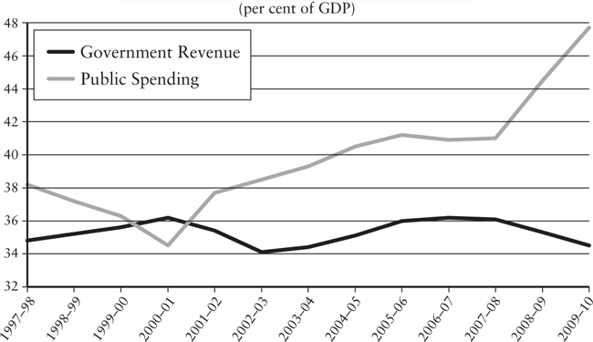
Gordon Brown was not an imprudent Chancellor. Between 1997–8 and 2006–7, the current account balance averaged 0.1%. Over the same period public sector net borrowing averaged 1.6%. With economic growth averaging 2.8% over the period, the national debt fell from 43.35% of GDP to 36.6%. Unemployment fell from 7% to 5%. Inflation averaged a little over 2% a year. This was a record of successful economic management. Brown could, and did, claim he had stuck to his fiscal rules.3
However, Brown’s claim was less robust than it seemed. First, the successful pre-crash current account outcome was achieved by redefining when cycles started and ended, and balancing early surpluses against later deficits. By 2006–7, with the current spending budget in deficit, maintaining the golden rule over the next cycle would have been ‘challenging’. Secondly, capital budget probity was being flattered by extensive use of the Private Finance Initiative (PFI) to build hospitals, schools and some expensive transport projects. PFI replaced spending financed by public debt with spending undertaken by private firms for which they were repaid by leasing agreements over periods of up to thirty years. It added nothing to the public debt, but gave rise to a higher stream of recurrent costs over the life of the asset than ordinary public procurement would have done. Its use allowed Brown to get a lot of capital spending ‘off budget’ and stick within the ‘prudent’ debt/GDP limit of 40 per cent.
The issue for macroeconomic policy is not whether PFI was a sleight of hand, but whether the investment it made possible would have taken place in its absence. A Keynesian would argue that, given the state of public opinion, PFI was the only way open to the government to drag private investment up to the level of full employment saving. It did this by converting uncertain into certain expectations for a large class of investments. In the absence of PFI, unemployment would have been higher and growth slower. PFI was as Keynesian as it was possible to be in a non-Keynesian world. The unfortunate effect of the deception, though, was to disguise the extent to which government procurement policy was actually propping up the British economy.
Figure 27. UK tax revenue and spending4

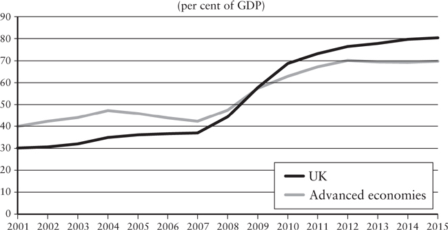
The economic downturn of 2008–9 caused a large deterioration in government fiscal positions and a rise in public debt to GDP ratios.
Advanced country governments acquired large deficits willy-nilly, as their revenues shrank and their spending on unemployment benefits rose. But there were also substantial discretionary responses: in Britain these included a temporary cut in VAT from 17.5 per cent to 15 per cent and accelerated capital spending. Rescuing the banks involved governments raising hundreds of billions in the bond markets, causing deficits to balloon: the rescue of the Royal Bank of Scotland alone cost £46 billion. Rescue operations included the co-ordinated $1 trillion stimulus measures agreed by the G20 in London in April 2009, with the British Prime Minister Gordon Brown taking the lead.5
The acute phase of the world crisis was over by the third quarter of 2009; however, a secondary Eurozone crisis was superimposed on the original one in 2010–11. Given the pre-crash orthodoxy, and a widespread misunderstanding of the public financing problem, it is not surprising that the fiscal brakes were slammed on. The fact that ‘Keynesian measures’ had averted a politically life-threatening collapse of the world economy was considered much less important than the unbalanced budgets governments were left with. Gordon Brown refused to be ‘another Philip Snowden’ (for the original one, see pp. 112–13). The trouble, explained his Chancellor, Alistair Darling, was the ‘Taliban wing’ of the Treasury who thought Snowden was right.8
Figure 28. Government budget deficits6
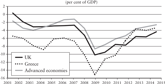
Figure 29. Government net debt7
The global turning point can be dated from the meeting of the G7’s finance ministers at Iqaluit in Canada in February 2010, which, dominated by the Greek crisis, committed governments to slashing deficits.9 Orthodox economists argued that cutting public spending would boost output by reducing borrowing costs and increasing confidence. In a pallid echo of Keynes’s ‘paradox of thrift’, the larger G20 acknowledged, in a declaration following its 2010 Toronto summit, that ‘synchronised financial adjustment [i.e. if all governments tried to reduce their deficits simultaneously] across several major economies could adversely impact the recovery’,10 but only President Obama stood out against the stampede towards what Germany’s Finance Minister Wolfgang Schäuble approvingly dubbed ‘expansionary fiscal consolidation’. Obama was supported by economists Paul Krugman, Joseph Stiglitz, Robert Shiller, Larry Summers, Nouriel Roubini and Brad DeLong. But ‘expansionary fiscal consolidation’ became the consensual view of Europe’s finance ministers.11 The majority of financial economists supinely followed the lead of the consolidators. Of the UK’s top economic journalists, Martin Wolf and Samuel Brittan of the Financial Times and Larry Elliott of the Guardian were lonely dissenters. This was at a time when global output was still 5 per cent below what it had been pre-crash.12 The British economics profession was largely silent.
This change of gear presumed that the recovery from the slump that had started in the third quarter of 2009 had gained strong independent momentum, and that fiscal consolidation was needed to maintain this momentum. In practice the shift to austerity in the UK and the Eurozone was followed by a marked slowdown in recovery, so much so that by mid-2010 most commentators were predicting a ‘double-dip’ recession or an L-shaped recovery. The truth was that the economies of the world were on life-support, and governments were switching the machines off.
Contrary to David Cameron’s rhetoric, UK public finances before the crash were not out of line with major comparators (see Figures 28 and 29). The real deterioration in the UK government’s position, as for all governments, took place because of the slump, the British economy contracting by about 7 per cent between the second quarter of 2008 and the third quarter of 2009.
Labour’s Chancellor of the Exchequer Alistair Darling announced a ‘fiscal consolidation plan’ in his pre-budget statement of autumn 2009. This committed the government to reducing the budget deficit, then projected to be 12.6 per cent of GDP in 2009–10, to 5.5 per cent by 2013–14, and to have net debt falling as a percentage of GDP by 2015–16.
Two letters that appeared in the British press early in 2010 give the flavour of the British debate. Twenty economists, headed by Tim Besley, wrote a letter to the Sunday Times on 4 February 2010, arguing that a faster pace for deficit reduction, especially on the spending side, was needed to sustain the recovery and restore confidence. Marcus Miller and Robert Skidelsky fronted a reply in the Financial Times on 18 February, arguing that the ‘timing of the measures should depend on the strength of the recovery’. Each letter got the support of a Nobel Prize-winner. The war of the economists had resumed. It has continued ever since.
Martin Wolf explained the state of opinion in mid-2010. The cutters emphasized that world economic recovery had been stronger than expected, that government deficits ‘crowd out’ private spending, and (if they were Austrian economists) that a deep slump was needed to purge past excesses. More moderate cutters argued that cutting the deficit would avoid a spike in borrowing costs, pointing to the peaking of Greek government debt at 12 per cent. Should fiscal tightening lead to the weakening of the recovery, monetary expansion (quantitative easing) was always available to offset it. The postponers emphasized the fragility of the recovery, its dependence on fiscal stimuli, and the existence of huge private sector surpluses. Wolf agreed with the postponers. ‘If anything, further loosening is needed.’13
Of key importance in swinging the debate in the UK over to the fiscal consolidators’ side was the political narrative spun by the Conservatives. As Chancellor of the Exchequer from 1997 until 2007, Gordon Brown had imprudently made ‘prudence’ his watchword. The Conservatives now milked the story of Brown’s fall from grace for maximum electoral impact. Reckless spending by the Labour government had not only contributed to the scale of Britain’s economic collapse, but had left Britain dangerously deep in debt. The Conservative narrative also protected the City of London by blaming the crisis on Labour.
A key point in this tale spun to deceive was that a large part of the post-crash deficit was not cyclical, but ‘structural’; that is, caused by government over-spending preceding and during the crash. Therefore, it was not sufficient to rely on the natural forces of recovery to eliminate the deficit: surgical operations were needed. And unless the government started on such operations immediately, belief in the government’s determination to restore budget balance would wither, causing confidence to flag and recovery to falter.
The Conservatives did not actually accuse the Labour government of having caused the world slump. Their charge was that, by breaking its own fiscal rules it had deprived itself of the ‘fiscal space’ to respond to the crisis by weakening confidence in government’s management of the public finances. A government, like any household threatened with mortgage foreclosure, should cut its spending as soon as possible: instead the Labour government had increased its spending. The government was unable to make a successful defence of its record and, in the general election of May 2010, lost power to a largely Conservative Coalition government, headed by Cameron. George Osborne became Chancellor of the Exchequer. In October 2008, Osborne had denounced the growing public deficit as a ‘cruise missile’ aimed at the heart of the British economy. As Chancellor, he was so vociferous about the dire straits to which Labour had reduced the public finances that people wondered whether he was inviting speculators to do a ‘bear’ on Britain.14
In his first budget, in June 2010, Osborne pointed to the consequences of failure to tackle the deficit:
Higher interest rates, more business failures, sharper rises in unemployment, and potentially even a catastrophic loss of confidence and the end of the recovery. We cannot let that happen. This Budget is needed to deal with our country’s debts. This Budget is needed to give confidence to our economy. This is the unavoidable Budget.
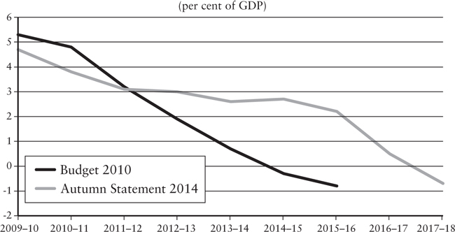
He announced tax increases and spending cuts, which, he claimed, would reduce the budget deficit (public sector net borrowing, PSNB) in a ‘single parliament’, i.e. by 2015, from 11 per cent of GDP to 1 per cent. Net debt would peak at 70 per cent of GDP before falling to 67.4 per cent in 2015–16. At the same, he specifically pledged to liquidate the ‘structural’ or ‘cyclically adjusted’ deficit’ (see below, p. 237), then estimated at 5.3 per cent of GDP, over the same period.* The measures he announced represented a fiscal policy tightening of 6 per cent of GDP. The Office for Budgetary Responsibility (OBR), the new Treasury watchdog he had set up, predicted that this would reduce the growth rate in the economy by only 0.4 per cent over the following two years.
Basing his policy on OBR forecasts, Osborne predicted that the British economy would grow 2.3% in 2011, 2.8% in 2012, and 2.9% in 2013.15 The fiscal forecast thus depended on the output forecast. Actual growth turned out to be 1.5% in 2011, 1.3% in 2012, and 1.9% in 2013, and Osborne had to borrow £40 billion more in 2010– 11 than he had anticipated because of the growth slowdown. In 2010, the OBR reckoned that the economy would grow by 17.2 per cent between 2010 and 2016; in fact it grew by 12.9 per cent (see p. 270). Such errors were bound to wreak havoc with the budget figures. PSNB was still over £50 billion in 2015–16: it is now expected to fall to £30 billion by 2021–2. Net debt (in November 2017) was now expected to peak at 88.8 per cent of GDP in 2017–18. Five-year targets, actual or rolling, have been abandoned. The ‘structural’ deficit has slowly come down, but this was because the economy eventually started growing faster than Osborne was able to cut spending. His cuts delayed the reduction of all the deficits, rather than expedited them.
So much for the record. Three questions may be asked. The first, and broadest, concerns the theory of fiscal policy in a slump. The second examines the confusions surrounding the notion of the ‘deficit’ and its financing. The third is about the effect of the slump on the long-term growth prospects of the economy.
Keynesians say that national output falls when there is an excess of planned saving over planned investment. Typically the private sector wants to save more than it wants to invest. To the extent that this creates an excess demand for bonds, the private sector’s excess saving will be exactly mirrored by an increase in the public sector’s ‘dissaving’ – more familiarly, by an increase in the budget deficit. If the government now tries to increase its own saving by cutting its spending, the result will be a fall in national income and output until the excess of saving over investment is eliminated by the community’s growing impoverishment.
Figure 30. Estimates of UK cyclically adjusted budget deficit16
An identical argument can be made in terms of output and income. If output falls below trend there is an ‘output gap’: the economy is producing less output than it could, there is spare capacity of plant and workers. If there is an output gap, an increase in loan-financed government investment will cause a multiplied increase in output. By the same token, a reduction in the deficit (fiscal consolidation) would cause the output gap to grow – spare capacity to increase by a multiple of the reduction.
The crucial mistake in Osborne’s austerity policy was to ignore the distinction between the numerator and denominator of the public debt fraction. He concentrated on cutting the numerator (the deficit) and ignored the effect of his policy on the size of the economy (the denominator).
Although Osborne no doubt had an ideological reason to slash the deficit, the technical mistake was that of his advisers. The OBR’s Fiscal and Economic Forecasts running from June 2010 largely ignore the impact of changes in government spending on national saving, investment, income and output. For example, the OBR Forecast of June 2010 (p. 33) said that the fiscal consolidation would have ‘no effect’ on output growth. In November 2011, the OBR acknowledged that falling government consumption and investment would reduce GDP growth slightly, but claimed that this would be ‘fully offset’ by looser monetary policy (p. 56). In December 2012 it was wondering why it had overestimated growth in the previous two years. Its answer was higher than expected inflation and weaker than expected investment (p. 27). By December 2013 it was admitting that ‘Fiscal consolidation is highly likely to have reduced growth in recent years’, other things being equal. However, with a budget deficit of 11 per cent of GDP ‘other things would almost certainly not have been equal’ (p. 53).
The OBR never attempted to update its pre-crash estimates of the fiscal multiplier. Its forecasting model, in other words, was a barely modified pre-crash model, in which fiscal multipliers were assumed to be close to zero because the economy was at full employment. This was despite the fact that the British economy had shrunk by almost 7 per cent between 2008 and 2009, from peak to trough of the crisis.
The OBR’s understanding of the economy was boosted by three academic arguments.
At the end of 2008, with output still falling, IMF forecasters spoke of a multiplier of between 0.3 and 0.8. What this meant was that fiscal expansion could not help the economy; even more importantly, that fiscal contraction would do it very little harm. Nothing better illustrates the orthodox pre-crash mindset that budget operations had no effect on the real economy. In March 2009, at the depth of the crisis, IMF staff reinforced the message that it was safe to start cutting deficits by estimating negative fiscal multipliers of between 0.3 and 0.5 for tax increases, and 0.3 and 1.8 for spending cuts. By 2013, IMF economists Olivier Blanchard and Daniel Leigh admitted they had got it wrong: fiscal multipliers had been ‘substantially above 1’.17 Their review of the evidence from twenty-six countries, entombed in tortuous econometrics and technical jargon, concluded that ‘the forecasters significantly underestimated the increase in unemployment and the decline in domestic demand associated with fiscal consolidation’. They found an ‘unexpected’ output loss of 1 per cent a year ‘for each 1 per cent of GDP consolidation’. Their models, they said, had let them down: ‘Under rational expectations, and assuming that the forecasters used the correct model, the coefficient on the fiscal consolidation forecast should be zero.’ This was as near as their prose allowed to admitting that they had been using the wrong model. But so had every other prominent forecasting organization. They were all wrong together. On such foundations was policy built and lives blighted.18
In 2010, the doctrine of ‘expansionary fiscal contraction’19 swept Europe’s finance ministries. Propounded by economists of the Bocconi School in Italy, it reversed the sign of the Keynesian multiplier by claiming that fiscal consolidation would cause output to grow by increasing confidence. The boost to confidence induced by a ‘credible programme of deficit reduction’ would stimulate enough extra demand to more than offset any adverse effects of fiscal contraction.
In April 2010, a leading proponent of this doctrine, Alberto Alesina, assured European finance ministers that ‘many even sharp reductions of budget deficits have been accompanied and immediately followed by sustained growth rather than recessions even in the very short run’.20 A key point in Alesina’s presentation was that spending cuts were much more effective than tax increases. Osborne took him at his word. In his consolidation plans, tax increases played a minor role; the emphasis was on spending cuts, especially cuts to welfare and public sector employment.
Following criticism of his methodology and findings by IMF and OECD staff, Alesina became considerably more circumspect. By November 2010 he was writing: ‘sometimes, not always, some fiscal adjustments based upon spending cuts are not associated with economic downturns’.21 But the damage had been done.
Since 2011 little has been heard of ‘expansionary fiscal contraction’. We got the contraction, but not the expansion.
Two American economists, Carmen Reinhart and Kenneth Rogoff, produced another correlation to bolster the austerity case. They attributed the ‘vast range of crises’ they had analysed to ‘excessive debt accumulation’.22 They noticed that, once the public debt–GDP ratio crashed through the 90 per cent barrier, ‘growth rates are roughly cut in half’.23 Early in 2013 researchers at the University of Massachusetts examined the data behind the Reinhart–Rogoff work and found that the results were partly driven by a spreadsheet error:
More importantly, the results weren’t at all robust: using standard statistical procedures rather than the rather odd approach Reinhart and Rogoff used, or adding a few more years of data, caused the 90% cliff to vanish. What was left was a modest negative correlation between debt and growth, and there was good reason to believe that in general slow growth causes high debt, not the other way around.24
Reinhart and Rogoff explained lamely that:
We do not pretend to argue that growth will be normal at 89% and subpar (about 1% lower) at 91% debt/GDP any more than a car crash is unlikely at 54mph and near certain at 56mph. However, mapping the theoretical notion of ‘vulnerability regions’ to bad outcomes by necessity involves defining thresholds, just as traffic signs in the US specify 55mph.25
It is hard to believe that even academics are so naïve as not to realize that politicians and journalists would seize on the actual speed limit rather than the ‘vulnerability regions’. George Osborne said that Reinhart and Rogoff were the two economists who influenced him most.26
It is important to understand why these economists got things wrong. Technical mistakes in data mining there may have been, but these were trivial. The reason they were wrong was that the forecasting models they were using led them to expect the results they got: fitting the data to the model was child’s play for a competent technician. These models were based on the neo-classical tool kit – rational expectations, optimizing agents, forward-looking consumers, unimpeded markets, equilibrium – which demonstrated the stability of economies at their natural rate of unemployment. The forecasters got what they expected and started scratching their heads only when real events proved them wrong.
The main features of the British Treasury’s position in 2010 reflected the mainstream forecasting models of the time:
1. Based on the Bank of England’s macroeconomic model, the Treasury forecast a V-shaped recovery, with economic growth bouncing back to about 3 per cent as early as 2011.27 They discounted the possibility of an L-shaped recovery and ‘underemployment equilibrium’. In short, they accepted the IMF’s position on the smallness of the fiscal multipliers.
2. With a strong economic recovery, gradual deficit reduction would not be contractionary: in fact it would keep the recovery going by giving confidence that public finances were being brought under control. Repairing the damage of the Brown Chancellorship loomed larger in the Osborne–Treasury mind than repairing the damage of the slump. In any case, any minor contractionary impact of fiscal tightening could be offset by monetary (quantitative) easing. These were the essentials of Alesina’s doctrine.
3. Confidence was especially important because of the worsening of the Eurozone debt crisis, especially that of Greece. So the Treasury argument was that, provided the government had a ‘credible’ deficit reduction plan, there would be no domestic obstacle to rapid and sustained recovery, but if it did not, it might well face a confidence-destroying fiscal crisis. In fact, Osborne argued that austerity would generate confidence, because it signalled the government was ‘living within its means’.
To explain the nugatory fiscal multipliers estimated by the IMF and others, three familiar items from the neo-classical repertoire were trotted out.
The American economist John Cochrane wrote: ‘If the government borrows a dollar from you, that is a dollar that you do not spend . . . Jobs created by stimulus spending are offset by jobs lost from the decline of private spending. We can build roads instead of factories, but fiscal stimulus can’t help us to build more of both.’28 This was the replay of the Treasury View of the 1920s. In his first budget, George Osborne talked about an overblown state ‘crowding out private endeavour’. Thus closely did policymaking track academic simplicities.
Ricardian equivalence: government borrowing is simply deferred taxation. Expecting to pay taxes, people would increase their savings. The increased savings would completely offset the extra government spending, leaving a multiplier of zero. Osborne actually referred to ‘Ricardian equivalence’ in his Mais Lecture of 2010.29
The government’s increasing demand for funds puts upward pressure on interest rates. The rise in interest rates will offset any stimulus afforded by the extra borrowing. This was a cogent argument for the Eurozone, where the European Central Bank was constitutionally debarred from buying government debt. However, it was untrue for the USA, the UK, China and Japan, whose central banks could be ordered or persuaded to buy gilts to offset any sign of a rise in longterm interest rates. This would enable the deficit to continue without financial crowding-out. In the extreme case (see Appendix 8.1, p. 246), the deficit can be entirely financed by advances from the central bank.
Figure 31. Cost of government borrowing
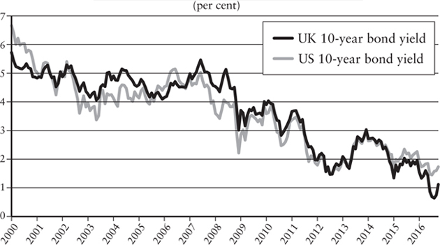
In practice, the UK Treasury was able to go on borrowing at very low rates of interest, mainly because the Bank of England was buying up government securities.
This was decisive for the Treasury. Greek government bond yields rose to 10 per cent in May 2010. As Besley and co. pointed out in their letter to the Sunday Times, the risk was that ‘in the absence of a credible deficit reduction programme’ there would be a ‘loss of confidence in the UK’s economic policy framework’. Agents with the correct model of the economy (i.e. Besley and co.’s model) would realize that a government which embarked on fiscal expansion was out of control. This would lead to a crisis of confidence, leading to an escalating cost of government debt as fear of default grew.30
The analogy with Greece was entirely misconceived, because the Greek government depended on the international bond markets; Britain’s did not. The further assumption that bond markets had the ‘correct’ model of the economy is ludicrous. In April 2010, they had ‘priced in’ a self-sustaining recovery. By July they were ‘pricing in’ a double-dip recession.31 They were the creators of the ‘noise’ on which their deals depended.
The Treasury’s arguments were different ways of saying there was no output gap and therefore no positive multiplier. They are contemporary versions of the Treasury View which Keynes fought against in 1929–31, and which he wrote the General Theory to refute; modern restatements of Say’s Law. Economics had come full circle.*
At the popular level, austerity policy was supported by a collection of such catchphrases as ‘The gravity train had to stop’ and ‘You can’t spend money you haven’t got’, which came much more readily to mind than more sophisticated Keynesian arguments. Two exhibits from the treasury of financial folklore resonated strongly with the public.
First, was the Swabian housewife. This mythical lady made her appearance on the world stage when German Chancellor Angela Merkel praised her in 2008 for her frugality, which, she implied, should be followed by business and governments. The latest version of this prudent housewife was produced by the British Chancellor of the Exchequer Philip Hammond in his spring budget statement of March 2018: ‘First you work out what you can afford. Then you decide what your priorities are. And then you allocate between them.’ This is good advice for households, but nonsense for governments. With its power to raise taxes, to borrow and re-borrow, and to print money indefinitely, the government’s budget constraint is much looser than that of the individual household.32
The second was the claim that the national debt was a ‘burden on future generations’. There are two fallacies in this. First, insofar as spending is financed by bonds, not taxes, this represents an intragenerational transfer between bond-holders and taxpayers at a single point in time.33 Secondly, if a government borrows from this generation to create assets for the use of future generations (as in the case of a long-gestating infrastructure programme) or, indeed, simply to avoid periods of ‘lost growth’, no net burden arises for any generation, present or future.
There was a more substantial public finance argument in favour of balancing the budget at full employment. This was that the public sector was bound to allocate capital less efficiently than the private sector. It was one thing to have the unemployed digging holes and filling them up again; another to replace private sector with public sector jobs. At full employment, efficiency issues replace demandmaintenance questions.
Having given full allowance for the attraction of orthodox rhetoric, it should not have been too difficult for competent politicians to get over the idea that ‘If no one’s buying cars there’s no point in making them’, or ‘If the government borrows money to build you a house, that’s a benefit both to you and your children’.
With the onset of the crisis the fiscal numbers worsened dramatically. Public sector net borrowing (PSNB) in 2009–10 was projected to be 11.2 per cent of GDP. The national debt was set to rise to 65 per cent of GDP in 2009–10 and to 75 per cent in 2013–14. It was the abrupt turnabout in the fiscal position that converted the story of Gordon Brown’s prudence into one of extravagance, clearing the ground for the consolidators. ‘Cutting the deficit’ became Osborne’s obsession. But which deficit was to be cut?
The basic concept for the deficit is public sector net borrowing. This is the raw, unadjusted difference between government receipts and expenditure. At any given rate of taxes and spending, PSNB rises automatically in a downturn as tax revenue falls and spending on unemployment increases; and it shrinks automatically in an upturn for the reverse reason, providing economies with a ‘built-in’ stabilizer. It can either be a plus number (meaning the budget is in deficit), a minus number (meaning a surplus) or zero (meaning balance).
But there is also a ‘structural’ or ‘cyclically adjusted’ deficit: the excess of government spending (both current and capital) over ‘normal’ revenue – the revenue it would expect to receive if the economy were normally employed. (CAB (Cyclically Adjusted Budget Balance) = BB (Budget Balance) – CC (Cyclical Component).) The OBR explains:
The size of the output gap . . . determines how much of the fiscal deficit at any one time is cyclical and how much is structural. In other words, how much will disappear automatically, as the recovery boosts revenues and reduces spending, and how much will be left when economic activity has returned to its full potential. The narrower the output gap, the larger the proportion of the deficit that is structural, and the less margin the Government will have against its fiscal target, which is set in structural terms.34
It was the ‘structural’ deficit, ‘the sticky bit’, which would remain after recovery that Osborne aimed to reduce to zero by 2015–16.
The structural deficit is a typical piece of new classical mythmaking. It reflected the prevailing orthodoxy that fiscal expansion cannot raise the ‘normal’ or ‘trend’ rate of growth of a market economy, but it can reduce it, by diverting resources to the less efficient public sector. In other words, it comes out of the ‘crowding-out’ stable of thought. From this point of view, structural deficits are especially vicious since, unlike the automatic deficits that arise from an economic downturn, they are deliberately predatory on the private sector. But for a Keynesian this is the reverse of the truth: the ‘normal’ level of economic activity set up as a benchmark by the new classical economist, against which to estimate the size of the structural deficit, may be severely sub-normal in terms of an economy’s productive potential; in which case the so-called ‘structural’ deficit is simply the deficit the government should ‘normally’ run to keep the economy fully employed. It is part of the state’s fiscal sustainability, not a derogation from it.
In November 2008, Gordon Brown’s Treasury estimated the structural budget deficit at 2.8 per cent for 2008–9. In June 2010, Osborne pledged to liquidate a structural budget deficit of 5.3 per cent for 2009–10. (See Figure 32 for IMF estimates.)
How had a cyclical downturn caused the estimate of the structural deficit to roughly double? The answer given by the Osborne Treasury was that the previous government had overestimated the ‘normal’ rate of growth of the British economy and therefore the revenues that would accrue from it:
Figure 32. Estimates of the UK structural deficit, pre- and post-crisis35
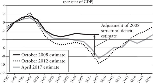
. . . a property boom and unsustainable profits and remuneration in the financial sector in the pre-crisis years drove rapid growth in tax receipts. The spending plans set out in the 2007 Comprehensive Spending Review were based on these unsustainable revenue streams. As tax receipts fell away during the crisis, the public sector was revealed to be living beyond its means.36
There is obviously some truth in this. The British economy had been growing in a lopsided way, with the financial sector ballooning while the rest of the private economy stagnated. Labour’s pact with the Mephistopheles of high finance ruined it in the end. But the tale of the structural deficit also reveals the flimsy nature of the macroeconomics on which policy was – and continues to be – based.
In a 1986 paper Olivier Blanchard and Larry Summers used the word hysteresis to describe a situation not when output falls relative to potential output, but when potential output itself falls as a result of a prolonged recession.37 What happens is that the recession itself shrinks productive capacity: the economy’s ability to produce output is impaired, on account of discouraged workers, lost skills, broken banks and missing investment in future productivity. That is, economic contraction and slow recovery can damage the supply-side of the economy, so recovery becomes a matter not of increasing demand but of rebuilding supply. In the post-recession years, the impact of hysteresis was felt not so much in the continuation of high unemployment but in the collapse of productivity, as workers were forced to move to lower productivity jobs.38
Marcus Miller and Katie Roberts have produced a stylized picture (Figure 33) of what may have happened in countries like the UK since 2008.
Instead of supply recovering to restore previous potential output, the economy resumes growth with a lower potential output. This matters for the structural deficit in the sense that lost productive capacity, and the concomitant reduced tax base and larger spending, turns deficits that previously were cyclical into deficits that are structural. With fewer people paying taxes when the economy returns to growth, the cyclical deficits will persist.
Figure 33. Hysteresis31
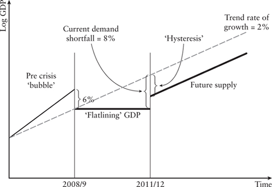
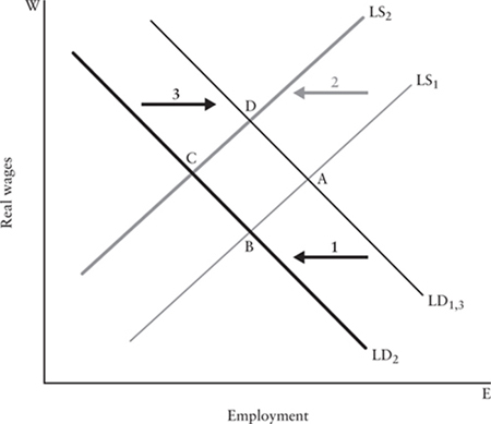
Figure 34 focuses on labour supply. In the first instance, demand for labour falls as a consequence of an external shock – for instance a banking crisis, as in 2008. This shifts the labour demand curve from LD1 to LD2 with the result that employment decreases from point A to B. Over time, the skills of those who have been made redundant by the fall in demand start to depreciate. This is represented in the shift in the labour supply curve from LS1 to LS2. Even with a resurgence in demand bringing back the curve from LD2 to LD3 the depreciation of skills has left the economy at a permanently lower level of employment, D.
The implication of hysteresis is that any policy which minimizes the period of recession minimizes the loss of potential output. It is a modern answer to the Treasury View.
Figure 34. Adjustment of labour supply in response to an external shock
The recovery patterns shown in Figure 35 are correlated with the intensity of austerity policies. Contrary to Alesina, the less austerity, the quicker the resumption of growth. The crucial years are 2011–12, when the US continued growing, the UK grew but at a weaker rate than the US, and the Eurozone went into a double-dip recession.
American policy was broadly Keynesian, despite anti-Keynesian rhetoric which was fiercer than anywhere else, except Germany. Fiscal austerity only really started in 2013 when Congress forced spending cuts on the Obama Administration. By then, however, the economy had recovered its lost output. The Bush Administration produced the $152 billion Economic Stimulus Act of 2008, a large part of which consisted of $600 tax rebates to low- and middle-income households. In early 2009 President Barack Obama signed the American Recovery and Reinvestment Act. This mandated the government to inject $831 billion (originally $787 billion) into the US economy over the decade 2009–19. Most of this was spent in 2009 and 2010. In July 2010, a report of the President’s Council of Economic Advisers claimed that the stimulus had saved or created 2.5–3.6 million jobs, and had caused US GDP to be 2.7–3.2 per cent higher than it would have been without the stimulus. This was in line with the projections by the non-partisan Congressional Office of the Budget.41 Fiscal expansion was accompanied by monetary easing in the form of quantitative easing (QE). The US performance was not especially robust: the proportion of working-age adults in work fell from 72 to 67 per cent, income inequality widened, productivity fell. But it was much better than in Britain and Europe. It showed that Keynesian policy worked.42
Figure 35. Post-crash outcomes: UK, USA and Eurozone40
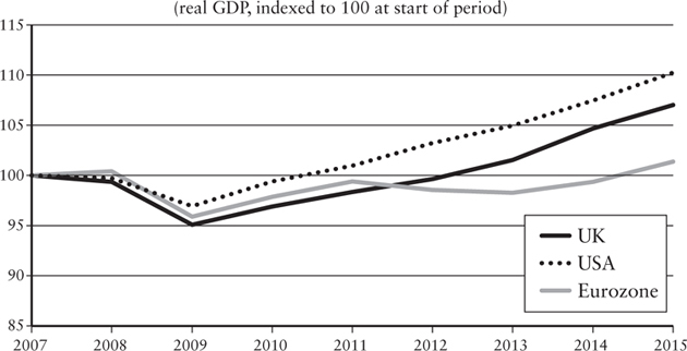
The Eurozone has had the worst record, partly because EU fiscal rules mandated balanced budgets, mainly because austerity was imposed on Eurozone governments as a condition of loans from the ECB and IMF. Italy, Portugal, Spain and Greece all experienced double-dip recessions. A recent study estimates that cumulative output losses due to fiscal austerity in the euro area between 2011 and 2013 range from 5.5 per cent to 8.4 per cent of GDP, depending on estimates of the multiplier.43 Greece is the worst example; the country was set up to fail by a troika of creditors, which forced it to implement impossibly stringent austerity policies in order to receive additional loans, its GDP, in consequence, falling by 27 per cent. The euro crisis was only finally overcome in 2013–14.44
The UK is an intermediate case. The British government was not forced into austerity, it chose it. The main impact of austerity was felt in 2011–12. In late 2010, George Osborne was proclaiming that the economy was ‘on course’ and that Britain was ‘on the mend’.45 The economy promptly proceeded to flat-line for two years. Osborne later admitted that he had got himself ‘into a sort of hole: shut in my room, didn’t go out’.46 The stagnation forced a rethink. The fiscal consolidation targets were pushed outward in time; further monetary measures came in the form of a second (and then third) bout of monetary easing, and the Treasury started to subsidize crippled bank lending. The economy slowly mended as the austerity was relaxed.
Jordà and Taylor presented a ‘counterfactual analysis’ of Coalition austerity in the UK during the Great Recession. Their analysis of what would have happened to the patient had he not taken the medicine (austerity) is shown in Figure 37.
Figure 36. Post-crash outcomes: Germany, Greece and Eurozone47
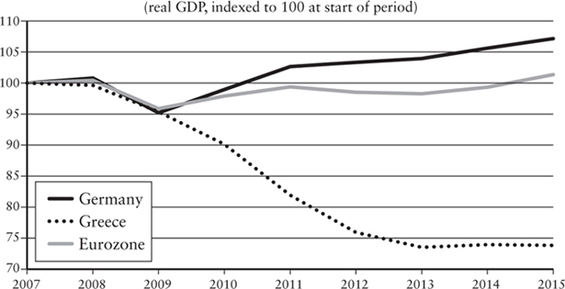
Figure 37. UK austerity – counterfactual medicine48
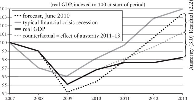
Simon Wren-Lewis of Oxford University calculates the cost of austerity up to 2017 as between £4,000 and £13,000 per household.49 As for workers, the situation was worse still. Ninety per cent of the population have not had a pay rise for ten years, and household debt is back to its pre-crash level.
One might be tempted to conclude that the debate between the Keynesians and the Osbornians, like the confrontation between Keynes and Sir Richard Hopkins before the Macmillan Committee in 1930, resulted in no clear-cut victory for either side. Osborne could (and did) argue that GDP had recovered to its pre-crash level by 2013–14, that Britain now had full employment, and that the public finances were relatively sound. In other words, the Keynesian contention that, in the absence of a stimulus, the British economy was bound to remain in semi-slump, had no foundation. Automatic recovery forces and the confidence-raising effects of austerity were enough to lift the economy out of slump territory. In different words, there were no multipliers to be had from fiscal stimuli.
However, this conclusion would be wrong, for three reasons. First, it does not acknowledge that the return to growth in mid-2009 was not ‘automatic’, but was the result of the Keynesian measures taken in Britain and elsewhere to stimulate the economy. The reversal of these measures in Britain did not ‘restore’ growth; it was accompanied by a reduction in growth by an estimated 1 per cent a year between 2010 and 2015.50
Secondly, all competent authorities agree that fiscal contraction delayed recovery, slowed down growth and destroyed growth potential. Headline unemployment in Britain has fallen to just under 5 per cent, the lowest since 1975, but this excludes the millions of part-time workers who say they would work full-time if they could, those forced into precarious self-employment and on to zero-hour contracts, and those over-qualified for the jobs they do. The vaunted flexible labour market revealed by the recession has delivered a sizeable ‘jobs gap’. If we take just two categories – those claiming unemployment benefit and those of the employed who say they would work longer hours if such work was available – about 11 per cent of the British workforce is ‘under-employed’.51 The opportunity to use available labour and cheap borrowing costs to build infrastructure was ignored: only 105,000 houses were built in Britain in 2011, the lowest number since the 1920s.
Thirdly, fiscal austerity was partly offset by monetary expansion and a fall in the sterling exchange rate. This is in line with the view that fiscal contraction in a recession need not cause a decline in aggregate demand, if there are offsetting forces of demand expansion. Still, the stagnation of 2010–12 suggests that the theory linking fiscal tightening to recovery is wrong. It was based on the careless view that a reduction in public spending is the same thing as a reduction in the deficit. But if the reduction in public spending reduces the growth rate, as is now generally acknowledged, it simultaneously reduces government revenues. This simple fact explains the disappointing progress towards deficit reduction.
In reality, the only deficits the deficit-hawks really mind about are deficits incurred to protect the poor. The wealthy have never been against tax cuts for themselves, even if this widens the deficit; and their economist friends have been busy demonstrating what wonderful multipliers are available for the economy if governments take this course. To cut the deficit for the poor and expand it for the rich – what more could one ask of government fiscal policy?52
A government with its own central bank does not have to raise money from the public to pay for its spending. It can simply order the central bank to print the money on its behalf. It incurs a liability to ‘its’ bank but not to anyone else; and its debt to its own bank never has to be paid back – a debtor’s dream! To limit this unique privilege of printing money, the convention (and in some cases legal requirement) has grown up that government spending has to be covered by taxation or borrowing from the public (considered deferred taxation). ‘Monetary financing’ of the deficit is advocated as a ‘last resort’ policy only for a ‘worst-case scenario’, when orthodox fiscal expansion to counter a recession is disabled by fears of rising debt.53
Technically, the central bank credits the Treasury with, say £50 billion, or alternatively the Treasury can issue £50 billion worth of debt, which the central bank agrees to hold indefinitely, rebating any interest received to the Treasury. The advantage of such financing is that it will raise aggregate demand without enlarging the national debt – the money the government owes to its holders. (For it to have its full effect, the increase in the money supply must be seen as permanent.) But, as Adair Turner writes: ‘[I]t is also clear that great political risks are created if we accept that monetary finance is a feasible policy option: since once we recognise that it is feasible, and remove any legal or conventional impediments to its use, political dynamics may lead to its excessive use.’ More succinctly, Ann Pettifor put it thus: ‘It is the bond market that keeps governments . . . honest.’54
It follows that I do not agree with modern monetary theorists that, because the government creates the money it spends, it is freed from the budget constraint faced by the individual firm or household. It is, of course, true that if the government spent no money, there would be no taxes. (But then there would be no government either!) But it does not follow that the money it spends automatically returns to it as tax revenue. As Anwar Shaikh rightly notes: ‘There is no such thing as a money of no escape.’55 The value of modern monetary theory is not in trying to prove that government can issue debt without limit, but in emphasizing that the ‘bonds of revenue’ are far looser than the deficit hawks claim.
* Osborne left himself some room for manoeuvre by making these five-year ‘rolling targets’, leaving it for the OBR to judge whether he was ‘on course’ at the start of any five-year period.
* As far as I can tell, the idea of bringing idle resources into use by means of the balanced-budget multiplier was never considered by policymakers. The government increases its expenditures (G), balancing it by an increase in taxes (T). Since only part of the taxed money would have actually been spent, the change in consumption expenditure will be smaller than the change in taxes. Therefore the money which would have been saved by households is injected by the government into the economy, itself becoming part of the multiplier process. The multiplier is greater still in a progressive tax system, since the rich save a greater proportion of their incomes than the poor. For advocacy of this policy, see Stiglitz (2014).