5Generalizations of the Lambert function

DOI: 10.1201/9781003168102-5

The Lambert function has surprisingly many applications in different areas of science. Still, there are problems that need functions that are more general than W. In this chapter we introduce some functions which are mainly studied in the literature because of their utility in applications.

5.1 The generalized Lambert function

5.1.1 The polynomial-exponential and rational-exponential type equations

Thinking on generalizations of the equation

zez=w,

we observe that the factor z on the left-hand side is a polynomial, albeit among the simplest ones. It would make sense to put a polynomial p(z) in place of z. Thus we arrive at an equation

p(z)ez=w.

Such an equation is named polynomial-exponential type. Another extension is when, in place of p(z), we put a rational function. A rational function is a fraction of two polynomials. We therefore write the extension as

p(z)q(z)ez=w.(5.1)

We refer to such an equations as rational-exponential type.

Notice that a Lambert-like equation with “additive polynomial part” would not result in a new problem. Take the equation

ez+p(z)=w.

This can very easily be transformed into a polynomial-exponential type:

ez+p(z)=w⇒ez=w−p(z)⇒1q(z)ez=1,

where

q(z)=w−p(z)

is a polynomial.

To reach the ultimate extension that we encounter in the literature, we put a polynomial r(z) in place of the simple polynomial inside the exponential function.

p(z)q(z)er(z)=w.(5.2)

All of these extensions are not mere generalizations for their own sake; equations of the form (5.2) are used in applications as we shall see the in Part III of this book.

5.1.2 The definition of the generalized Lambert function

If we factor the polynomials p and q (which can always be done over the complex plane), the rational-exponential type equation (5.1) becomes

(z−t1)(z−t2)⋯(z−tn)(z−s1)(z−s2)⋯(z−sm)ez=w.(5.3)

The solutions of this equation will be given by the branches of the generalized Lambert function. We introduce the notation

Wt1,t2,…,tns1,s2,…,sm;w(5.4)

for the solutions of equation (5.3).

We call the t_i parameters upper parameters, the s_js are the lower parameters. If there is no p or q, we do not write indices in the corresponding places. For example, the solutions of

p(z)er(z)=w

are written in the form

Wt1,t2,…,tn;w

provided that p(z)=(z−t1)(z−t2)⋯(z−tn).

It will be useful to set the type of equation (5.3) and of function (5.4) to be (n,m). Thus, instead of writing the lengthier generalized Lambert W function, we will often write Lambert function or W function of type (n,m).

In this generality, not much is known about the (5.4) function. We first see the cases when n and m are one or absent. Then we turn to the equation of type (1,1) because this case is fully understood.

5.1.3 Simple cases

Let us first study the simplest versions of the generalized Lambert function. If there are no polynomials at all in (5.3), we get the equation ez=w, so

W;w=log⁡(w).

This shows that the logarithm is a particular case of the generalized Lambert function.

Now let us see what happens if there is one upper parameter and there is no lower parameter. That is, we want to solve the equation

(z−t)ez=w.

We make the substitution

z−t=y (z=t+y),

and the equation becomes

yet+y=w, or, equivalently yey=we−t.

This is solvable in terms of the classical Lambert function, thus we get that

y=W(we−t),

and then

z=t+W(we−t).

We therefore get that

Wt;w=t+W(we−t).

In particular,

W0;w=W(w).

It is similarly easy to see that the Lambert function of type (0,1) is again the classical Lambert function:

 Ws;w=s−W−esw.

The complication comes when we have more parameters. But before going to investigate these cases, we remark some simple transformation formulas for the generalized W function.

5.2 Transformations of rational-exponential type equations

It is clear that we can permute the upper parameters and lower parameters among themselves; no change is made in the equation:

Wt1,t2,…,tns1,s2,…,sm;w=Wti1,ti2,…,tinsj1,sj2,…,sjm;w,

where i1,…,in and j1,…,jm are arbitrary permutations of the first n and m positive integers, respectively.

It is similarly obvious, that equal upper and lower parameters can be deleted:

Wt,t2,…,tnt,s2,…,sm;w=Wt2,…,tns2,…,sm;w.

Another, less trivial transformation is the following for w≠0:

Wt1,t2,…,tns1,s2,…,sm;w=−W−s1,−s2,…,−sm−t1,−t2,…,−tn;(−1)m+nw.(5.5)

The n=m=1 particular case is

Wts;w=−W−s−t;1w.

The proof of (5.5) is as follows. We start with (5.3), and take the reciprocal of both sides:

(z−s1)(z−s2)⋯(z−sm)(z−t1)(z−t2)⋯(z−tn)e−z=1w.

We now make the substitution

−z=y,(5.6)

so the last displayed equation transforms into

(−y−s1)(−y−s2)⋯(−y−sm)(−y−t1)(−y−t2)⋯(−y−tn)ey=1w,

which is equivalent to

(y+s1)(y+s2)⋯(y+sm)(y+t1)(y+t2)⋯(y+tn)ey=(−1)m+nw.

For this latter equation, the solution is

W−s1,−s2,…,−sm−t1,−t2,…,−tn;(−1)m+nw.

We still need to multiply this by minus one because of the substitution (5.6). After this step, one arrives at the right-hand-side of (5.5).

5.3 The (1,1) -type function and the r-Lambert function

The first case when the generalized Lambert function gives rise to a new function is when we have at least one upper and at least one lower parameter. We now study the (1,1) -type function Wts;w, and point out that we can incorporate t and s into one parameter which will be denoted by r. The arising function will be called the r-Lambert function.

Let us do the substitution

y=z−t

in the equation

z−tz−sez=w,(5.7)

for which the solution, by definition, is

z=Wts;w.

We get that

yy+t−sey+t=w,

or

yy−(s−t)ey=e−tw.

Multiplying by y−(s−t), a simple rearrangement gives the equation

yey−e−twy=e−tw(t−s).

Introducing the variable

r=−e−tw,

it comes that the last equation is the same as

yey+ry=r(s−t).

Set

u=r(s−t),

we finally get the equation

yey+ry=u.(5.8)

Notice that although u depends on r, s and t are arbitrary, so u can be considered as a variable independent of r. We therefore infer that equation (5.7) with two free parameters, and (5.8) with one free parameter are equivalent. For the solution(s) of the latter, we introduce the r-Lambert function, that is,

y=Wr(u).

In other words, the r-Lambert function at the point u is a real or complex number which satisfies the equation

Wr(u)eWr(u)+rWr(u)=u.

Remember that the solution z of (5.7) equals y+t, hence, by plugging in the original values of r and u, we arrive at the correspondence between the (1,1) -type function Wts;w=y+t=z and the r-Lambert function:

Wts;w=t+W−e−twe−t(t−s)w.(5.9)

This correspondence was first observed in [132]. It is now seen that it is enough to study the r-Lambert function which has only one parameter instead of the two-parameter Wts;w function.

The following chapter will be dedicated to the study of the r-Lambert function.

5.4 A series representation for the (1,1) -type function

The Taylor series of Wts;w around w=0 is an interesting one:

Wts;w=t−T∑n=1∞Ln′(nT)ne−ntwn,(5.10)

where T=t−s≠0, and Ln′ is the derivative of the nth Laguerre polynomialL_n. These polynomials can be defined via a Rodrigues-type formula:

Ln(α)(x)=x−αexn!dndxn(e−xxn+α).(5.11)

(In fact, these are the so-called generalized Laguerre polynomials; the classical ones are those with α=0.)

The proof of (5.10)

We use the Lagrange Inversion Theorem (1.51). Let

f(x)=exx−tx−s.

We choose a point in which f is zero, and then we invert its series in this point. This point is t. Hence, by Lagrange's theorem,

Wts;w=t+∑n=1∞wnn!lim⁡τ→tdn−1dτn−1τ−tf(τ)n.(5.12)

Here the only difficulty is the expression

lim⁡τ→tdn−1dτn−1τ−tf(τ)=lim⁡τ→tdn−1dτn−1τ−seτ.(5.13)

Recalling the Rodrigues formula (5.11), it can be seen that a modification of (5.13) will lead to a (generalized) Laguerre polynomial. Let us make this precise. The limit (5.13), if we expand it entirely, takes the form

e−nt∑k=1nAn,k(−1)k−1Tk.(5.14)

Here T=t−s.

We are now going to determine the coefficients An,k. An easy calculation gives the following table:

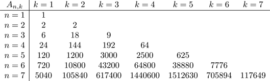
These numbers cannot directly be found in the OEIS [4] but the row sum appears under the identification number A052885. There we can find that A052885 equals the sum of

(n−1)!nk−1nk1(k−1)!.

Hence we can suspect that this is exactly what we are looking for,

An,k=(n−1)!nk−1nk1(k−1)!.

Once we have this conjecture, the proof is easy (by induction). Hence we can step forward, substituting this into (5.12):

Wts;w=t+∑n=1∞(we−t)nn∑k=1n(−n)k−1(k−1)!nkTk=

Wts;w=t−∑n=1∞(we−t)nn2∑k=1nnk(−nT)k(k−1)!.

Recalling the explicit expression for the generalized Laguerre polynomials [167, p. 775, Table 22.3]:

Ln(α)=∑k=0nn+αn−k(−x)kk!,

we can easily see that our inner sum in the Taylor series is simply

∑k=1nnk(−nT)k(k−1)!=−nTLn−1(1)(nT).

The relation [167, p. 778]

Ln−1(1)(x)=−Ln′(x),

finalizes the proof. Note that T≠0 is necessary in the above argument, especially in (5.14). T=0 stands for the standard log function. The proof is finished.

Further notes

1. The origin of the generalized Lambert function. According to our knowledge, it was a 2006 paper [162], where the idea of the generalization of the Lambert equation xex=a to (5.3) first emerged. It was observed in [162] that a molecular physics problem [160] and the general relativistic two-body problem [122] both need the same generalization of W, which is, using our terminology, the (2,0) -type Lambert W function.

2. Quaternionic Lambert equation and Matrix Lambert equation. The equation qeq=r where q and r are quaternions was studied in [65]. Equations of the form Sexp⁡(S)=A, where S and A are matrices were studied in [38, 189], for example.

3. Quadratic Lambert function. Equations of the form zeaz2+z=w and their applications to general relativity are studied in [133].

4. The discrete Lambert map and r-Lambert map. The equation xex=a can be studied over finite fields as well – in this case e must obviously be replaced with a primitive rootg, and equality becomes congruence: xgx≡a mod⁡pe is the discrete Lambert congruence, and xgx is the discrete Lambert map. This equation was extensively studied in [33, 117, 120, 190, 191]. The discrete r-Lambert map xgx+rx over finite fields was studied in [126].

5. The p-adic Lambert function. The p-adic Lambert function can formally be defined via the Taylor series for the principal branch. Some basic properties of the p-adic Lambert function were given in [127].

   See the web page of the author of this book for more information and up-to-date citations to newer papers on W and on its generalizations.

6. Problems. The general theory of the type (n,m) Lambert function might be elusive, but the next step after the well-known (1,1) -type function (or, equivalently, the r-Lambert function) might be a good starting point. So one can ask for the (2,0), (2,1), and (2,2) type Lambert functions' branch structure, Riemann surface, asymptotics, and other properties.

   Another problem to study is the branch structure, Riemann surface, and asymptotics of the above-mentioned quadratic Lambert function.