, in excess of the risk-free rate, Rf, on the excess return of the market,
  :
:Evaluating Trading Strategies
Performance Measures
Let us first consider some simple measures that can be used to evaluate a hedge fund’s overall performance or a specific strategy that the hedge fund has been using. Furthermore, these measures can be used to evaluate a strategy that a hedge fund is considering and has been simulating via a backtest, as discussed in the next chapter.
2.1. ALPHA AND BETA
The most basic measure of trading performance is, of course, the return, Rt, in a given period, t. The return is often separated into its alpha and beta. Beta is the strategy’s market exposure, while alpha is the excess return after accounting for performance due to market movements. Alpha and beta are computed by running a regression of the strategy’s return, , in excess of the risk-free rate, Rf, on the excess return of the market, :
![]()
Here, β (beta) measures the strategy’s tendency to follow the market. For example, suppose that β = 0.5. This means that if the market goes up by 10%, this strategy goes up by 0.5 × 10% = 5%, everything else being equal. For instance, if you invest half of your money in the stock market and the other half in cash, then your overall portfolio has a β of 0.5. In that case, your excess return will literally be 5% when the market goes up by 10%. More generally, your performance also depends on your idiosyncratic risk, measured by εt. For instance, if you only invest in biotech stocks rather than the overall market, then εt is the relative outperformance of your biotech stocks vis-à-vis the market. The idiosyncratic risk can be positive or negative, is zero on average, and is independent of market moves.
Knowing a strategy’s beta is useful for many reasons. For instance, if you mix a hedge fund with other investments, the beta risk is not diversified away, while idiosyncratic risk largely is. Furthermore, market exposure (“beta risk”) is easy to obtain at very low fees, for example, by buying index funds, exchange traded funds (ETFs), or futures contracts. Hence, you should not be paying high fees for market exposure.
Many hedge funds are (or claim to be) market neutral. This important concept means that the hedge fund’s performance does not depend on whether the stock market is moving up or down. That is, the hedge fund has equally good potential to make money in bull and bear markets because its strategy is not simply to bet on the market going up. Mathematically, being market neutral means that β = 0.
Another use of beta is that it tells us how to make a strategy market neutral. Indeed, even if a strategy is not market neutral, we can make it market neutral by hedging out the market exposure, and β gives us the hedge ratio. Specifically, for every dollar of exposure to the hedge fund strategy, we need to short β dollars of the market. The performance of the market-neutralized strategy is then
![]()
Since the idiosyncratic risk εt is zero on average, the expected excess return of the market-neutral strategy is
![]()
We see that the expected return in excess of the risk-free rate and the exposure to the market is given by the alpha, α. Alpha is clearly the sexiest term in the regression: It is the Holy Grail all active managers seek. Alpha measures the strategy’s value added above and beyond the market exposure due to the hedge fund’s trading skill (or luck, given that alpha is estimated based on realized returns).
If a hedge fund has a beta of zero (i.e., a market-neutral hedge fund) and an alpha of 6% per year, this means that the hedge fund is expected to make the risk-free return plus 6% per year. For instance, if the risk-free rate is 2% per year, the hedge fund is expected to make 8%, but the actual realization could be far above or below that, depending on the realized idiosyncratic shock.
The classic capital asset pricing model (CAPM) states that the expected return on any security or any portfolio is determined solely by the systematic risk, beta. In other words, CAPM predicts that alpha is equal to zero for any investment. Therefore, a hedge fund’s search for alpha is a quest to defy the CAPM, to earn higher returns than simple compensation for systematic risk.
A hedge fund’s true alpha and beta are estimated with significant error. Hence, if a hedge fund has an estimated alpha of 6%, how do we know whether this is luck or skill? To address this issue, researchers often look at the t-statistic, namely the alpha divided by the standard error of its estimate (an output of all regression analysis tools). A large t-statistic means that the alpha is large and reliably estimated, essentially because you have a long track record. Specifically, a t-statistic above 2 means that the alpha is statistically significant from zero, i.e., evidence of skill that defies the CAPM (although there can still be false positives and biases, e.g., if a manager shows only her best performing fund). A t-statistic smaller than 2 corresponds to an alpha estimate which is so noisy that it might have been achieved through luck.
We can also compute a strategy’s excess return above and beyond several risk exposures, not just the market risk exposure. For instance, academics often consider the following three-factor regression model due to Fama and French (1993):
![]()
where RHML is the return on a value strategy and RSMB is the return on a size strategy. Specifically, the high-minus-low factor (HML) goes long on stocks with a high book-to-market ratio (B/M) and shorts stocks with a low B/M. Similarly, the small-minus-big factor (SMB) goes long in small stocks and shorts big stocks. Therefore, βHML measures the strategy’s tendency to be tilted toward stocks with a high B/M (i.e., stocks that look cheap on this metric) and βSMB measures the tilt toward small stocks. Hence, the alpha in the three-factor regression measures the excess return adjusted for market risk, value risk, and size risk. Said differently, this alpha measures the hedge fund’s trading skills beyond simply taking stock market risk and tilting toward small-value stocks (which tend to outperform other stocks, on average).
2.2. RISK–REWARD RATIOS
As we have seen, a positive alpha is good while a negative alpha is bad. However, is a high positive alpha always better than a low positive alpha? Not necessarily. First, while alpha tells you the size of the market-neutral returns that a strategy delivers, it does not say at what risk. Second, alpha depends on how a strategy is scaled; for instance, a twice-leveraged strategy has twice the alpha of an unleveraged version of the same strategy. However, the quality of the strategy is what it is, so the performance measure should arguably be the same in both cases.
Risk–reward ratios resolve these issues. At a basic level, potential investors in a hedge fund want to know how the future expected excess return E(R – Rf) compares to the risk that the hedge fund is taking. The Sharpe ratio (SR) is a measure of just that and is also called the risk-adjusted return. It measures the investment “reward” per unit of risk:
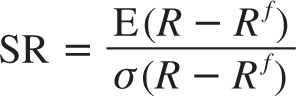
The investment reward is simply the expected excess return over the risk-free rate, that is, how much better did you do relative to putting your money in the bank? The risk is measured as the standard deviation σ (also called volatility) of your excess return. I describe below how to estimate these. Clearly, investors prefer higher SRs, as they prefer higher returns and lower risk (but their preferences might be more complex than what is captured by the Sharpe ratio when hedge funds have skewed returns and crash risk).
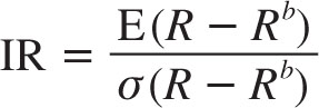
The SR gives the hedge fund credit for all excess returns, but we learned above that there is a difference between alpha returns and simple market exposure. The information ratio (IR) addresses this by focusing on the risk-adjusted abnormal return or, said differently, the risk-adjusted alpha:
![]()
The alpha and idiosyncratic risk ε come from a regression of the hedge fund’s excess return on some benchmark with excess return  :
:
![]()
If the hedge fund has a mandate to beat a specific benchmark, then the IR is often computed without running a regression. In this case, the IR is computed simply as the expected return in excess of the benchmark, relative to the volatility of this outperformance1:
Hence, the IR measures the extent to which the strategy beats the benchmark per unit of tracking error risk. Tracking error is the difference between the strategy’s and the benchmark’s returns, and tracking error risk is the standard deviation of this difference. Many hedge funds consider their benchmark to be physical cash (money in the mattress, i.e., Rb = 0), so they report the IR simply as
![]()
which is always higher than the SR, since it does not subtract the risk-free rate. Even if many hedge funds report this number, I view it as an unreasonable number as it gives the hedge fund credit for earning the risk-free rate (and depends on the level of interest rates). The IR is almost always reported as an annualized number, as discussed further below.
Both the SR and the IR are ways of calculating risk-adjusted returns, but some traders and investors say,
You can’t eat risk-adjusted returns.
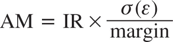
Suppose, for instance, that a hedge fund beats the risk-free rate by 3% at a tiny risk of 2%, realizing an excellent SR of 1.5. Some investors might say, “Well, it’s still just 3%. I was hoping for more return.” Whether this is a fair criticism or not depends on several things. First, it depends on whether the strategy’s risk really is that low on a long-term basis or this period was just lucky not to have a blowup (e.g., if the hedge fund is selling out-the-money options collecting small premiums until a big market move blows it up). If we suppose that risk really is low, then the question is whether one can apply leverage to the strategy to achieve a higher return and risk. With leverage, you can eat risk-adjusted returns. One way to apply “leverage” is to have the investor put more money in the hedge fund, but many investors prefer not to have a large notional exposure and need ready cash. Therefore, the question is whether the hedge fund can apply leverage internally. The answer to this question is given by the alpha-to-margin (AM) ratio (suggested by Gârleanu and Pedersen 2011):
![]()
The idea behind this ratio is to compute the return on a maximally leveraged version of a market-neutral strategy. To understand the AM ratio, note that while hedge funds can apply leverage to any strategy, there is a limit to this leverage, since hedge funds are subject to margin requirements, as discussed further in section 5.8. The maximum leverage that can be applied to a strategy is 1/margin. For instance, if the margin requirement is 10%, a hedge fund can get 10-to-1 leverage, and, in this case, the AM ratio is 10 times the expected market-neutral return. To be even more specific, if alpha is 3% per year, then the AM ratio is 30%. This means that if a hedge fund takes $100 of its capital, applies 10-to-1 leverage, and invests $1,000 in the strategy, then it has an alpha of 3% × $1,000 = $30, which is 30% of its $100 capital. The hedge fund may prefer this strategy to one trading illiquid securities that cannot be leveraged at all (margin is 100%) with an alpha of 7%. This alternative strategy has a lower AM ratio of 7%, despite its higher alpha. The AM ratio can be seen as the investment management equivalent of the return of equity (ROE) measure from corporate finance.
There is a close link between the AM ratio and the IR. The AM ratio is the reward per unit of risk (IR) multiplied by the extent to which the strategy can be leveraged, namely the risk per unit of margin equity:
If a hedge fund strategy has a significant crash risk, volatility may not be the best risk measure. To capture crash risk, the denominator is modified in performance measures such as the risk-adjusted return on capital (RAROC):
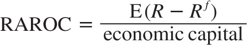
where economic capital is the amount of capital that you need to set aside to sustain worst-case losses on the strategy with a certain confidence. Hence, the denominator is the crash risk instead of day-to-day swings. Economic capital can be estimated using value-at-risk (VaR) or stress tests, concepts that we discuss in detail in section 4.2 on risk management. The Sortino ratio (S) uses downside risk:
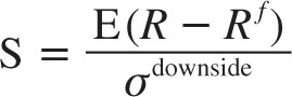
The downside risk (or downside deviation) is calculated as the standard deviation of returns truncated above some minimum acceptable return (MAR):
![]()
The MAR is often set to be the risk-free rate or zero. The indicator function in the calculation of downside risk, 1{R < MAR}, is the number 1 if the return is less than the MAR, and zero otherwise. Hence, the downside risk is not affected by how returns vary when they are above the MAR. Implicitly, this result is based on an assumption that investors care only (or mostly) about the downside. Therefore, the Sortino ratio assumes that investors do not care whether they make 5% in each of two years versus 1% the first year and 9% the next. In contrast, the SR is based on an assumption that investors prefer the former.
2.3. ESTIMATING PERFORMANCE MEASURES
To estimate expected returns, standard deviations, and regressions, we can use standard methods. Expected returns are estimated as the realized average return, using the available data over T time periods. Some people use geometric averages,2
![]()
while others use arithmetic ones,
![]()
The geometric average corresponds to the experience of a buy-and-hold investor who neither adds capital nor takes capital out of a hedge fund. The arithmetic average is the optimal estimator from a statistical point of view, and it corresponds more closely to the experience of an investor who adds and redeems capital in order to keep a constant dollar exposure to the hedge fund, under certain conditions. Whether using geometric or arithmetic averages, it is important to keep in mind that any estimate of future expected returns is extremely noisy. The precision of the estimate increases with the length of the sample period, but it is difficult to estimate expected returns, even with many years of data.
The standard deviation σ can often be estimated with more precision: It is the square root of the variance σ2, which is estimated as the squared deviations around the arithmetic average, 
![]()
2.4. TIME HORIZONS AND ANNUALIZING PERFORMANCE MEASURES
Performance measures depend on the horizon over which they are measured. For instance, table 2.1 shows that a strategy that has an annual Sharpe ratio of 1 has very different Sharpe ratios if measured over other time horizons, such as a Sharpe ratio of 2 over a four-year period and a mere 0.06 over a trading day.
Hence, when we talk about performance measures, we need to be clear about the horizon. Furthermore, when we compare the performance of two different strategies or hedge funds, we need to make sure that the performance measures are calculated over the same time horizon. It is therefore useful to have a standard measurement horizon and, to accomplish this, performance measures are often annualized. This means that the performance measures are computed using annual data or, more commonly, using more frequent data and converted into equivalent annualized units.
To annualized expected returns, we can simply multiply them by the number n of periods per year:
TABLE 2.1. PERFORMANCE MEASURES AND TIME HORIZONS
Measurement horizon |
Sharpe ratio |
Loss probability |
Four years |
2 |
2.3% |
Year |
1 |
16.0% |
Quarter |
0.5 |
31.0% |
Month |
0.3 |
39.0% |
Trading day |
0.06 |
47.5% |
Minute |
0.003 |
49.9% |
![]()
For instance, if you have measured monthly returns, you can compute the annualized return by multiplying by n = 12, weekly returns are multiplied by 52, and returns over trading days are multiplied by 260 (or less, depending on how holidays are accounted for). This method is natural if returns are averaged using an arithmetic average, but with geometric averages it is more natural to annualize returns taking compounding into account:
![]()
Since returns are (close to) independent over time, their variance is proportional to the time period. For instance, the annual variance is 12 times the monthly variance. More generally, the annualized variance can be computed by multiplying the measured variance by the number n of periods per year:
![]()
As a result, the standard deviation scales with the square root of the number of time periods:
![]()
Once we have annualized each component of a risk measure, we can compute the overall annualized risk measure. For instance, to annualize a Sharpe ratio measured over n periods per year, we obtain
![]()
This formula explains the SR numbers in table 2.1: The annualized SR is kept constant at 1, but as we vary the number of periods n, the measured SR varies as 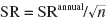 . As we increase the measurement frequency n, we decrease the measured SR.
How frequently you observe profits and losses (P&L), and the corresponding SR, affects how risk is felt. If you observe P&L more frequently—for instance, if you are a hedge fund manager with a live P&L screen—then you have a lower SR between each time you look at the P&L, and the risk is more painful. One way to see why a strategy feels riskier at a frequent time scale is to calculate the probability of observing a loss over a given period. To do so, assume for simplicity that returns are normally distributed (even though that is clearly not the case in the real world). Then we can compute the probability of a loss as follows, where N is a normally distributed random variable with mean zero and a standard deviation of one:
![]()
We see that the probability of losing money simply depends on the SR. The loss probabilities are reported in table 2.1 for the case of a strategy with an annualized SR of 1. We see that even for such a good strategy, the probability of a loss during a 1-minute interval is close to 50%. Hence, even when you have a great year, you probably see losses about every other minute if you are observing the P&L at that frequency. No wonder it can feel so painful.
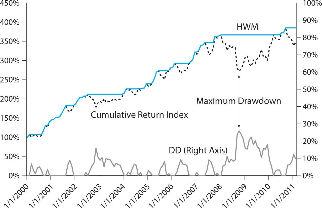
2.5. HIGH WATER MARK
A hedge fund’s high water mark (HWM) is the highest price Pt (or highest cumulative return) it has achieved in the past:
![]()
Often hedge funds only charge performance fees when their returns are above their HWM. Hence, if they have experienced losses, they must first make these back and only charge performance fees on the profits above their HWM.
2.6. DRAWDOWN
An important risk measure for a hedge fund strategy is its drawdown (DD). The drawdown is the cumulative loss since losses started. The percentage drawdown since the peak (i.e., the HWM) is given by
![]()
where Pt is the cumulative return at time t (or share price).3 In other words, the drawdown is the amount that has been lost since the peak (i.e., the HWM). If the hedge fund is currently at its peak, then the drawdown is zero, and otherwise it is a positive number. The drawdown can also be measured relative to other points in time, for example, the beginning of the year. Experiencing large drawdowns is costly and risky. In addition to the direct losses, large drawdowns often lead to redemptions from investors and concerns from counterparties, for example, prime brokers increasing margin requirements or completely pulling the financing of the hedge fund’s positions. When evaluating a strategy, people sometimes consider its maximum drawdown (MDD) over some past time period:
![]()
Figure 2.1 shows an example of a hedge fund strategy and its HWM, drawdown, and MDD.
2.7. ADJUSTING PERFORMANCE MEASURES FOR ILLIQUIDITY AND STALE PRICES
Some hedge funds may not be as hedged as they first appear. To see why, let us consider the following example. Suppose that Late Capital Management (LCM) invests 100% in the stock market but always marks to market one month late. For instance, if the stock market goes up by 3% in January, LCM will report a 3% return in February. In that case, what is LCM’s stock market beta? Well, βLCM will appear to be near zero, since it depends on the covariance with the market and the returns are misaligned in time:
![]()
In other words, since LCM’s return is last month’s market return, and market returns are (close to) independent over time, LCM will appear to have a zero beta in a standard regression:
![]()
The estimated values of α will be the average stock market return, which is positive (over the long term). Hence, LCM appears to be creating alpha from the perspective of the standard estimate, but does marking to market late really create value to investors? Is investing in LCM a good long-term hedge against the market? Clearly not. If you lose on your market investment, you will also lose on your LCM investment next month.
While this example is obviously unrealistic, the general lesson it teaches is more realistic than you may think. Many hedge funds invest in illiquid securities that often do not trade for days, and therefore month-end prices can be “stale.” This problem can be especially severe for securities traded in over-the-counter (OTC) markets with no public price transparency, but it is also an issue for illiquid exchange-traded securities. Hence, the hedge fund returns may be based on stale price marks that do not reflect all the volatility in the market. This delay means that the co-movement with the market (beta) is mismeasured, leading to an inflated measure of alpha. We can adjust for this by regressing not just on the market return during the same period, but also during lagged time periods4:
![]()
The alpha in this multivariate regression now accounts for stale market exposure and captures the hedge fund’s value added beyond its exposure to both current and past market moves. We can then estimate the “true” all-in beta as
![]()
In the example of LCM, this method will produce βall-in = 1 and αadjusted = 0, thus reflecting the true (lack of) value added by this hypothetical hedge fund. This adjustment also makes a significant difference in evaluating many real-world hedge funds and hedge fund indices. We can also adjust other performance measures for the stale-price problem. For instance, to compute the adjusted information ratio, we can use the Sharpe ratio of the all-in hedged returns,  :
:

2.8. PERFORMANCE ATTRIBUTION
Hedge funds frequently review what factors are driving their returns, a process called performance attribution. That is, they look back over the previous quarter, say, and review which trades were the main positive return contributors and which ones detracted. This is useful both for the hedge fund’s communication with its clients and for internal planning and evaluations. From the hedge fund investors’ perspective, performance attribution is useful because it provides insight into the investment process, the drivers of returns, and the risk factors to which they are exposed. Internally, in a hedge fund, performance attribution can be used to determine which investment strategies appear to be working and which traders tend to make successful investments.
2.9. BACKTESTS VS. TRACK RECORDS
It is important to distinguish between performance measures that are gross versus net of transaction costs and gross versus net of fees. Whether to consider performance before or after transaction costs and fees depends on what the measure is used for. Investors clearly care about a hedge fund’s performance after transaction costs and after fees—they enjoy only these net returns. A hedge fund’s track record is its realized performance after all fees and costs over its life. Some hedge funds have different fee schedules (e.g., one option with a high management fee and no performance fee and another option with a low management fee and a high performance fee), in which case they must report the track record using the most conservative fee schedule.
Hedge funds also consider backtests of their strategies, that is, historical simulations of their performance under assumptions about how they would have behaved in the past. While investors are ultimately interested in net returns, a hedge fund might internally investigate a trading idea by first looking at the gross return in a backtest. Indeed, the hedge fund may first try to determine whether a strategy has any merit and, for this, examine whether the gross returns appear to be reliably positive. If the strategy appears to make money, the hedge fund will next consider whether the strategy survives transaction costs and, ultimately, whether it will add value for investors. While the fund’s realized returns are naturally net of transaction costs, how to adjust a backtest for transaction costs is more involved. We next consider in more detail how to construct a backtest, how to account for trading costs, and how to consider a trade’s leverage and financing issues.
___________________
1 This second definition of the IR is equivalent to the first definition if we set β equal to one in the benchmark regression.
2 For instance, mutual funds are required to report geometric averages in the United States.
3 This drawdown formula is based on a cumulative return index Pt computed using compounding, that is, Pt = Pt−1 × (1 + Rt). If the cumulative return index is computed by simply adding up returns (or log returns), that is, Pt = Pt–1 + Rt, then the drawdown is also defined in an additive way, DDt = HWMt − Pt. Also, some investors think of drawdowns as negative numbers, so they put a minus sign in front of my definition.
4 This issue was pointed out by Asness, Krail, and Liew (2001), who suggested the lagged beta methodology due to Scholes and Williams (1977) and Dimson (1979).