Portfolio Construction and Risk Management
A hedge fund’s job is to deliver the best possible risk-adjusted returns. To do so, the hedge fund must first find trades that can be expected to make money, as discussed earlier. Once several trading strategies have been identified, the investor must combine them into an overall portfolio. Portfolio construction means (i) estimating the risk that each trade involves and (ii) choosing how to size each of the positions and how to vary these position sizes over time to achieve an optimal trade-off between risk and expected return.
Active investors must put special emphasis on risk management. Risk management should be an integral part of portfolio construction and, in addition, a hedge fund should have a separate risk management team with an independent set of controls. The risk of a hedge fund portfolio changes over time for a number of reasons. First, investment opportunities vary, and people often want to invest more when the opportunities are better. Second, market risk varies over time so that the same positions can be more or less risky, depending on the circumstances. Third, the hedge fund’s different bets may be more or less aligned with one another at different times. Fourth, the use of leverage means that a hedge fund cannot always “ride out” a drawdown; it must be ready to react before creditors pull their financing or investors pull their capital.
Portfolio construction should rely on continuously updated measures of risk and should ensure that the risk taken is at an appropriate level given the opportunities. The risk management overlay must simultaneously ensure that the risk never exceeds certain limits, manage the downside tail risk, and limit the risk of large drawdowns.
4.1. PORTFOLIO CONSTRUCTION
Active investors differ a great deal in their portfolio construction, with some relying on rules and intuition while others use computer algorithms to perform a formal portfolio optimization. However, there are some general principles that most successful hedge funds adhere to:
• The first principle of portfolio construction is diversification. Indeed, the saying goes that the only free lunch in finance is diversification.
• The second principle is to have position limits, which restrict the notional exposure to each security and/or its risk contribution. For example, when I have taught my class on hedge fund strategies, I have often presented MBA students with a great trade, for instance, a pure arbitrage such as one of the negative stub trades (discussed further in chapter 16, event-driven investments). Once the students have figured out the trade, I ask them to size the position, and most students invest at least 40% of their capital in the trade. The following week, we see how they would have fared. Almost every student’s position blows up (except one or two students who would not do the trade at all). Indeed, simulating their margin equity shows that they could not meet their margin calls and were forced to liquidate most of their position, thus ending up with a loss, or completely broke, even when the trade finally converged. One simple and effective way to reduce the risk of being blown up by a single position—and ensure greater diversification—is to have position limits. For instance, James Chanos makes sure that all his positions are less than 5% of his net asset value (NAV), trimming positions back as they approach this limit.
• A third principle of portfolio construction is that you should make larger bets on higher conviction trades. You need to think about what trades are really promising and make sure that this is where you are taking the most risk.
• A fourth principle is that you should think of the size of a bet in terms of its risk. The magnitude of a position’s risk depends both on the notional size of the position and the risk of the underlying security.
• A fifth principle is that correlations matter. For a long position, a high correlation with other longs is bad, whereas a high correlation with short positions is good. For example, Lee Ainslie prefers to have both long and short positions within each industry, thus having risk reduction through being long and short in similar securities. Furthermore, his longs are diversified across industries, thus having risk reduction through long positions with low correlations.
• The final principle is to continue to resize positions according to risk and conviction. As important as this is, many people find this unintuitive. As one student said as his simulated profit and loss (P&L) turned south: “I am in this trade with both feet, and there is no turning around now.” Two simulated days later, he was out of business. Successful hedge funds don’t marry their positions and don’t let their bets grow large inadvertently. For instance, Lee Ainslie continues to analyze each trade’s risk–reward trade-off and then decides to add or reduce its position. “Hold” is not an option. A related trader saying goes that
A trader must have no memory and forget nothing.
An investor should have “no memory” in the sense that she should do what is optimal on a going-forward basis, regardless of how she got into the current position. An investor should “forget nothing” in the sense that all his or her experiences and data should help make the best possible forecasts of risk and expected return.
Quants such as Cliff Asness use formal portfolio optimization to achieve these goals. Indeed, when trading thousands of securities around the world, you need computing power to effectively implement these portfolio construction principles. The simplest way to do this is a mean-variance approach: The goal is to choose a portfolio x = (x1, …, xS), where xs measures the capital (i.e., the amount of money) invested in each security s. If you start with a wealth of W and choose the portfolio x, then your wealth next time period is
![]()
where R1, …, RS are the returns of the different risky investments, and the last term captures the money invested in the risk-free money market with return Rf (or the money borrowed for leverage if the sum of the risky investments is larger than the initial wealth W). The expression for the future wealth can be rewritten in terms of excess returns Re,s = Rs – Rf:
![]()
In other words, the future wealth is the current wealth W increased at the risk-free rate plus all the excess returns you make by investing in risky assets. The goal is to maximize the expected future wealth, subject to a penalty for risk as measured by variance. The portfolio optimization problem can be written using vector notation (ignoring the first term that does not depend on x) as
![]()
where γ is a risk aversion coefficient. If we write the vector of expected security excess returns as E(Re) and the variance–covariance matrix as , the portfolio problem can be rewritten as
![]()
To solve this problem, we consider the first-order condition by differentiating with respect to x and setting this equal to zero:
![]()
which gives the optimal portfolio
![]()
This optimal portfolio is characterized by taking large positions for securities with large expected returns, low variance, and low correlation to other positions.
While optimal in theory, this portfolio is often problematic in practice for several reasons (Black and Litterman 1992). First, the theoretically optimal portfolio may behave poorly in practice because the risk and expected returns are estimated with errors and often using different techniques. Using noisy risk and return estimates that come from different sources often leads the optimizer to suggest extremely large long and short positions with poor out-of-sample performance. Hence, quants try to make the portfolio optimization more “robust” in the sense that it is less sensitive to noise. To achieve a more robust portfolio, they shrink estimates of risk and expected returns, use portfolio constraints, and apply robust optimization techniques. A second problem with the basic mean-variance optimal portfolio is that real-world portfolios are often subject to a number of limits on position sizes and trade sizes, and, while these constraints can be added to the problem, they often distort the solution unless handled carefully. A third issue of a basic one-period optimized portfolio is that it does not take into account that investors trade repeatedly over time and incur transaction costs in the process, but these issues can be handled in a more sophisticated dynamic model (Gârleanu and Pedersen 2013, 2014).
Despite these challenges, portfolio optimization can be a very useful tool, but a full treatment of this topic is beyond the scope of this text. When done carefully, portfolio optimization provides a tool to reap the full benefits of diversification, to efficiently exploit high-conviction trades without excessive concentration, to systematically adjust positions based on the time-varying risk and expected return, and to minimize subjectivity in the portfolio choice.
In summary, good portfolio construction techniques can help achieve a favorable risk-return profile for a set of trading ideas. A systematic approach helps reduce a trader’s own behavioral biases, that is, his tendencies to make certain mistakes. For instance, people like to hang on to their losing positions even if the reason they liked the securities no longer applies, and they like to sell winners to lock in gains even if the trade has gotten even better.
4.2. RISK MANAGEMENT
Measuring Risk
Risk can be, and should be, measured in several different ways. One straightforward and common risk measure is volatility (that is, the standard deviation of returns). Some people think that volatility only applies to normal distributions, but this is not true. What is true is that volatility does not capture well the risk of crashes for non-normal distributions. Indeed, while for normal distributions two–standard-deviation returns are uncommon and five–standard-deviation events almost never happen, this is not true for real-world hedge fund returns since they are not normally distributed. For hedge fund strategies, two–standard-deviation events are common and five–standard-deviation events certainly do happen. If this fact is kept in mind, volatility can still be a useful risk measure as long as the return distribution is relatively symmetric and without too extreme a crash risk. However, volatility is not an appropriate measure of risk for strategies with an extreme crash risk. For instance, volatility does not capture well the risk of selling out-the-money options, a strategy with small positive returns on most days but infrequent large crashes. To compute the volatility of a large portfolio, hedge funds need to account for correlations across assets, which can be accomplished by simulating the overall portfolio or by using a statistical model such as a factor model.
Another measure of risk is value-at-risk (VaR), which attempts to capture tail risk (non-normality). The VaR measures the maximum loss with a certain confidence, as seen in figure 4.1 below. For example, the VaR is the most that you can lose with a 95% or 99% confidence.
For instance, a hedge fund has a one-day 95% VaR of $10 million if
![]()
A simple way to estimate VaR is to line up past returns, sort them by magnitude, and find a return that has 5% worse days and 95% better days. This is the 95% VaR, since, if history repeats itself, you will lose less than this number with 95% certainty. You can estimate the VaR by looking at your past returns, but if your positions have changed a lot, this can be rather misleading. In that case, it may be more accurate to look at your current positions and simulate returns on these positions over, say, the past three years.
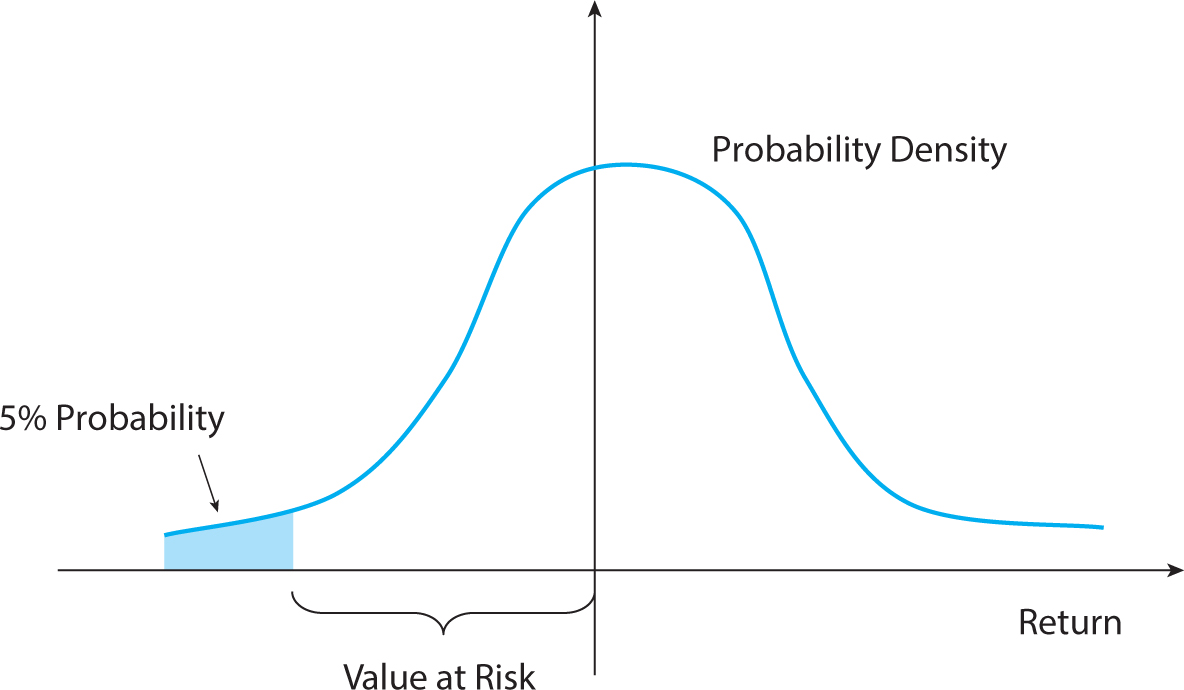
Figure 4.1. Value-at-risk.
The x-axis has the possible outcomes for the return, and the y-axis has the corresponding probability density.
One issue with the VaR is that it does not depend on how much you lose if you do lose more than the VaR. The magnitude of these extreme tail losses is, in principle, captured by the risk measure called the expected shortfall (ES). The expected shortfall is the expected loss, given that you are losing more than the VaR:
![]()
Another measure of risk is the stress loss. This measure is computed by performing various stress tests, that is, simulated portfolio returns during various scenarios, and then considering the worst-case loss in these scenarios. Such stress scenarios can include significant past events, such as the 1998 price shocks around the Long-Term Capital Management (LTCM) bailout, September 11, and the failure of Lehman Brothers, as well as imagined future events, such as the failure of a sovereign state (e.g., Greece), a large interest rate move, a large shock to equity prices, a spike in volatility, or a sharp increase in margin requirements.
While estimates of volatility and, to some extent, VaR measure the risk during relatively “normal” markets over a fixed time horizon, stress tests tell you about risk during extreme events. Indeed, volatility and VaR are statistical measures of day-to-day risk that rely on having enough data to estimate them. Stress tests explore cases where you do not have enough data to estimate the risk accurately, as well as events that can play out over several days. An important risk that may not be captured by volatility estimates is the risk of liquidity spirals, as discussed before. The point of a stress test is to make sure that positions are not so large that the hedge fund is likely to blow up in a stress event and to plan for foreseeable events, even if you cannot predict losses or give probability estimates. Of course, what actually happens during a crisis never corresponds exactly to any stress tests, but one hopes that preparing for foreseeable events will provide the discipline to survive what actually happens.
Risk Management: Prospective Risk Control
Whatever the measure of risk, risk needs to be managed. Risk management should be both prospective (i.e., controlling risk before a bad event occurs) and reactive (having a plan for what to do in a crisis). Reactive risk management is usually a form of drawdown control (discussed in detail below) and stop-loss mechanisms.
Even before you react to losses, you can manage risk prospectively. Prospective risk management comes in several forms, including diversification, risk limits, liquidity management, and tail hedging via options and other instruments.
To control risk, a hedge fund often has risk limits, meaning prespecified restrictions on how large a risk the hedge fund will ever take. The risk limit can be at the overall fund level and/or at the more granular level of each asset class or strategy. Hedge funds often also have position limits that restrict the notional exposure (regardless of how low the risk is estimated to be).
Furthermore, some hedge funds have a strategic risk target, meaning an average level of risk that the fund intends to take over the long term. For instance, the strategic risk target could be measured as the fund volatility, and it would often range from bondlike volatility to equitylike volatility, say, somewhere between 5% and 25% annualized volatility. The hedge fund’s desired risk at a given time is sometimes called the tactical risk target, and the tactical risk varies around the strategic risk target, depending on the investment opportunities, market conditions, and recent performance. In particular, significant losses often drive a hedge fund to reduce positions and cut risk, that is, reactive risk management, as discussed next.
4.3. DRAWDOWN CONTROL
While prospective risk control seeks to manage the portfolio risk before losses occur, drawdown control is a reactive mechanism that seeks to limit losses as they evolve. Drawdown control is important for hedge funds using leverage because they cannot simply decide to always “ride out” a crisis. A hedge fund may therefore want to minimize the risk that its drawdown will become worse than some prespecified maximum acceptable drawdown (MADD), say, 25%.1 If the current drawdown is given by DDt, then one sensible drawdown control policy is
![]()
The right-hand-side of this inequality is the distance between the maximum acceptable drawdown and the current drawdown, that is, the largest acceptable loss given the amount already lost. The left-hand-side is the value-at-risk, that is, the most that can be lost given the current positions and current market risk, at a certain confidence level. Hence, the drawdown policy states that the risk must be small enough that losses do not push drawdowns beyond the MADD, with a certain confidence.
If this inequality is violated, the hedge fund should reduce risk, that is, unwind positions such that the VaR comes down to a level that satisfies the inequality. Once the strategies have recovered and the drawdown is reduced, the risk can be increased again.
To make this drawdown system operational, one must choose a MADD and also the type of VaR measure to use on the left-hand side (i.e., the time period and the confidence level). This choice depends on the risk and liquidity of the hedge fund. A lower risk fund may have investors and counterparties with less tolerance for drawdowns and should therefore have tighter limits. A riskier fund, on the other hand, should have looser limits so that the drawdown system does not kick in too often in order to limit transactions costs—if you take a large amount of risk, you must live with larger drawdowns.
Drawdown control is helpful because it creates a clear plan for how to handle adversity: how much to reduce risk when you are losing money and when to do it. Without a clear plan for drawdown control, traders may have difficulty controlling their emotions during tough periods. Indeed, reducing risk after losing on a position is painful. The trader feels that a loss is being locked in if she unwinds and often prefers to try to ride out the situation—until growing losses turn into a disaster. Risk management is far from always a losing proposition, however. It can save an investor a tremendous amount, as the saying goes:
Your first loss is your least loss.
As discussed in section 5.10, prices tend to drop and rebound during a liquidity spiral where some traders are forced to unwind. Traders often end up holding onto their positions as prices fall, but eventually they have to cave and sell near the bottom as their funding dries up or panic ensues. Why are most of them selling near the bottom? Because this defines the bottom. When the selling is over, prices start rebounding. This logic may be what is behind the following saying:
As a trader, never panic, but if you are going to panic, panic first.
And it almost surely underlies the following poker-related maxim:
The strongest weak hand suffers the largest loss.
Using a poker analogy, one can distinguish between “strong hands” and “weak hands.” Strong hands have what it takes to hold onto their positions, or even add to them at low prices. They have deep pockets and the emotional strength to live through a crisis. In contrast, weak hands must sell their positions if they incur large losses. For instance, leveraged hedge funds are weak in the sense that they can hit their margin constraint and be forced to liquidate, or their prime broker can pull the plug even before that happens. The weak hands that “panic first” and fold almost immediately suffer lower losses than the “strongest weak hands,” which are forced to sell at the bottom. Of course, traders never know whether they will end up being able to ride out the crisis or be forced to liquidate, but a sound drawdown policy planned in advance without emotional stress is a good idea.
A prespecified plan for drawdown control not only helps reduce risk in a timely manner, but it can also help investors re-enter the market in time to re-coup (some of) the losses. A trader who was just forced to cut risk may be “burned” and afraid to scale the positions back up, but a systematic drawdown control system signals it is time to re-enter the market when positions have recovered sufficiently and risk has declined.
___________________
1 This section draws from Grossman and Zhou (1993).