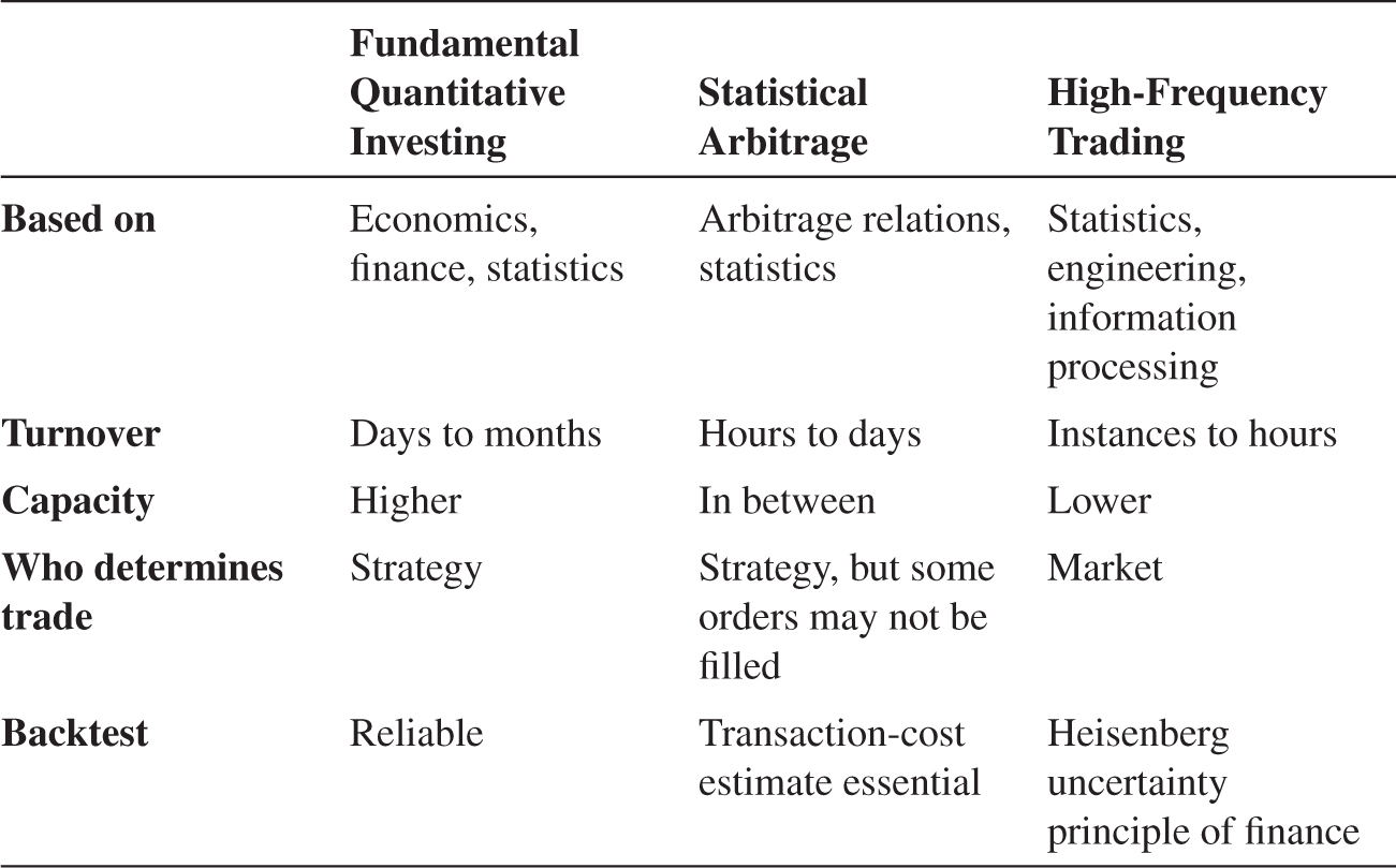
TABLE 9.1. THREE TYPES OF QUANTITATIVE INVESTING
Quantitative Equity Investing
I think that good quant investment managers … can really be thought of as financial economists who have codified their beliefs into a repeatable process. They are distinguished by diversification, sticking to their process with discipline, and the ability to engineer portfolio characteristics.
—Cliff Asness (2007)
Quantitative equity investing—quant equity, for short—means model-driven equity investing, performed, for instance, by equity market neutral hedge funds. Quants codify their trading rules in computer systems and execute orders with algorithmic trading overseen by humans.
There are several advantages and disadvantages of quantitative investing relative to discretionary trading. The disadvantages are that the trading rule cannot be as tailored to each specific situation and it cannot be based on “soft” information such as phone calls and human judgment. These disadvantages may be diminishing as computing power and sophistication increase. For instance, quant models may analyze transcripts of a firm’s conference calls with equity analysts using textual analysis, looking at whether certain words are being frequently used or doing more complex analysis.
The advantages of quantitative investing include, first, that it can be applied to a broad set of stocks, yielding significant diversification. When a quant has constructed an advanced investment model, this model can be simultaneously applied to thousands of stocks around the world. Second, the quant’s modeling rigor may largely overcome the behavioral biases that often influence human judgment, perhaps those very biases that create the trading opportunities in the first place. Third, the quant’s trading principles can be backtested using historical data. Quants view data and scientific methods as central to investing:
We are misguided when we exalt ourselves by insisting that the psychology of the marketplace and of man are unknowable. The sciences of man are now emerging from the Dark Ages. Economics and psychology stand today at Koestler’s watershed just as astronomy did in the time of Tycho Brahe. Our superstition, blind belief, and ignorance are being swept away forever by the scientific accumulation and analysis of data. There will be predictability in the affairs of men.
—Thorp and Kassouf (1967)
Quantitative equity can be subdivided into three types of trades: fundamental quant, statistical arbitrage (stat arb), and high-frequency trading (HFT), as seen in table 9.1. These three types of quant investing differ along several dimensions, including their intellectual foundation, their turnover, their capacity, how trades are determined, and the extent to which they can be backtested.
Fundamental quantitative investing seeks to apply fundamental analysis—just like discretionary traders—but does so in a systematic way. Fundamental quant is therefore based on economic and finance theory along with statistical data analysis. Given that prices and fundamentals change only gradually, fundamental quant typically has a turnover of days to months and has a high capacity (meaning that a lot of money can be invested in the strategy) also due to significant diversification.
Stat arb seeks to exploit relative mispricings between closely related stocks. Hence, it is based on an understanding of arbitrage relations and statistics, and its turnover is typically faster than that of fundamental quants. Due to the faster trading (and perhaps fewer stocks with arbitrage spreads), stat arb has a smaller capacity.
TABLE 9.1. THREE TYPES OF QUANTITATIVE INVESTING
Finally, HFT is based on statistics, information processing, and engineering, as an HFT’s success depends partly on the speed with which they can trade. HFTs focus on having superfast computers and computer programs and co-locating their computer at the exchanges, literally trying to get their computer as close as possible to the exchange server, using fast cables, etc. HFTs have the fastest turnover of their trades and naturally have the lowest capacity.
The three types of quants also differ in the way trades are determined: Fundamental quants typically determine their trades ex ante, stat arb traders determine their trades gradually, and HFTs let the market determine their trades. More specifically, a fundamental quant model identifies high-expected-return stocks and then buys them, almost always getting their orders filled; a stat arb model seeks to buy a mispriced stock but may terminate the trading scheme before completion if the prices have moved adversely; finally, an HFT model may submit limit orders to both buy and sell to several exchanges, letting the market determine which ones are being hit. This trading structure means that fundamental quant investing can be simulated via a backtest with some reliability; stat arb backtests rely heavily on assumptions on execution times, transaction costs, and fill rates; while HFT strategies are often difficult to simulate reliably so HFTs must also rely on experiments.
HFT is subject to what one could call the Heisenberg uncertainty principle of finance. In physics (quantum mechanics), the Heisenberg uncertainty principle states that there is a limit to the precision with which one can know a particle’s position and momentum because the act of observing disturbs the particle. Analogously, one cannot simulate with precision the timing and price of execution of a limit order because the act of submitting the order changes the market dynamics.
9.1. FUNDAMENTAL QUANTITATIVE INVESTING
Fundamental quants trade on factors such as value, momentum, quality, size, and low risk. They use information similar to that used by discretionary traders, but they effectively try to “teach” a computer what a great equity analyst does and then apply this methodology across thousands of stocks around the world in a systematic manner.
Fundamental quant investing can be applied both in a long-only and long–short context. In fact, given that quant models often have views on all stocks in the investment universe, these views can be naturally applied in several contexts such as long–short market-neutral hedge fund strategies, 130/30 long-biased strategies, and long-only benchmark-driven strategies. The underlying building block is the same, namely the quantitative estimates of which stocks have high expected returns, which ones have low expected returns, and a risk model. The long–short hedge fund portfolios are often combinations of several “factors,” meaning that long–short portfolios that are regularly rebalanced to bet on a specific phenomenon. At the same time, these factors are useful representations of which stocks have high vs. low expected returns and therefore are also useful for the other types of quant equity investing. We start by considering the value factor, which captures the return to quant-style value investing.
Value Investing, Quant Style
Quants perform value investing by systematically computing a measure related to a stock’s fundamental value (the present value of future free cash flows) and comparing it to the stock’s current market value. Quants then buy value stocks—those with high ratios of fundamental value to market value—and sell those with the opposite characteristics.
One might think that such a strategy only works if it is based on an extremely good measure of the fundamental value, one that contains more information than the market price. This intuition is not correct in general, though, which might be surprising. The reason is that prices depend not only on expected future cash flows but also on how these are discounted, that is, prices reflect expected returns. Said simply, value investing works because the price equals the expected cash flows divided by the expected return—so, flipping this equation around, the expected return is cash flows divided by price. Hence, value investing may work for any variable that can reasonably be used to normalize the price.
As a case in point, value investing has worked historically even for very simple measures of value such as a stock’s book to market (BM), that is, the ratio of the book value of equity to the market value of equity.1 Of course, the book value is a somewhat simplistic measure of the fundamental value with all the issues related to accounting variables (including that it is backward looking, not forward looking), but it nevertheless serves as a useful scaling variable for market values.
Based on variation in stock’s expected returns, value stocks are likely to be those with high expected returns, which could either be driven by rational compensation for risk, by institutional frictions, or by behavioral reasons. Some economists (e.g., Keynes 1936, Shiller 1981, and Lakonishok, Shleifer, and Vishny 1994) have argued that stocks vary excessively, which creates opportunities for value investors:
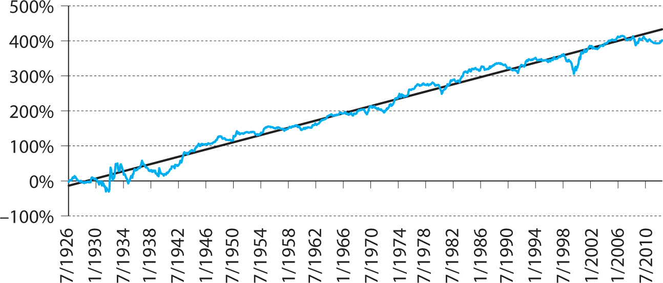
Figure 9.1. Cumulative performance of the value factor HML, 1926–2012.
The figure shows the cumulative sum (i.e., without compounding) of the long–short value factor HML constructed based on stocks’ book-to-market ratios.
day-to-day fluctuations in profits of existing investments, which are obviously of an ephemeral and nonsignificant character, tend to have an altogether excessive, and even absurd, influence on the market
—John Maynard Keynes (1936)
Value investing has worked on average historically, as seen in figure 9.1, which plots the cumulative returns to the high-minus-low (HML) factor of Fama and French (1993). HML goes long on the 30% stocks with the highest book-to-market scores—i.e., the cheapest stocks by this measure—and shorts the 30% most expensive stocks.2 By being balanced long and short, the return of HML captures the outperformance of cheap stocks relative to expensive stocks, thus eliminating any direct effect of overall market movements. Over this time period, HML has delivered an average excess return of 4.6% per year with an annual volatility of 12.3%, corresponding to a Sharpe ratio of 0.4.
Value investing also works based on other value measures such as earnings-to-price, dividends-to-price, and cash flows-to-price, and it can be refined further by considering the quality of a stock as discussed below.
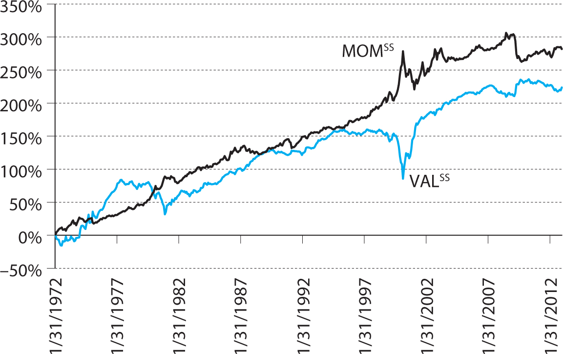
Value strategies have also worked across regions and asset classes. Value strategies have worked in global stock markets, including in the United Kingdom, continental Europe, and Japan, and they have worked in other asset classes, such as commodities and currencies (Cutler, Poterba, and Summers 1991 and Asness, Moskowitz, and Pedersen 2013). Interestingly, value strategies in different regions and asset classes tend to be positively correlated, suggesting a common global systematic risk factor, which could be consistent with a risk-based explanation for value investing. As seen in figure 9.2, the returns to value investing are negatively correlated with another important quant equity strategy, namely momentum investing, which we discuss next.
Figure 9.2. Performance of global value and momentum stock-selection strategies, 1972–2012.
The graphs show the cumulative sums of monthly returns of the value and momentum strategies across the United States, United Kingdom, continental Europe, and Japan (Asness, Moskowitz, and Pedersen 2013).
Stock Momentum: Quant Catalysts
Momentum investing means buying recent winners and short-selling recent losers. Specifically, the strategy plotted in figure 9.2 considers each stock’s performance over the most recent year (leaving out the most recent month, as discussed further below) and goes long on the stocks that had the highest returns while shorting those that had the lowest returns. As seen in the figure, momentum has worked quite well, historically producing an even higher return than value investing, at least before transaction costs.3
The strong performance of momentum investing means that stocks that have been outperforming over the past 12 months tend to continue to outperform over the following month. It is hard to justify momentum with a rational risk premium because the high turnover of momentum would imply that a stock’s risk characteristics should quickly and frequently change. Perhaps a more appealing story is that stocks exhibit an initial underreaction to news and then perhaps a delayed overreaction. It may be surprising that both underreaction and overreaction can drive momentum profits, but here is why: First, good news today leads to a price increase today, but, if price initially underreacts, then the price must continue to go up in the future—i.e., producing momentum. Second, if prices have been going up for a while and investors start to jump on the bandwagon leading to a delayed overreaction, then this further adds to the momentum.
Another way to conceptualize the momentum is to think of it as a quant measure of equity catalysts. Recall, as discussed in chapter 7, that discretionary equity investors are often looking for stocks that have value plus a catalyst, meaning cheap stocks where the market is about to recognize their potential. Such a catalyst can make the value bet pay off quickly as the stock price rises, rather than the equity analyst having to wait for his profit until the company actually delivers on its potential with all the risks that comes with waiting. High-momentum stocks are stocks that have been outperforming and, therefore, may be increasingly popular among investors. Combining value and momentum investing is a powerful cocktail since these strategies are negatively correlated and, therefore, the combination delivers higher risk-adjusted returns than either one does alone. A stock that has favorable value and momentum characteristics is a cheap stock on the rise, which has a better chance of continuing its trend than an average momentum stock (because it is still cheap) and a better a chance of delivering on its value (because potential investors are starting to recognize it).
Quality Investing: Systematizing Graham and Dodd
Just as momentum investing is a natural complement to value investing, so is quality investing (but for a different reason). Quality investing is the strategy of buying high-quality stocks. High-quality stocks can be defined as stocks that are profitable, growing, stable, and well managed, as discussed in section 7.2. Different investors might have different views of each of these quality components, but considering a variety of such quality measures, Asness, Frazzini, and Pedersen (2013) find that quality factors have delivered positive excess returns on average for both U.S. and global stocks and for both small and large stocks.
Quality investing buys “good” stocks that deserve a higher-than-normal price (or price-to-book ratio) and short-sells “bad” stocks that deserve to be cheap. In contrast, simple value factors short-sell the expensive stocks (whether or not the expensiveness is justified by the stocks’ quality characteristics) and buys the cheap ones (whether or not they deserve to be cheap). Hence, quality investing complements simple value investing and, indeed, quant value and quality factors tend to be negatively correlated.
Combining value and quality factors gives rise to a strategy that can be called “quality at a reasonable price,” which has higher risk-adjusted returns than each component alone. Combining quality, value, and momentum yields an even stronger strategy that buys upward-trending stocks that are cheap relative to their quality and shorts falling stocks that are expensive.
Betting against Beta and Low-Risk Investing
The classic capital asset pricing model (CAPM) says that a security’s expected excess return should be proportional to its beta, 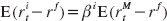 . Hence, if stock A has a beta of 0.7 and stock B has twice the beta of 1.4, then stock B should have twice the excess return on average. However, the CAPM does not hold empirically as the average returns of low-beta stocks is almost as high as the average return of high-beta stocks. In the lingo of the CAPM, the security market line (SML) is too flat empirically, as seen in figure 9.3.
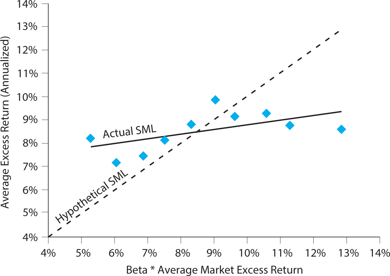
Figure 9.3. The security market line is too flat relative to the CAPM.
The figure plots ten dots corresponding to ten U.S. stock portfolios sorted by their ex ante beta, 1926 to 2010. The horizontal axis shows the CAPM-predicted return for each portfolio, i.e., its ex post realized beta multiplied by the market risk premium,  . The vertical axis plots each portfolio’s actual average excess returns, corresponding to
  . The 45-degree line is the hypothetical SML implied by the CAPM.
What should you do if the data do not fit the theory? Reject the theory or exploit that the financial market doesn’t behave as it “should.” But how could you exploit the flat security market line? Well, the safe stocks are the ones that have high returns compared to what the CAPM says they should. Said differently, the safe stocks have positive alpha and the risky stocks have negative alpha.
So, you should probably buy the safe stocks and short-sell the risky ones. Does that make money? No, not if you buy $1 of safe stocks and short $1 of risky ones. As seen in figure 9.3, the five portfolios with the riskiest stocks have slightly higher average returns than the five safest portfolios. However, buying safe stocks and shorting risky ones also would not be a market-neutral portfolio because, by construction, the long side is much safer than the short side.
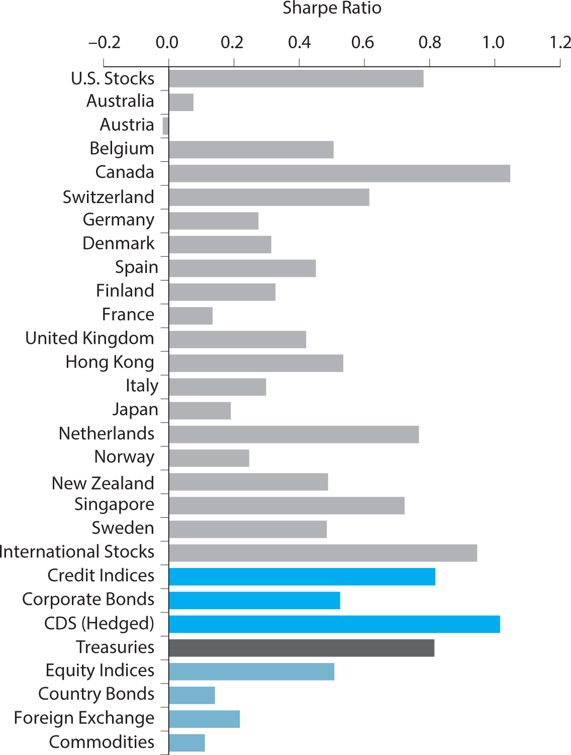
To have a market-neutral portfolio, you need to buy about $1.4 worth of safe (i.e., low-beta) stocks and short-sell $0.7 worth of risky (high-beta) stocks. This portfolio does make money because it exploits the fact that, while safe and risky stocks have similar average returns, the safe stocks have significantly higher Sharpe ratios. This portfolio exploits the differences in Sharpe ratios by leveraging the safe shorts and deleveraging the risky ones so that both the long and short sides of the portfolio have a beta of 1. The portfolio is called a “betting against beta” (BAB) factor. The BAB factor for U.S. stocks has realized a Sharpe ratio of 0.78, as seen in figure 9.4. As also seen in the figure, the BAB factor has had positive performance in most global stock markets as well as in the credit markets, bond markets, and futures markets.
One reason that low-risk investing has worked is that many investors face leverage constraints or are simply afraid of the risks that comes with leverage. Therefore, investors looking to pick up a higher return might buy risky securities rather than applying leverage to a portfolio of safe securities. This behavior pushes up the prices of risky stocks—and high prices mean low returns. This behavior simultaneously lowers the demand for safe stocks, lowering their prices and increasing their expected returns. Hence, a modified CAPM equilibrium arises in which the security market line is flatter due to leverage-constrained investors buying the risky stocks while less constrained investors leverage the safer stocks. This BAB theory can therefore explain why mutual funds and individual investors (who might be leverage constrained or averse) hold stocks with betas above one on average while Warren Buffett and leveraged buyout (LBO) investors apply leverage to safer stocks on average.4
There are also several other forms of low-risk investing. Some long-only investors buy safe stocks without shorting risky stocks. This method should earn an average return just below the overall market return with a significantly lower risk, thus realizing a higher Sharpe ratio. Rather than focusing on low-beta stocks, other investors focus on stocks with low total volatility, low idiosyncratic volatility, low earnings volatility, high-quality stocks, or seek to construct the minimum-variance portfolio.
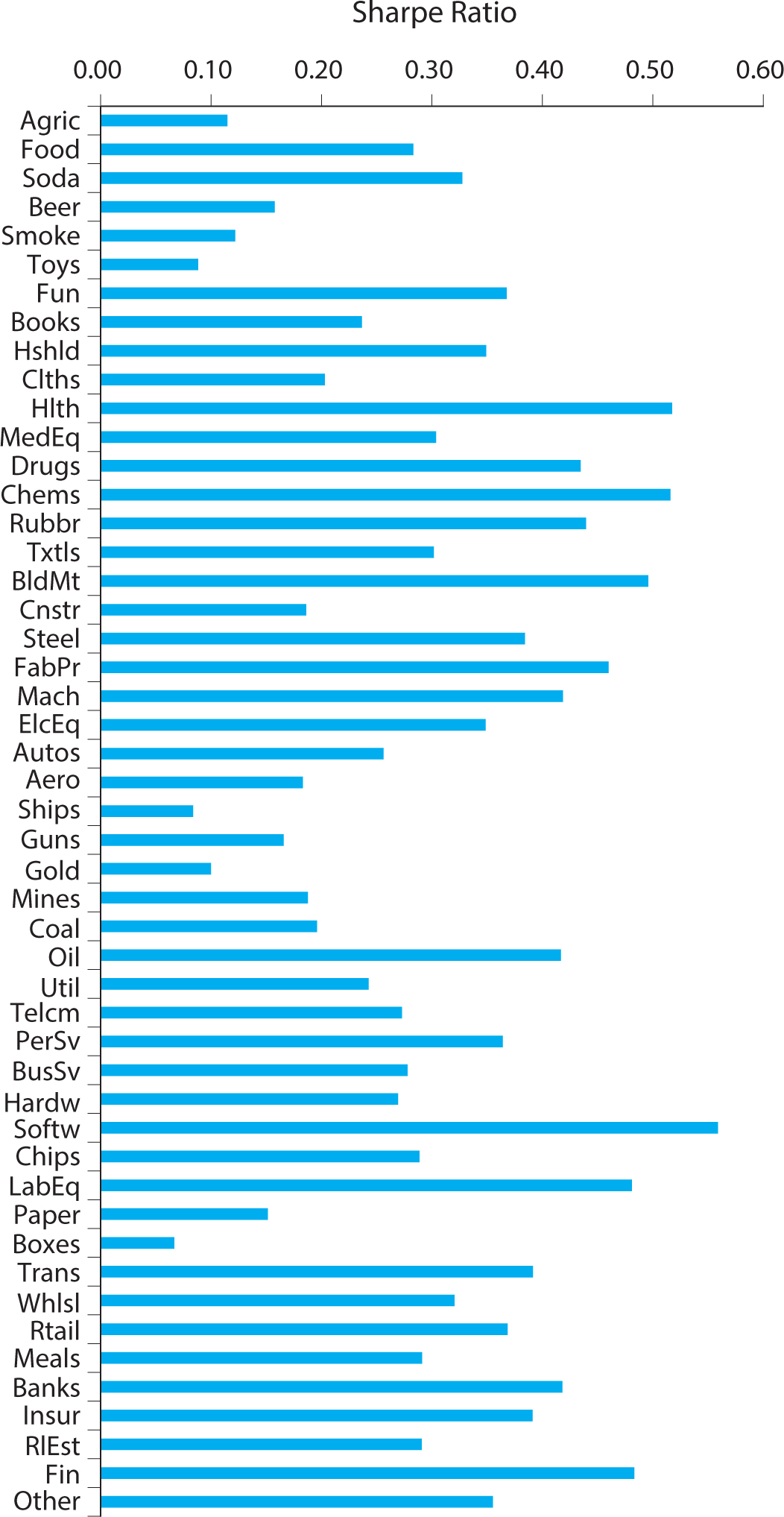
A low-risk portfolio constructed without regard to industries or sectors tends to overweight stocks in non-cyclical industries such as utilities, retail, or tobacco stocks. However, these industry bets are not the main reason that low-risk investing works. In fact, low-risk investing has historically worked both for investing across and within industries. Figure 9.5 shows BAB factors constructed within each industry in the United States. For example, the BAB factor for utility stocks goes long on a leveraged portfolio of the safer utility stocks while shorting the riskier utility stocks. Remarkably, low-risk investing has worked within each industry in the United States.
Figure 9.5. Betting against beta strategies within each U.S. industry, 1926–2012.
Each bar plots the Sharpe ratio of a BAB strategy within an industry.
Source: The data are based on Asness, Frazzini, and Pedersen (2014).
Quants apply their models across hundreds or even thousands of stocks. This diversification eliminates most of the idiosyncratic risk, meaning that firm-specific surprises tend to wash out at the overall portfolio level and any single position is too small to make a significant dent in the performance.
By being equally long and short, an equity market neutral quant portfolio also eliminates the overall stock market risk. Some quants try to achieve market neutrality by making sure that the dollar exposure on the long side equals the dollar value of all the short positions. However, this method only works if the longs and shorts are equally risky. Hence, quants also try to balance to market beta of the long and the short side. Some quants try to be both dollar neutral and beta neutral.
Quants also often eliminate (some) industry risk. For each industry, they may go long on the “good” stocks in the industry while shorting the “bad” ones, thus being neutral to the overall movement in the industry. For instance, figure 9.5 shows the performance of industry-neutral BAB factors, which can be combined into an overall industry-neutral factor. This industry-neutral portfolio construction can create a higher Sharpe ratio for two reasons. First, it eliminates industry risk. Second, it may pick “good” stocks more accurately because the portfolio is constructed by comparing industry peers, which is often a more meaningful comparison. If a factor also works for selecting industries—as momentum does, for instance—then quants may both bet on within-industry momentum and across-industry momentum, controlling the amount of risk arising from each bet.
When a quant has eliminated (most of) the idiosyncratic risk, market risk, and industry risk, then what risk is left? No risk at all? Surely not. The risks that are left are the risks associated with the factors that the quant wants to bet on. If a quant is betting on value, for instance, her portfolio risk is that the value factor performs poorly. A value-based portfolio loses if cheap stocks get cheaper and expensive stocks get more expensive or if the “cheap” stocks turn out not to be cheap relative to their deteriorating fundamentals. Hence, like all leveraged investors, quants face the risk of a liquidity spiral like the one that happened in the 2007 quant event, as we discuss later.
While we have discussed the general tricks of quant investing, there are many differences in the specifics of quant portfolio construction. Some quants seek to control the volatility of their portfolios, whereas others keep a constant notional exposure. Some try to tactically time which factors are more likely to work at any time, and others keep a constant weight on each factor. Quants also differ in how they get from each stock’s signal to its weight in the portfolio. Academic factors traded only on paper often buy the top 10% stocks with the most favorable characteristics while shorting the bottom 10%, rebalancing the paper portfolio each month. This strategy leads to a large turnover and is therefore rarely used in practice. Quants try to estimate the relation between the signal value and the expected return and construct the portfolio and the rebalancing strategy that maximizes performance after transaction costs.
The Quant Event of 2007
In August 2007, a major event played out for quant equity strategies, although the event was largely hidden to outsiders. To “see” the event, one must look through the lens of a typical quant’s diversified long–short portfolio at a high frequency.5 I experienced the dramatic event first hand as discussed in the preface.
In June and July 2007, many banks and some hedge funds started to experience significant losses due to the ripple effects of the developing subprime credit crisis. These losses led some firms to start reducing risk and raise cash by selling liquid instruments such as their stock positions, hurting the returns of common stock-selection strategies. The money markets started breaking down, and some banks strapped for cash closed down some of their trading desks, including quant equity proprietary trading operations. Simultaneously, some hedge funds were experiencing redemptions. For instance, some funds of funds (hedge funds investing in other hedge funds) hit loss triggers and were forced to redeem from the hedge funds they were invested in, including quants.
While the subprime credit crisis had little to do with the stocks held by quants, quant liquidation meant that high-expected-return stocks were being sold and, to close short positions, low-expected-return stocks were being bought. Of course, the various quants had very different models, but there was nevertheless overlap in which stocks were considered high expected returns—after all, they were all chasing the same thing, namely high returns.
These liquidations started to hurt the quant value strategy in July and more so in August. The value strategy was also hurt by money being pulled out of stocks that were potential leveraged buyout (LBO) candidates because of the reduced access to leverage. These were stocks that LBO firms considered cheap based on strong value and cash flow characteristics, and, since quants typically consider similar characteristics, this hurt value strategies. Value strategies were also hurt because the cheap stocks on the long side had more leverage and therefore more sensitivity to widening credit spreads.
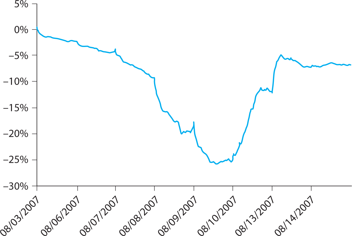
Figure 9.6. The quant equity event of August 2007.
The graph shows the simulated cumulative return to a long-short market-neutral value and momentum strategy for U.S. large-cap stocks, scaled to 6% annualized volatility during the period August 3–14, 2007.
Source: Pedersen (2009).
On Monday, August 6, 2007, a major deleveraging of quant strategies began. Figure 9.6 shows a simulated cumulative return to an industry-neutral long–short portfolio based on value and momentum signals. As discussed above, fundamental quants also use many other factors, and not all were affected, but many have some exposure to value and momentum. Also, certain statistical arbitrage strategies that rely on price reversals were affected by the liquidity event due to the unusual amount of price continuation (not shown in the graph).
The figure shows that the portfolio incurs substantial losses from Monday, August 6, through Thursday, August 9, as quants were unwinding, and then recovers much of its losses on Friday and Monday as the unwinding ended and some traders may have reentered their positions. The smoothness of the graph is noteworthy. It is not an artifact of drawing the graph by connecting a few dots—the graph uses minute-by-minute data. The smoothness is due to a remarkable short-term predictability arising from the selling pressure and subsequent snapback. For instance, the strategy was down 90% of the ten-minute intervals on Tuesday, August 7. This predictability provides strong evidence of a liquidity event, as it is statistically significantly different from the behavior of a random walk.
Notice the magnitude of the losses in figure 9.6. The simulated strategy loses about 25% from Monday to Thursday, and it has been scaled to have an annualized volatility of about 6% using a well-known commercial risk model. If you interpret this volatility naïvely, it means that the strategy should, with a certain confidence, be able to lose up to about 12% in a year. In this event, it lost twice that in just four days!
Considering the four-day volatility of 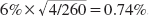 , the strategy’s loss is more than thirty standard deviations. The thirty standard deviations must be interpreted correctly. This number does not mean that this was a thousand-year flood and can never happen again. It means that the event was a liquidity event, not based on stock fundamentals, and that this risk model does not capture liquidity risk and the endogenous amplification by the liquidity spirals. Indeed, most of the time stock price fluctuations are driven primarily by economic news about fundamentals, but during a liquidity crisis, price pressure can have a large effect. Hence, the distribution of stock returns can be seen as a mixture of two distributions: shocks driven by fundamentals mixed with shocks driven by liquidity effects. Since fundamentals are usually the main driver, conventional risk models are calibrated to capture fundamental shocks, and liquidity tail events are not well captured by such models. Hence, the result of 30 standard deviations means that the event is statistically significantly different from a fundamental shock and, hence, must have been driven by a liquidity event.
What do you do when you are in the middle of a liquidity spiral? Well, first you must figure out whether your losses are indeed due to a liquidity spiral or fundamental losses. The difference is important because a liquidity spiral eventually ends, most likely with a snapback, whereas fundamental losses might continue and have no reason to be reversed. Figure 5.6 in chapter 5 shows a stylized price path during a liquidity spiral when everyone is running for the exits and prices drop and rebound (based on a model that I had published two years before the quant event with Markus Brunnermeier).6 There is a striking similarity between the stylized figure 5.6 and the plot of actual market prices in figure 9.6: Both graphs go down smoothly, go back up smoothly, and, finally, level off below where they started. This drop and rebound in prices is the signature of a liquidity spiral, a signature that is also seen in many other liquidity events, such as the flash crash discussed later.
Clearly, the quant event was a liquidity spiral when considering all the evidence until Thursday (see the calculation above), but when did this become clear? Well, in real life nothing is ever crystal clear except with hindsight, but quants had a good idea already on Monday. First, the losses seemed too large and too smooth during the day to be explained by other factors. Second, while there were fundamental drivers of losses for value investing in July, the total losses of value plus momentum were becoming hard to explain and now economic fundamentals seemed to be improving for the stocks that were held long relative to the stocks that were shorted in this portfolio. In fact, while the simulated portfolio was losing enormous sums, equity analysts were upgrading their recommendations of its long positions relative to its shorts, again suggesting that the losses were liquidity driven, not due to fundamentally bad bets. Third, the co-movements across stocks behaved anomalously and also suggested a liquidity spiral. For instance, even though momentum is normally negatively correlated to value, these strategies suddenly became positively correlated. Said differently, stocks started moving in sync just because they might be held by quants even if they were not fundamentally linked. Fourth, the events this Monday followed other alarms bells that had already started ringing in July and the first week of August.
Having identified a liquidity spiral, what should you do? You have several options: (a) partially liquidate the portfolio, which frees up cash, reduces risk, but contributes to the adverse price moves, incurs transaction costs, and gives up part of the upside when the liquidity spiral turns; (b) rotate the portfolio toward the more idiosyncratic factors that were not affected by the unwinding, which would also incur transaction costs, give up upside, but not free up any cash; (c) stay the course; (d) add to the position, betting that the turnaround is near; or (e) not just liquidate the portfolio but also flip it around, incurring large transaction costs in a big bet that the unwinding would continue for a long time and a bet that goes against all the factors that you normally believe in.
Different quants took different strategies, and the best action depended on the leverage of the fund, the financing of the leverage (including the margin requirements and the risk that the margin requirements would change), the amount of free cash, the risk of the portfolio, and the size and liquidity of the portfolio. An unleveraged long-only stock portfolio faces no risk of forced liquidation by creditors (however, investors might redeem their assets, but this tends to happen more slowly), so such portfolios can better wait out the crisis or even add to the exposure of the most affected factors. In contrast, a highly leveraged portfolio cannot sustain large losses without managing the risk and therefore you need to carefully reduce positions and free up cash to avoid getting a margin call and avoid doing so too late. With larger and more illiquid portfolios, you must take into account that such risk management takes more time. When you see that the liquidation is about to end, you must be ready to quickly increase the position to earn as much of the reversal as possible. Indeed, as seen in figure 9.7, the portfolio finally raged back the other way on Friday, making enormous sums of money and profiting about three-quarters of the day’s ten-minute intervals.
It is important to remember that the quant event happened during a relatively calm period for the overall stock market. The stock market was up 1.5% during the week of the quant event, and it was up year-to-date through July and August. Hence, the quant event was hidden from the general market because it could only be seen through the lens of a quant portfolio.
Figure 9.7. Deviation from parity for Unilever’s dual-listed stocks.
The figure shows the percentage spread between the prices of Unilever NV and Unilever PLC computed as PNV/PPLC – 1, where the adjusted prices are expressed in common currency.
In 2008, the liquidity problems spread much more broadly around the economy and, in September 2008 a truly systemic liquidity crisis unfolded around the bankruptcy of Lehman Brothers. Ironically, the value/momentum quant equity strategies performed relatively well during 2008.
9.2. STATISTICAL ARBITRAGE
Statistical arbitrage (stat arb) strategies are also quantitative, but they are usually less based on an analysis of economic fundamentals and more based on arbitrage relations and statistical relations.
Dual-Listed Shares: Siamese Twin Stocks
Some stocks are joined at the hip in the sense that their fundamental values are economically linked. A classic example is when two merging companies in different countries decide to retain separate legal identities but function economically as a single firm through an “equalization agreement.” The merged entity has dual-listed shares in the sense that both its former shares continue to be listed on the respective exchanges.
For instance, the Unilever Group originated from the 1930 merger of the Dutch Margarine Unie and the British Lever Brothers. Unilever still consists of two different companies, Unilever NV, which is based in the Netherlands and has shares traded in euros, and Unilever PLC, which is based in the United Kingdom and has its shares traded in British pounds at the London Stock Exchange. While the prices of NV and PLC follow each other closely, there is often a significant spread between the two, as seen in figure 9.7.
In globally integrated and efficient financial markets, the stock prices of the twin pair should move in lockstep and always be at parity. In practice, however, there are deviations from parity, as seen for Unilever and other twin stocks. Each stock moves partly with its own market.
Multiple Share Classes
Another stat arb trade based on closely linked securities arises when the same firm issues different share classes, such as A shares vs. B shares or ordinary shares vs. preference shares. Often B shares have fewer voting rights than A shares but the same rights to dividends. Similarly, preference shares may have the same rights to payments but fewer control rights (although preference shares are often debtlike securities). Furthermore, there is sometimes a significant difference in the liquidity in the different share classes. The differences in voting right and liquidity can lead to very significant spreads between the share classes. For example, figure 9.8 shows the price discount of BMW’s preference shares relative to the regular shares, a discount that varies over time and has been large for long time periods.
Trading on the spread across share classes is not a perfect arbitrage, not just because the spread can widen but also because corporate events can lead to a different treatment of the different share classes. For instance, an activist investor might propose corporate actions that affect the share classes differently, e.g., differential share repurchases. On the other hand, many corporate events can also lead to a collapse of the spread, e.g., this may happen if the company is taken over.
Figure 9.8. The price discount of BMW preference shares relative to the ordinary shares.
Efficiently Inefficient Arbitrage Spreads: The Case of Twin Stocks
Stat arb traders trade on the discrepancy between twin stocks. This practice reduces the arbitrage spreads, but competition between stat arb traders often does not entirely eliminate the spread. Trading on these spreads requires a constant monitoring of the market from identifying mispricing in the first place, understanding the contractual rights of the different types of shares, and executing the trade. The trade execution involves transaction costs and often currency risk that needs to be hedged.
The arbitrage spread would be zero in a perfectly efficient market, so non-zero spreads provide clear evidence of market inefficiencies. The spreads are efficiently inefficient, however, in the sense that spreads are larger when the arbitrage trade is riskier and more costly to implement and when arbitrage capital is more scarce. As a further sign of efficiently inefficient pricing of liquidity risk, it is often the less liquid shares that trade at discounts, particularly when the liquidity premium is high.
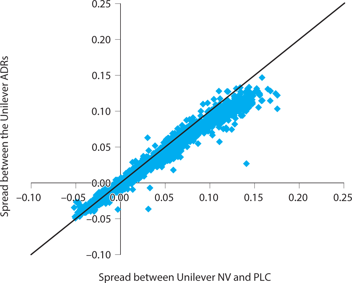
As an example of the efficiently inefficient market, consider the arbitrage spreads between local Unilever shares trading in Europe relative to their counterparts trading in the United States as American depositary receipts (ADRs). The ADR for Unilever NV trades very close to the actual price of the NV, often within 0–2% (depending on how well you synchronize the prices) and, similarly, the ADR for Unilever PLC trades very close to the actual price of PLC. However, the ADR trades at significant spreads to each other, just as the ordinary NV and PLC shares do. Why is this?
The ADRs trade at close prices to the regular shares because the arbitrage spread reflects a relatively simple arbitrage. This is because the ADR and the ordinary shares are fungible in the sense that one can be exchanged for the other (similar to the way in which exchange traded funds (ETFs) can be created and redeemed). In contrast, if you buy a share of NV and short a share of PLC, these positions cannot be netted—you must hold both positions until their prices converge, potentially tying up capital for a long time.
The arbitrage spread between the ADRs closely follows the arbitrage spread of the ordinary shares. However, as seen in figure 9.9, the spread tends to be slightly smaller for the ADRs. This difference is likely because the ADR arbitrage is a slightly simpler strategy since both ADRs are traded in U.S. dollars, so no currency hedging is needed. The smaller ADR spread thus represents another sign of efficiently inefficient markets.
Figure 9.9. The arbitrage spreads of ADRs vs. the local shares of Unilever.
The horizontal axis shows the arbitrage spread of the ordinary shares of Unilever NV vs. PLC, and the vertical axis shows the arbitrage spread of the corresponding ADRs, 2000–2013. The graph also shows the 45-degree line. The fact that most points lie between the horizontal axis and the 45-degree line reflects that the ADR spread tends to be smaller since it corresponds to an easier arbitrage.
Pairs Trading and Reversal Strategies
In addition to finding dual-listed stocks and closely related share classes, stat arb traders also look for stocks that simply behave similarly in a statistical sense without any explicit arbitrage link.7 One such strategy is pairs trading, where stat arb traders look for pairs of highly correlated stocks, identify situations when their prices move apart, and bet on a convergence by buying the stock that lags behind and shorting the one rising more.
Pairs trading is a bet on price reversals. Stat arb traders also make broader bets on price reversals. Such broader reversal strategies do not consider pairs of stocks but simultaneously consider a larger universe of stocks and seek to buy those that lag behind and those that have gotten ahead of the market. The simplest type of reversal strategy is to buy stocks that have experienced the lowest return over the past days and short those that had the highest return. More sophisticated reversal strategies (also called residual reversal strategies) seek to estimate each stock’s expected return in light of its characteristics and the returns of other stocks with similar characteristics, and then bet that the residual between the stock’s actual return and its expected return will revert.
Index Arbitrage and Closed-End Fund Arbitrage
Finally, stat arb traders pursue strategies that seek to arbitrage the difference between a “basket security” and its components. For example, they try to arbitrage the difference between stock index futures and the prices of the underlying stocks, the discrepancies between futures and an ETF, the difference between the ETF and its constituents, and the difference between a closed-end mutual fund and its underlying stock holdings. These arbitrage spreads tend to be small given that the strategies can be implemented with limited risk, with the exception of the closed-end funds, where large arbitrage spreads can arise. These trades often require very sophisticated trading infrastructure to minimize the transaction costs and limit execution risk, given the many legs of the trade as well as minimal funding costs if spreads are tight.
9.3. HIGH-FREQUENCY TRADING: EFFICIENTLY INEFFICIENT MARKET MAKING
HFTs trade many different strategies; some provide liquidity, and others demand liquidity.8 When HFTs provide liquidity in today’s electronic markets, they essentially serve the same role as the old-fashioned market makers and the specialists on the floor of the New York Stock Exchange.
Liquidity would be almost unlimited and bid–ask spreads virtually zero in a perfectly efficient market in which all investors are always present in the market and have the same information. However, as we have seen, markets are not perfectly efficient and liquidity problems are everywhere. To understand the basic economics of market making in an efficiently inefficient market, note that most investors do not follow the markets constantly, they occasionally decide to trade, and then they often want to trade immediately. Hence, the natural buyers and the natural sellers do not arrive in the market at the same time and, even when they do, they sometimes go to different exchanges, so the order flow is fragmented. This behavior means that the market price bounces around the “equilibrium price” (that is, the price that would prevail if all the buyers and sellers were present in the market simultaneously) and the price would bounce around a lot more if it weren’t for the market makers (and here I am using the term “market makers” generally, including liquidity-providing HFTs). That is, when an excess of buyers show up in the market, the price is pushed up, and when the sellers show up, the price is pushed down.
Market makers provide a service, namely liquidity (or immediacy). That is, when more sellers arrive to the market than buyers, market makers stand ready to buy the excess supply. Market makers hold the securities in inventory until the natural buyers arrive, satisfying the buyers’ demand by unloading the inventory.
Market makers charge a price for the liquidity service. This price is the profit of the market maker and the transaction cost of the natural buyers and sellers. Specifically, market makers earn profits due to the bid–ask spread and due to market impact, i.e., buying low and selling high as the price bounces around. This is similar to the profits earned by a grocery store with a markup between what it pays for the groceries and what it sells them for. The grocery store needs to earn a markup large enough to be compensated for paying its employees, rent, freight costs, and the cost of capital, but in a competitive market, the markup should be no greater than that. Similarly, market makers need compensation for the costs associated with liquidity provision and, the more competitive the market, the more liquid the market.
In addition to the costs of setting up a large trading infrastructure, market makers face the risk of losing money because they are trading against informed investors. Indeed, if there is selling pressure in the market (leading the market makers to be net buyers), this could either be because of order fragmentation or because the equilibrium price has actually changed—and market makers are never sure which one it is. In the former case, market makers buy low and then sell high when the price rebounds, earning a profit. In the latter case, market makers buy low and sell even lower when they realize that the price pressure was not a temporary effect but rather an expression that the fundamental value has declined (and sellers might have known something that the market maker didn’t know). Hence, to be profitable, market makers need to keep adjusting to the market conditions. When news arrives, they need to immediately adjust their orders. Indeed, limit orders provide the market with free “options” to trade whenever the true value has changed.
Conceptually, market makers in electronic markets work as follows. They seek to determine the equilibrium price of a stock and submit a limit order to buy at a price just below the equilibrium price and a limit order to sell at a price just above it. They constantly update their estimates of the optimal order placement based on other orders arriving to the market for this stock and other stocks, and then they frequently cancel orders when the equilibrium price changes and submit new ones. Furthermore, market makers must manage inventory risk, making sure to shade orders to encourage the market to diminish their positions and hedge market and industry exposures.
HFT also pursues many other strategies than liquidity provision and, in fact, by some estimates they initiate trade with marketable orders more often than their limit orders are hit passively. For example, HFTs exploit short-lived relative mispricing across related securities similar to the stat arb strategies discussed above. Some HFTs also have strategies that seek to hit “stale” limit orders, including the limit orders submitted by other HFTs. For instance, if a news announcement increases the value of a stock, the HFT will immediately hit (i.e., buy from) a limit order to sell near the old equilibrium price. Simultaneously, liquidity-providing HFTs immediately try to cancel their stale orders.
HFTs engage in an “arms race” against each other where being fast is not important per se but being faster is very important. Indeed, there are only so many stale limit orders, so only the fastest HFTs get to hit them. On the flip side, to reduce the risk of being exposed to adverse selection, an HFT needs to be able to cancel its own limit orders before they become stale and are hit by other HFTs.
Some HFTs may also try to identify and exploit large orders that are broken up into smaller trades and traded over hours or days. For example, if you are seeking to buy a large stock position, try to submit a limit order to buy the same number of shares each minute, right at the minute, and see what happens to your execution (relative to an execution where you split up the order more finely and more randomly and execute at more random times).
The Flash Crash of 2010
On May 6, 2010, dramatic market events occurred in the U.S. stock market that came to be known as the flash crash. From the morning, the market was dropping on large trading volume and volatility due to rising fears about the ongoing European debt crisis.
At 2:32 p.m., the Standard & Poor’s 500 (S&P 500) stock market index was down 2.8%. The limit order book was thinning due to the heightened volatility and because some exchanges were experiencing data delays and other data problems. When traders in electronic markets start to question the data quality, it is as if they cannot “see,” and being afraid to trade blindly, they naturally scale back their orders or even pause trading altogether.
At this time, a mutual fund (reportedly, Waddell & Reed Financial, Inc.) submitted a very large order to sell 75,000 e-mini S&P 500 futures (about $4.1 billion worth). Such a large order rarely hits the market; in fact, it had only happened twice over the previous 12 months, one of which was by the same mutual fund. The last time this mutual fund had executed a similar sized order, it had done so over the course of several hours, but on the day of the flash crash, the selling mutual fund decided to have the order executed with an algorithm over just 20 minutes. Over the next 13 minutes, the market dropped 5.2% in value, an enormous move over such a short time period, as seen in figure 9.10.
HFTs initially provided liquidity. They were net buyers as the market was dropping, but, at 2:41 p.m., HFTs turned around and became net sellers, perhaps to reduce their inventory risk, but throughout the event, HFTs were mainly buying and selling to each other as documented by the CFTC and SEC:
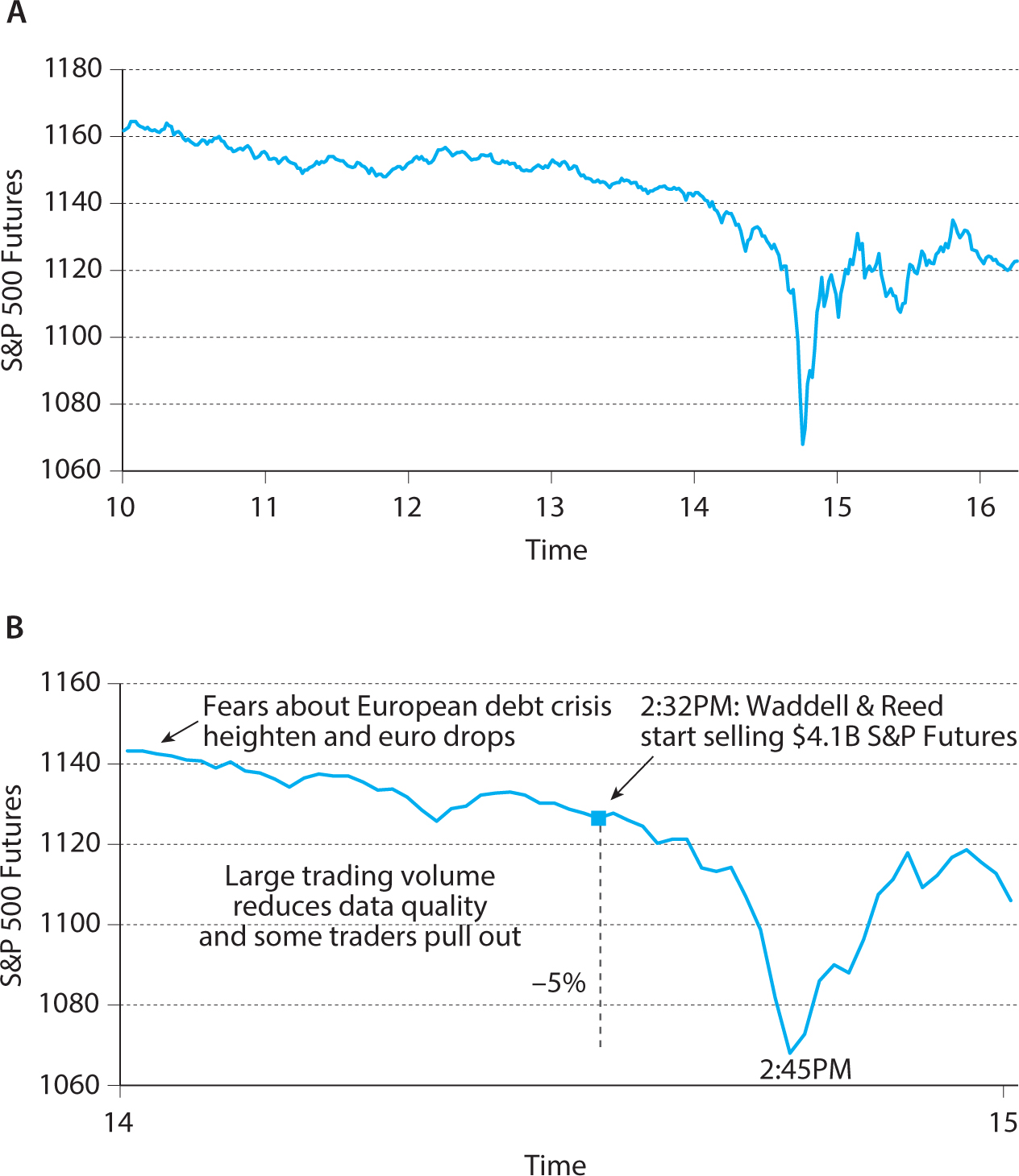
Figure 9.10. The flash crash of May 6, 2010.
Still lacking sufficient demand from fundamental buyers or cross-market arbitrageurs, HFTs began to quickly buy and then resell contracts to each other—generating a “hot-potato” volume effect as the same positions were rapidly passed back and forth. Between 2:45:13 and 2:45:27, HFTs traded over 27,000 contracts, which accounted for about 49 percent of the total trading volume, while buying only about 200 additional contracts net.9
CFTC and SEC continues:
At 2:45:28 p.m., trading on the E-Mini was paused for five seconds when the Chicago Mercantile Exchange (“CME”) Stop Logic Functionality was triggered in order to prevent a cascade of further price declines. In that short period of time, sell-side pressure in the E-Mini was partly alleviated and buy-side interest increased. When trading resumed at 2:45:33 p.m., prices stabilized and shortly thereafter, the E-Mini began to recover.
When the price of the S&P 500 neared the bottom, its liquidity dried up in the sense that the depth in limit order book almost completely vanished. Furthermore, the liquidity crisis in the S&P 500 spilled over to many other markets, partly because traders were arbitraging the relative mispricings that arose due to the falling S&P 500. Relative-value traders started buying the S&P 500 while shorting other securities, thus depressing prices in other markets (while supporting the S&P 500). First, ETFs were hit, and then many individual stocks. Some stocks experienced highly unusual trades as their limit order books were wiped out, and market orders started hitting “placeholder bids” at extreme prices, including a trade at $0.01 for Accenture. The most extreme trades were later canceled, however.
The role of HFTs in the flash crash was not so much what they did but what they didn’t do, namely provide unlimited liquidity. However, the failure of market makers to provide liquidity in the face of overwhelming one-sided demand pressure, confusion about market prices, and increasing risk has always been a problem. For example, old-fashioned market makers in NASDAQ stocks and in over-the-counter markets have been known to take their phones off the hook when markets have gone off the cliff, e.g., in the 1987 stock market crash. Also, half a century before the flash crash of 2010, a similar event occurred that came to be known as the “Market Break of May 1962.” This event was also investigated by the SEC and, as in the flash crash, the SEC found that the “lateness of the NYSE tape and the size of the price declines on the NYSE prompted some over-the-counter dealers to withdraw as market makers in certain securities.”10
9.4. INTERVIEW WITH CLIFF ASNESS OF AQR CAPITAL MANAGEMENT
Cliff Asness is a cofounder and managing principal at AQR Capital Management, a global investment management firm built at the intersection of financial theory and practical application. One of the original quant investors, Asness has also written a large number of influential and award-winning articles. Before cofounding AQR, he was a managing director and director of quantitative research at Goldman Sachs Asset Management. He earned two B.S. degrees from the University of Pennsylvania and his Ph.D. and MBA from the University of Chicago, where he wrote his dissertation, one of the very early studies of momentum investing, establishing the type of momentum strategy still most commonly studied in academia today, as Prof. Fama’s student and teaching assistant.
LHP: Your Ph.D. dissertation had seminal research on momentum, reversal, and statistical arbitrage—how did that come about?
CSA: Being present at the University of Chicago when my two advisors, Gene Fama and Ken French, were doing their research on value and size, I first thought I would write some extension of value investing. I spent a lot of time with the data, and I kind of ran across this weird result that stock returns have strong momentum (measured over the last twelve months, leaving off the most recent month). The momentum effect was about as strong as value investing, in fact, even stronger in gross returns. I hadn’t seen this result in the academic literature (though it turned out that two researchers at UCLA were looking at something similar at the same time, minus that skipping the last month part), so I was pretty excited, but also nervous. Gene was a big believer in efficient markets, so the thought that I would write a thesis for him on something that was on the surface so inconsistent with market efficiency was a bit scary. I recall telling him about these findings, fully expecting him to send me back to the drawing board, but his response was “If it is in the data, pursue it!” That was a great moment for me and my respect for Gene.
Another thing I found while mucking around with the data was that the most recent month was associated with reversal. I thought that was cool, but I wasn’t fully sure how implementable it was. It turns out that effect was the seeds of what many successful stat arb traders have been able to build around, and I gave up on it too soon. It is my personal “fish story,” that is, the one that got away …
LHP: Was there a moment when you realized that your momentum result was a significant finding?
CSA: For me, probably the key moment in my dissertation was when I extended the sample back to 1926. As you know, the only cure for data mining is an out-of-sample test, so I wanted to see if my findings held up during another time period. I was initially doing all my analysis using the same data as Fama–French from 1963 to 1990, but it suddenly dawned on me that there existed data from 1926. Fama–French only used data starting in 1963 because they didn’t have companies’ book values earlier than that. This is really obvious, but I just said, “Wait a second. I do have price data from 1926, and unlike them my stuff doesn’t need book values, so why am I limiting myself to their sample period?” So I basically ran my stuff from ’26 to June of ’63. This became one of the “famous regressions in my life”; yes, I know not many people have that category (and it’s only famous to me). It just worked perfectly on pristine data that hadn’t been looked at yet. The momentum effect was strong, the most recent month’s strong reversal was there, and the longer term reversal also worked pre-1963. That was a very exciting moment for me as a twenty-three-year-old. I was like, “Holy crap, it works!” That said, I had no idea momentum would play such a large role in academia. I just wanted to graduate.
LHP: When I was in graduate school at Stanford, my professors discouraged internships on Wall Street, referring to the tragedy that happened to Chicago, where their best Ph.D. students left academia, following a “corrupting” star student to go to Wall Street. I think it’s been called Chicago’s “lost generation.” Can you tell me about that?
CSA: Ha! Well, for many years afterwards, I kept hearing from my academic friends that Gene was mad at me for leaving academia. I guess it made it worse that a whole bunch of my Chicago Ph.D. classmates came with me when I left. My response was always, “Really???” and their response was, “No, not really….” Well, Gene trained me to be a good empiricist, so after this happened enough times I realized there was probably something to it. But I always tried to think of it as a compliment, and Gene and I are on very good terms today.
LHP: So, why did you decide to leave for Wall Street?
CSA: I absolutely loved the work that I was doing when I was at Chicago. But I went to graduate school straight from college, so I have to admit that I did have a little nagging question about what the real world would be like. Also, my best friend from college went to Goldman Sachs and was telling me that I owe it to myself to at least see what it’s like. So I decided to try a summer at Goldman. It turns out that summer never ended! I started out as a fixed-income trader. So by day I traded bonds, and by night I worked on my thesis, which was on stocks. After a short time, Goldman decided it needed a quantitative research group that covered both stocks and bonds, and they asked me to start that up. The mandate for the group was quite broad, and it struck me that here was an opportunity for me to be able to do all the fascinating things I was working on in school, and I would work with the rigor of an academic, but in a more applied setting. That was really appealing to me.
LHP: What were the most difficult steps in the transition from studying markets academically to using the research to trade real money?
CSA: First, there was learning how the real world works, all the broker relationships, and so on. Then you quickly see the importance of transaction costs and portfolio construction. It’s not that academics don’t know about these things, but when you’re doing it for real money, playing with “live ammunition” as they say, it ups the ante. For instance, you realize that, if you want to run a reasonably large amount of money, you can’t go as deep into small cap as you’d like, where transaction costs are too large. You can’t run a very high turnover strategy, etc. Also, one of the biggest adjustments was having to convince people that you can really do it. I will tell you the hurdle for people letting you play with live ammo, their ammo, can be very different from the hurdle to writing a successful paper. I was a twenty-five-year-old geek at Goldman Sachs, saying, “Give me money; this quant stuff seems to work.” For example, they made us go present our work to Abby Cohen the then, and still, Goldman markets guru. I respect Abby, but she was a very different kind of analyst than we were. But we did it, she got it, and gave us the thumbs up.
LHP: What else is different in the real world?
CSA: Well, the single biggest difference between real world and academia is—this sounds over scientific—time dilation. I’ll explain what I mean. This is not relativistic time dilation as the only time I move at speeds near light is when there is pizza involved. But to borrow the term, your sense of time does change when you are running real money. Suppose you look at a cumulative return of a strategy with a Sharpe ratio of 0.7 and see a three-year period with poor performance. It does not faze you one drop. You go: “Oh, look, that happened in 1973, but it came back by 1976, and that’s what a 0.7 Sharpe ratio does.” But living through those periods takes—subjectively, and in wear and tear on your internal organs—many times the actual time it really lasts. If you have a three-year period where something doesn’t work, it ages you a decade. You face an immense pressure to change your models, you have bosses or clients who lose faith, and I cannot explain the amount of discipline that you need.
LHP: Warren Buffett’s Berkshire Hathaway stock return has a Sharpe ratio of about that magnitude.
CSA: Yes, and he had some periods of losses too, of course—some of them fairly horrific. A Sharpe ratio of 0.7 can make a lot of wealth, but it still loses a fair amount of times and sometimes for multiple years in a row. I got lucky—this is probably the single biggest luck in my professional life, that the first couple of years were very good for our process. We made a lot of money in the first two years with great risk-adjusted returns. If the first couple of years were bad, I’d probably be doing something else; that’s just how this business works. It’s a good process, and it has worked over time, including the full “out of sample period” since my dissertation ended, so I don’t feel this piece of good luck was at all unfair (of course I don’t!), but navigating through the inevitable bad times is the single biggest change of mind-set you have to make leaving academia.
LHP: Yes, when you started your quant group at Goldman Sachs, you were a young guy with triple digit returns, on track to become a Goldman Sachs partner—so why did you walk away from that to start a new firm?
CSA: That wasn’t an easy decision. We were doing well at Goldman, and they treated us great. But if you projected forward, the path at Goldman would be very different than the path as an independent firm. For me, success would increasingly look like becoming more a part of senior management at a very large firm. The path on our own might keep me closer to research, which has always been my passion. A couple of catalysts pushed me to make the decision. One was that a fellow Chicago Ph.D. classmate who worked for me at the time left to start his own hedge fund, and his initial success got my competitive juices flowing. Second, a Goldman colleague from another group, David Kabiller, also started making the case that we could successfully do this on our own. He almost had more confidence in us than we did—and lots of business ideas. So a year later, I left with John Liew and Bob Krail (also fellow Chicago Ph.D. classmates and the two most senior members of my team), about half the rest of the team in total, and David to start AQR. I should say the people who stayed at Goldman to run our old group were an all-star team themselves, too.
LHP: So you decided to take the chance and start AQR.
CSA: Yes, we had an easier time raising money than we expected and in fact had to turn back about half of the subscriptions. However, we had no idea what was coming around the corner. Those young and cocky Goldman Sachs quants were about to eat humble pie for a long stretch!
LHP: You are referring to the tech bubble?
CSA: Correct. Actually, our first month, August 1998, was good despite that the market was collapsing and LTCM and many other hedge funds were getting into trouble. We were running very different strategies, and we made money. Then things turned south. To understand why, recall that two very important investment themes underlying our trading strategies are value and momentum—we used other strategies too and have developed many new ones over the years, but these are still important. The tech bubble was a period when value was strongly out of favor and momentum helped, but not nearly enough. It turns out we timed the launch of our business and our first fund right before the start of the tech bubble, literally just before the start of its really crazy phase. Remember the idea behind time dilation I mentioned before? Our tough start lasted about 18 months, but it felt like a lifetime.
LHP: How did investors react to the tough start?
CSA: Many of our investors stuck with us, especially those who really understood our process, and we showed them lots of evidence that the Internet valuations didn’t make sense and that, going forward, our investments looked even better. Of course, while many did, not every investor stuck with us. One of the frustrating things about this business is how sensitive many investors are to short-term performance—in both directions, we’ve been the beneficiaries also. Many investors have a tendency to pile into investment strategies or managers who have recently had good performance, and they flee at the first sign of trouble, or, even worse, stick around a bit and get out at the worst possible time when it feels like it’s been losing forever, but statistically it’s not even that shocking. The problem with this behavior is that, if you poorly time the entry and exit of these strategies, you are not able to take advantage of the fact that these strategies make money over the long run. I shouldn’t whine too much; it’s probably why some of the strategies exist in the first place and don’t get arbitraged away as easily as some might assume, but it’s hard to keep that perspective at times. In any case, the investors who stuck with us really got rewarded when the Internet bubble burst in 2000 and the following years.
LHP: Let’s shift gears a bit and talk about your approach to quantitative investments. So how do you pick stocks?
CSA: Well, everyone has secrets, but I’ll share a few of the most basic ideas: As I mentioned before, at the simplest level and leaving out a fair amount, we’re looking for cheap stocks that are getting better, the academic ideas of value and momentum, and to short the opposite, expensive stocks that are getting worse. Our models are a lot subtler than that today, including other themes, and more sophisticated ways to ferret out cheapness and momentum, but while we’ve been striving to improve things for a long time now, the core principles remain the same after 20 years.
Further, while my dissertation was on equities, we extended the research to bonds (remember, I was a bond trader), currencies, commodities, and several other asset classes.
LHP: What are the differences/similarities between quantitative and discretionary investment?
CSA: I think good judgmental managers are often looking for the same things we are—cheap stocks with a catalyst as to why they won’t remain cheap, and vice versa for shorts. In fact, for a long time I used to think we did something very different, until I realized that “catalyst” and “momentum” share a lot in common and so do quants and more discretionary managers. In fact, be it for rational or irrational reasons, I think this is the type of management, quant or judgmental, that adds value over time. The big difference between quants and non-quants comes down to diversification, which quants rely on, and concentration, which judgmental managers rely on. But what we tend to like or dislike in general is actually fairly similar.
A discretionary manager gets to intimately know the companies they invest in. We don’t, but our advantage is that we can apply our trading philosophy to thousands of stocks at the same time. If the philosophy works, it’s very hard for us to lose over time given that we spread the risk over so many stocks. Of course, as implied earlier, it’s very easy to lose for a while even if you’re right! Even if a discretionary manager knows a company very well, the CEO can still turn out to be a philandering embezzler, so you have that stock-specific randomness if you only hold a few stocks. And no matter how well you know something, there is still just a chance you’re wrong.
LHP: What are the main benefits of quant investment?
CSA: Quantitative investors can process a lot of information. We look at many more stocks and many more factors than is easily done by discretionary stock pickers. Further, we apply the same investment principles across stocks, backtest our strategies, and follow our models with some discipline.
LHP: Do you always follow the models?
CSA: Discipline is important. We do not think we’re more immune to psychological biases than others, but following the models helps. If we followed them with less discipline, we run the serious risk of reintroducing the exact biases we are trying to exploit! For instance, if people run from stocks with any problems, making value stocks too cheap and attractive buys long-term, if we use our judgment to selectively override our models, perhaps we undo precisely the bet we want to make, in order to make ourselves more “comfortable”? Discipline is not always easy, by the way. It’s really hard to stick to a strategy. But when people cave and disregard their models, they seem to usually do this within an hour and a half of the worst possible time to cave. Admittedly, that’s not a quant study, but it’s been my experience. The difficulty of sticking to the models is part of why they work.
LHP: How do you determine whether a new trading factor is good?
CSA: We have a lot of trading factors, as you know, ranging from a number of more sophisticated value and momentum factors to factors based on altogether different signals. We’ve been working on this for 20 years, and all the additions and changes to our model had to pass a number of tests. First, it has to make some sense. Then, unlike a judgmental manager, we have to test it. It has to survive a number of out-of-sample tests. For instance, does a trading signal work in all countries? Across time periods? Does it work after the time when it was first discovered? If applicable, does it work in different asset classes? Also, we test the economics of the idea, not just the return performance. If the idea is that a factor predicts earnings and therefore returns, we test whether it in fact does predict earnings, not just returns. We also focus keenly on whether the performance survives transactions costs.
LHP: In your view, what are the main reasons that these strategies work?
CSA: You know, there are three possible reasons a strategy may have worked in the past: One is random chance. I don’t believe that’s it (I better not!). I think we’re fairly rigorous, and we’ve tested our stuff in a hundred places including 20 years out of sample from when first discovered. So for our core strategies at least, I’m very certain it is not just random chance, but you still have to list that as a possibility; not to is just intellectually dishonest. Two is that our strategies may work because we’re picking up a risk premium: What we are long is riskier than what was short, and we’re getting paid for that. The last possibility is that what we’re doing is something that is a bit of a free lunch, that is, a market inefficiency brought on presumably by other investors acting irrationally or with a “behavioral bias.” Frankly, over time, I drifted more toward the latter, but not as far as most of the active management world. Free lunch, by the way, sounds too great since you still have to work really hard to collect it using sophisticated portfolio optimization techniques and suffer through those periods where it doesn’t work for a while. So I think in some places we’re picking up disciplined risk premiums that are not very correlated with long-only markets, which means, if someone doesn’t have those in their portfolio, they should add them. In other places, I think we’re taking advantages of human biases and we’re trying to be disciplined and determined about it, taking the other side of some common psychological trait or institutional constraint that influence security prices.
___________________
1 Studies of the relation between book to market and expected returns go back to Stattman (1980). An even simpler measure of value is the return over the past five years, where value stocks are taken to be those with a low past five-year return (De Bondt and Thaler 1985).
2 Fama and French (1993) construct such long–short portfolios separately among small and large stocks, respectively, and then take the average of these two portfolios. This construction seeks to reduce size effects in the HML factor.
3 Momentum profits were first documented by Jegadeesh and Titman (1993) and Asness (1994). Theories of initial underreaction and delayed overreaction have been proposed by Barberis, Shleifer, and Vishny (1998), Daniel, Hirshleifer, and Subrahmanyam (1998), and Hong and Stein (1999). For more on the relation to catalysts, see the interview with Cliff Asness in this chapter.
4 The flat security market line was first documented by Black, Jensen, and Scholes (1972). The idea that leverage constraints can explain this phenomenon was pioneered by Black (1972, 1992) and extended by Frazzini and Pedersen (2014), who found evidence in several asset classes and in the portfolios of mutual funds, individuals, Warren Buffett, and LBO deals. Asness, Frazzini, and Pedersen (2014) studied BAB factors within and across industries. Clarke, de Silva, and Thorley (2013) consider other forms of low-risk investment.
5 This section is based closely on Pedersen (2009). See also Khandani and Lo (2011).
6 Brunnermeier and Pedersen (2005, 2009).
7 See Gatev, Goetzmann, and Rouwenhorst (2006) for pairs trading and Nagel (2012) on reversal trades and their relation to liquidity and volatility.
8 Jones (2013) provides an overview of HFT, a review of the flash crash, and a list of relevant references. Budish, Cramton, and Shim (2013) analyze the HFT trading arms race.
9 U.S. Commodities and Futures Trading Commission and Securities and Exchange Commission (2010).
10 U.S. Securities and Exchange Commission (1963).