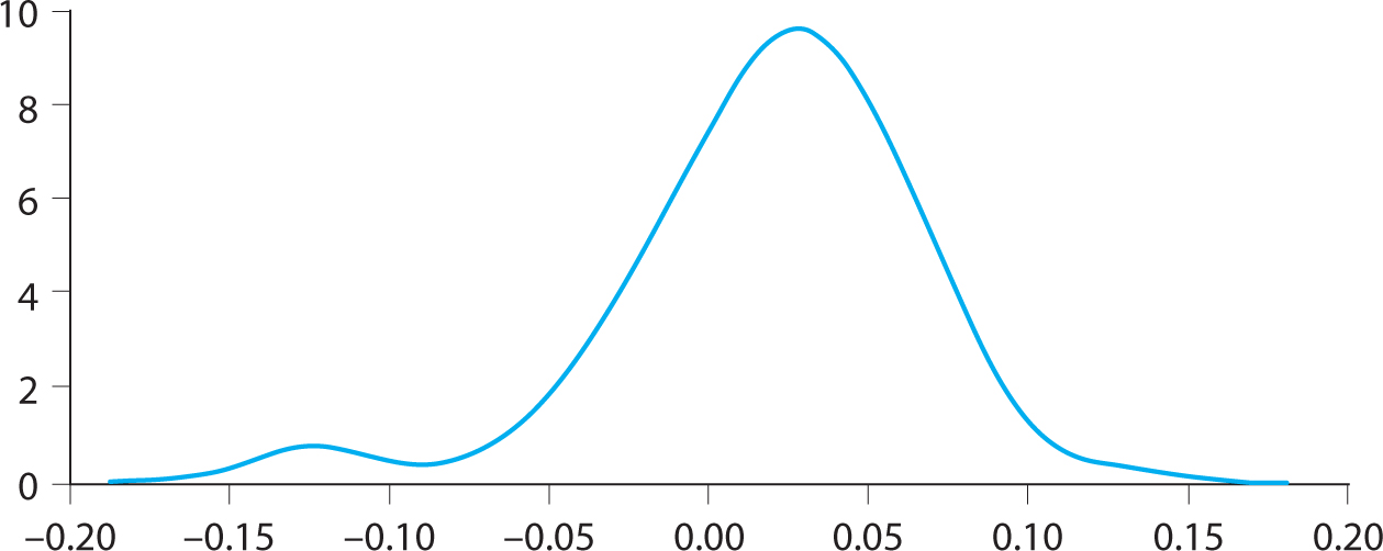
Figure 11.1. The distribution of quarterly excess returns from the currency carry trade.
Source: Brunnermeier, Nagel, and Pedersen (2008).
Global Macro Investing
The whole world is simply nothing more than a flow chart for capital.
—Paul Tudor Jones
The term global macro is used for a type of hedge funds that pursue a variety of different investment strategies. Global macro investors look for opportunities all over the world and in all asset classes, often use long-term, “big-picture” themes to drive positions, and are sometimes willing to take large, unhedged bets. Macro investors closely follow central banks, consider macroeconomic links, and incorporate both financial and non-financial information, such as political, technological, and demographic trends.
Global macro hedge funds typically invest in overall market indices, making a directional bet on an entire market or making relative-value bets across markets. For example, whereas an equity long–short manager might bet that Ford will outperform Toyota, a global macro manager might bet that the overall auto industry will thrive, that the U.S. auto industry (or broader stock market) will outperform the Japanese one, or that the dollar–yen exchange rate will drop.
Macro traders look at a variety of markets, including global equity indices, bond markets, currency markets, and commodity markets. Macro managers base their decisions to go long or short based on a variety of themes ranging from the carry of a position, their view of the likely central bank actions, their analysis of the macroeconomic environment, selecting good vs. bad countries based on the relative pricing and trends across global markets, and specific overarching themes, as we discuss in this chapter.
Global macro hedge funds use different methods to gain confidence in their investment views. Some travel the world evaluating countries by talking to central banks, local government officials such as representatives from the ministry of finance, firms, journalists, and politicians (in the government or the opposition). Such macro traders try to assess where the economy is going, the general sentiment, the likely political and policy changes, and the country’s trade prospects. While some discretionary macro hedge funds find such local knowledge so important that they set up local offices around the world, others find this loose talk to be mostly noise and rely instead on hard data, historical precedence, thorough research, and other information; the most extreme example of the latter is the systematic macro hedge funds and systematic global tactical asset allocation funds, which trade based on quantitative models.
11.1. CARRY TRADES
A classic macro trade is the currency carry trade: Invest in currencies with high interest rates while selling currencies with low interest rates. For instance, in January 2012, Australia had an interest rate of about 4% and Japan had an interest rate of close to 0%. Hence, you could borrow 100 yen in Japan at 0% interest, exchange the yen into about 1 Australian dollar, and then earn an interest rate of 4% per year. If you hold this position for a year, then you will have A$1.04 at the end of the year and still owe ¥100. If the exchange rate remains about 0.01A$/¥, then we can exchange the money back to ¥104, repay the loan, and cash in our profit of ¥4. This is not a guaranteed profit, however. If the exchange rate moves, the profit can quickly turn to a loss. Think about what type of currency move will make you lose money, and what type will make a profit even greater than ¥4.
The return that you earn if the exchange rate does not change—4% in this example—is called the carry. A carry trade means investing in instruments with higher carry and shorting instruments with lower carry.
Economists used to believe that high-interest currencies would tend to depreciate and that this depreciation would exactly offset the high interest rate on average. Under this hypothesis (called the “uncovered interest rate parity”), the carry trade would not make any money on average. However, this theory is clearly rejected by the data (as academics have concluded), meaning that the carry trade has historically made money (as macro traders have experienced). Indeed, high-interest currencies neither depreciate nor appreciate significantly on average in developed markets.1 In other words, currency moves sometimes reduce the carry trade profit and sometimes add to the profit, and these profits and losses roughly balance out on average.
The currency carry trade is characterized by having many small profits and episodic large losses, as traders say:
The carry trade goes up by the stairs and down by the elevator.
This return pattern is evident if you simply look at the time series of the Aussie–yen exchange rate (check yourself). Therefore, exploiting the carry trade has risk, especially if the trade is leveraged. For instance, a macro trader might decide to leverage the Aussie–yen trade three times to earn a carry of 3 × 4% = 12%, but this method would expose him to large potential losses if the Australian dollar suddenly depreciated sharply.
The idiosyncratic currency risk can be diversified away by investing in a number of high-interest currencies while shorting several low-interest currencies, but diversification does not cure the risk of carry-trade crashes since during so-called “carry-trade unwinds,” most high-interest-rate currencies fall together. This is seen in figure 11.1, which shows the distribution of the quarterly profits from a currency carry trade. The peak of the distribution is above zero, indicating that the carry trade makes money more often than not, while the hump to the left indicates the not-so-unlikely risk of large losses on a diversified carry trade. The carry-trade unwind often happens during times of economic disruptions when markets are illiquid, traders need funding, and risk aversion rises. (See Brunnermeier, Nagel, and Pedersen (2008) for details.)
This risk leads macro traders to ponder when they should get out of the carry trade. When liquidity starts to dry up and risk increases, perhaps it is time to unwind the carry trade before others do so? Timing this is not easy; the fickle behavior of many traders may be exactly what leads to carry unwinds when everyone runs for the exit at the same time. This is an example of the liquidity spirals discussed more generally in section 5.10.
Macro traders must also be aware of currencies that are pegged or managed by the central bank. Indeed, if a currency is pegged, the carry trade may look like a perfect arbitrage until the peg breaks, at which time the carry trade gets crushed. This is called a “peso problem” because of the experience with the Mexican peso in the 1970s. Macro traders are therefore often reluctant to base their investment in a managed currency on its carry. If they believe that a currency band is stable, they may bet on mean-reversion, buying the currency as it nears its lower bound and selling it close to its upper bound.
Figure 11.1. The distribution of quarterly excess returns from the currency carry trade.
Source: Brunnermeier, Nagel, and Pedersen (2008).
More dramatically, macro traders may bet that a currency peg will break, as George Soros famously did when he “broke the Bank of England” in 1992. This is a story often told, but let me mention here that such a trade has a negative carry. Said differently, the carry trade will be positioned in the opposite direction. To defend a currency under attack, the central bank must raise the local interest rate (as the Bank of England did in 1992). This move induces a negative carry for someone shorting the currency, but this negative carry is more than offset if the currency breaks quickly and violently.
While the currency carry trade is the most famous carry trade, macro traders can in fact trade on carry in every asset class. The concept of carry can be defined generally as the amount you will earn if prices stay the same. Hence, a carry trade generally means investing in securities with high carry while short-selling securities with low carry. Here are some examples of carry trades:
• Currency carry trade: As discussed above, this trade means investing in high-interest currencies while shorting low-interest ones. Typically, macro traders get currency exposure using foreign exchange (FX) forward contracts, though less liquid futures markets also exist. Hedge funds would rarely implement the trade in the cash market (i.e., actually borrowing money in one country and exchanging it to another currency), but multinational banks can do this.
• Bond carry trade: A bond’s carry is its yield-to-maturity in excess of the financing rate. For example, a 10-year Japanese government bond has a high carry if the Japanese yield curve is steep. Some macro investors trade on bond carry across countries, buying bonds in countries with high carry while shorting bonds in countries with low carry. Such trades can be implemented with cash bonds (financed in repo), bond futures, or interest-rate swaps.
• Yield-curve carry trade: Macro investors also trade bonds of different maturities within the same country. This is called a yield-curve trade. Chapter 14 provides more sophisticated measures of bond carry (that include a so-called roll-down effect) and discusses in more detail how to implement bond and yield-curve trades.
• Commodity carry trade: The carry of a commodity futures contract is the amount of money one makes if the spot commodity price does not change. As the futures price expires at the spot price, this can be calculated directly from the current futures prices. The commodity carry arises due to convenience yield for producers who need physical inventory and due to futures price distortions from commodity index investors. The commodity carry trade invests in high-carry commodities against low-carry ones. Another carry trade is to invest in different futures contracts on the same commodity such as buying a crude futures contract that expires in December while shorting a lower carry crude contract that expires in March. (This is similar to the yield-curve carry trade for bonds.)
• Equity carry trade: The carry of an equity is its dividend yield, so an equity carry trade is to invest in equity futures with high dividend yields while shorting ones with low dividend yield. (Value investors also look at dividend yield, so, for equities, carry is closely related to value.)
• Credit carry trades: In credit markets, the carry is sometimes taken to be simply the yield spread over risk-free bonds. Hence, a credit carry strategy of buying higher yielding bonds while shorting lower yielding ones is naturally exposed to substantial credit risk.
The performance of carry trades in different global markets is reported in table 11.1 based on estimates from the 1980s to 2011 by Koijen, Moskowitz, Pedersen, and Vrugt (2012). We see that each of these carry trades has performed well historically. The carry trades in different asset classes have a low correlation and, as a result, a diversified carry trade that invests in all of the four asset classes has an impressive Sharpe ratio of 1.4 (before transaction costs and other costs). Hence, macro traders may not just love buying high-carry securities because it feels good and is intuitive but also because carry predicts returns on average.
While some macro traders trade explicitly on carry, others focus on different investment themes. Some macro traders combine various methods, for instance, focusing on other themes while also paying close attention to their position’s carry, trying to implement their trading idea in a way that has a positive carry. Such macro traders often end up being exposed to the carry trade even when this is not the main objective.
TABLE 11.1. PERFORMANCE OF CARRY TRADES ACROSS GLOBAL MARKETS
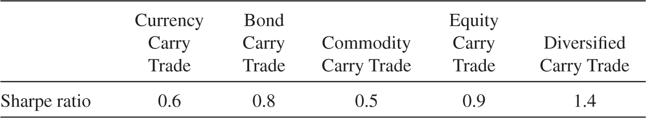
Source: Koijen, Moskowitz, Pedersen, and Vrugt (2012).
Macro traders pay tremendous attention to central banks. Why? Well, because that’s where the money is (to paraphrase Willie Sutton). Central banks control short-term interest rates, which has implications across all markets. For example, the interest rate determines the currency carry and bond prices. Therefore, macro investors monitor central banks, trying to predict their next move. Is the central bank about to raise interest rates or lower them? If the central bank is about to lower rates, how large will the rate cut be: 25 basis points (bps), 50 bps, or more? Will the central bank signal a hawkish or dovish stance that will change the market’s expectations about future rate changes? Will it implement unconventional monetary policies, such as lending facilities or quantitative easing (i.e., buying long-term bonds) or increase the strength of such programs (e.g., buying more bonds per month or “tapering” such a purchase program)?
To answer these questions, macro traders seek to understand each central bank’s objectives and policy constraints and to analyze the same economic data as the central bank. Central bank objectives differ across countries. In the United States, the Federal Reserve has a “dual mandate” of price stability and maximum employment. This dual mandate can be summarized by saying that the Fed sets the nominal interest rate Rf approximately according to the Taylor rule (Taylor 1993):
![]()
where the output gap is the “percentage deviation of real GDP from its target,” meaning whether output is above or below its potential. One can simply think of the output gap as unemployment, more specifically, whether unemployment is below its “natural” level arising from job search delays and other things.2
The Taylor rule reflects that the Fed would like to keep inflation at 2% and the output gap at zero. In that case, the Fed sets a nominal interest rate of 4%, corresponding to a real interest rate (Rf—inflation) of 2%. If inflation rises above 2%, then the Fed raises nominal interest rates more than 1-for-1 (called the “Taylor principle”). Specifically, if inflation rises to 3%, then the Fed increases the nominal rate to 5.5%. Hence, the real interest rate goes up to 2.5%, and this rise in the real rate is meant to cool the economy, bringing inflation back down toward its target. Similarly, a negative output gap, i.e., high unemployment, results in lower interest rates that stimulate the economy.
The Taylor rule is only an approximation of the actual behavior of the Fed, and several other parameter choices and extensions have been suggested, though none perfectly match the Fed’s actual choices. For instance, macro economists have noted that the Fed often acts with a certain amount of inertia, preferring to raise interest rates only gradually.
Other central banks, such as the European Central Bank (ECB), have a single objective of price stability, that is, to keep inflation relatively constant (often around 2%). Countries with a pegged exchange rate must also use their monetary policy to achieve the exchange-rate objective, raising interest rates when the currency is falling in value and lowering interest rates when it is rising. Increasingly, central banks also have a financial stability goal.
Global macro traders obsess about central bank actions for two reasons. First, and most importantly, central bank actions move asset prices, and it is rewarding to be positioned correctly for the next central bank action. Second, central banks are active in the money markets, bond markets, and currency markets, and since they are not trading to maximize profit, their actions sometimes give rise to trading opportunities.
So how do macro investors trade based on their views on monetary policy? The simplest way is to buy bonds or interest rate futures if they think the central bank is lowering rates, and go short if they think the central bank is raising rates. They might also speculate on the slope of the yield curve since a central bank rate hike raises short-term interest rates more than long-term interest rates, thus flattening the yield curve. Macro traders might also bet on future central bank actions using forward-interest-rate markets.
Understanding central bank actions is also useful for currency trading. When the interest rate goes up, the carry improvement may attract capital and lead to currency appreciation. Foreign exchange markets are affected more directly by central banks when they actively intervene, buying or selling currency. Predicting such interventions and their timing is difficult, but some general patterns may emerge. If central banks generally try to dampen exchange-rate swings, then exchange rates move only slowly toward their new fundamentals, creating trends in currency markets that macro traders can exploit as discussed below in section 11.4.
Example: The Greenspan Briefcase Indicator
Many macro traders were religiously following Alan Greenspan when he was the chairman of the Federal Reserve. Perhaps for this reason, he made intentionally ambiguous statements using language that was dubbed “Fedspeak.” (Chairman Bernanke, in contrast, believed that transparency is more helpful.) Traders monitored Greenspan’s every move, especially on the days when the Federal Open Market Committee (FOMC) would decide on the new interest rate target.
As he walked to work on such a day, traders would already have figured out (e.g., based on the Taylor rule or recent Fedspeak) whether interest rates were heading upward or downward, leaving open the question: Will the Fed change the interest rate or leave it unchanged? The answer lay inside Greenspan’s briefcase, invisible to traders. However, the thickness of the briefcase held the answer, or so the thinking went: A thick briefcase meant lots of argument, leading to a rate change. A thin briefcase meant keeping interest rates the same. Hence, Greenspan’s briefcase was carefully watched (e.g., on live TV) when he walked into the Federal Reserve on FOMC days. Supposedly, in later years, Greenspan had his briefcase transported into the Fed hidden in the trunk of a car on such days, leaving Greenspan to stroll to work, arms free.
11.3. TRADING ON ECONOMIC DEVELOPMENTS
The Holy Grail for global macro traders is to know where the economy is moving. In particular, they want to know whether economic growth will be strong or slow and whether inflation is picking up or calming down. The combination of growth and inflation determines the economic environment, as illustrated in table 11.2.
If growth is strong and inflation high, the economy is doing well but may be “overheating,” leading the central bank to increase interest rates. Hence, in such an environment, bond prices drop and macro investors anticipating this eventuality sell bonds short. While the yield curve may be steep in the early stages of an overheated economy, central bank actions are likely to flatten the curve over time as the policy interest rate is raised.
Stocks should do well in an overheated economy as growth fuels their profit and inflation does not affect their value (since their earnings will grow with inflation and thus keep their real value). Also, credit default swaps should fare well, while corporate bonds should see falling credit spreads, but prices will be dragged down by their interest-rate exposure.
TABLE 11.2. FOUR ECONOMIC ENVIRONMENTS DEPENDING ON GROWTH AND INFLATION
|
Strong Growth |
Slow Growth |
High inflation |
Overheated |
Stagflation |
Low inflation (or deflation) |
Goldilocks |
Lost decade |
In a “Goldilocks” economy, not-too-hot and not-too-cold, both stocks and bonds can do well. Volatility might be falling, lowering option prices, but we must be aware that the calm will not last forever.
Stagflation is a central bank’s nightmare because fighting the inflation with higher interest rates means further hurting the stagnating economy. Stocks suffer due to the poor growth prospects, and bonds suffer due to inflation. Commodities and Treasury inflation-protected securities (TIPS) may do well, at least in nominal terms, due to their inflation protection, and gold prices may also benefit from a flight to quality.
In a “lost decade” with low inflation and slow growth, bond yields are likely to fall, meaning that bond prices rise. For example, after the global financial crisis of 2008–2009, bond yields started falling and, while some investors repeatedly noted that yields could now only go up, bonds yields kept falling. Similarly, Japanese bond yields kept falling through the 1990s and, to a lesser extent, the 2000s.
Global macro hedge funds analyze the economic environment and make directional investments based on their analysis. Macro investors also consider relative-value trades, comparing different countries’ relative growth and inflation developments. Such traders bet on which asset classes in which countries will outperform and which will underperform as we discuss further in section 11.4. First, we need to explore what determines the state of the economy.
The state of the economy is determined by aggregate supply and demand, and we consider their respective underlying drivers. There are several competing models in modern macroeconomics, but I focus on a simple model that captures the ideas that many macro traders and policy makers have in mind when they think about economic questions.
What Drives Aggregate Supply?
Macro economists want to determine a country’s aggregate supply of output, i.e., the gross domestic product (GDP), often referred to with the symbol Y. This output is produced by the country’s labor (L) and capital (K). The labor L refers to the number of people who work. A country’s physical capital K refers to its machines, plants, natural resources, computers, trucks, and infrastructure that are put to use. The output supplied can be thought of as using production function F:
![]()
where TFP is the total factor productivity, which measures how good the technology is, how well educated and skillful the population is, and how efficiently capital and people are allocated to the most productive sectors.
In the long run, that is all there is to it: Output is what the country can produce with the people and machines that it has. Prices and wages adjust to ensure that supply equals demand, and long-run GDP simply depends on the labor, capital, and production technology. Hence, macro traders look at population growth, education, investment, and technological innovation to determine long-run growth.
Short-run economic fluctuations are more complex, however. In the short run, a central determinant of aggregate supply is the employment rate. The labor used in production L depends not only on the country’s overall available labor force but also on what fraction of the people actually work. Unemployment means fewer hands adding to the country’s output. Similarly, output depends on the utilization rate of capital, meaning whether machines are idle or running at full speed.
Short-run economic dynamics are therefore closely connected to unemployment, and unemployment is related to inflation. The “Phillips curve” states that, in the short run, inflation increases with employment (as well as with expectations about future inflation). Since the supply of output increases with employment, output supply is also positively related to inflation in the short run, and this relation is represented as the aggregate supply (AS) curve in figure 11.2.
So why might inflation be positively related to employment? This may be because nominal wages are “sticky” in the short term, meaning that it takes time to change people’s salary expectations and to renegotiate salaries. With sticky wages, higher-than-expected price inflation for output goods implies that firms earn higher profits and therefore hire more people. Said differently, if nominal wages stay relatively constant while output prices increase surprisingly, then real wages decline, and firms want to hire. Therefore, (unexpected) inflation tends to be positively related to employment and supply in the short term. (In the long term, expectations adjust to the level of inflation such that wages follow suit, implying that permanently higher inflation has no effect on supply, at best.)
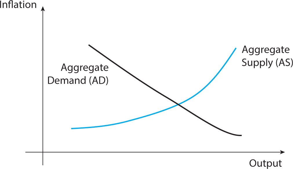
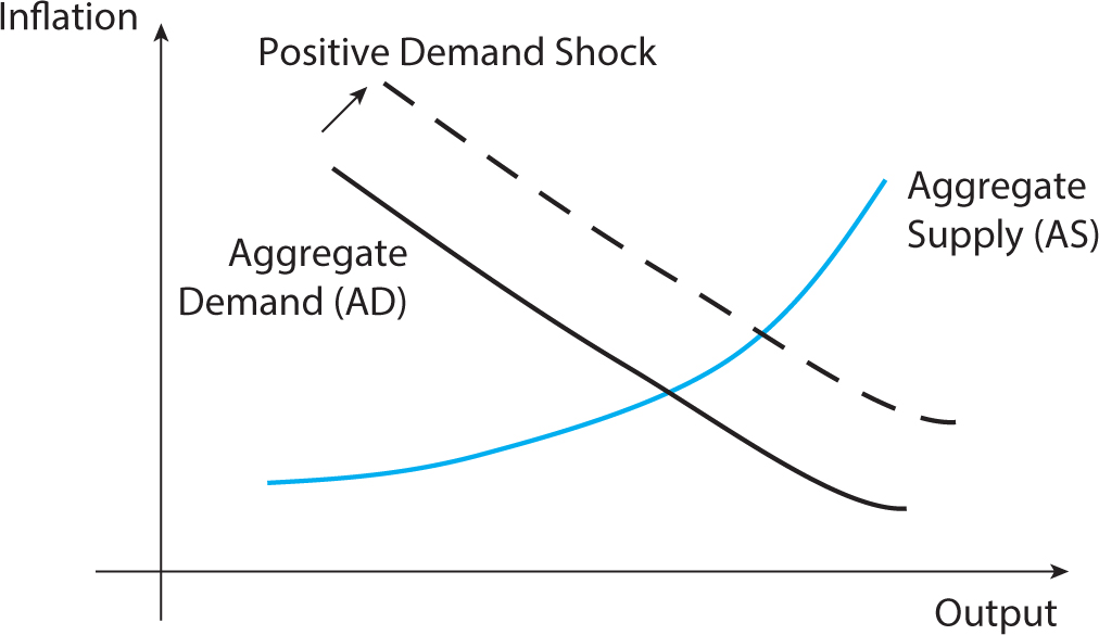
Figure 11.2. Short-run aggregate supply and demand curves.
In the short run, output depends on demand as well as supply. To link aggregate demand to inflation, modern economists first consider the behavior of central banks as discussed in section 11.2.3 Since central banks want to control inflation, higher inflation leads to higher real interest rates. This is seen from the Taylor rule in equation 11.1.
How then does the interest rate affect demand? To see this, note that the aggregate demand for output (Y) consists of demand from consumption (C), investment (I), government spending (G), exports (X), less imports, (M):
![]()
To figure out how demand depends on interest rates, consider first the determinants of private consumption, C. A lower interest rate increases private spending because it makes it cheaper to borrow (e.g., to take a car loan or credit card loan) and less attractive to save for the future. Private spending also depends on income and expectations about future income. Since income equals output Y, a multiplier effect can enhance the interest-rate sensitivity of consumption.
A lower interest rate also increases real investment I. This is because firms find it profitable to construct new plants and machines when they can be financed at a lower rate. Government spending, exports, and imports are relatively insensitive to interest rates, but they constitute possible demand shocks (e.g., due to changes in trade patterns as discussed later).
In conclusion, a lower interest rate raises aggregate demand (which is called the investment–saving curve or IS curve). Furthermore, recall that lower inflation leads to lower interest rates. Putting these two insights together explains why lower inflation leads to higher aggregate demand, as seen in the AD curve in figure 11.2.
Supply and Demand Shocks Determine Growth and Inflation
Short-run output and inflation are determined as the equilibrium point where aggregate supply meets demand in figure 11.2. Macro investors are not satisfied with understanding the current state of the economy, however; they want to know what happens next. They want to figure out whether economic growth will rise or slow down and whether inflation is about to pick up or quiet down. These changes are what move asset prices, and macro investors want to be positioned correctly for the next big move.
To figure out what happens next, macro economists must consider the shocks that are about to hit the economy and what effects they will have. One possibility is a positive demand shock, as illustrated in figure 11.3. Suppose, for example, that aggregate demand increases because of stronger consumer confidence or monetary easing (i.e., an interest rate below the level prescribed by the Taylor rule). As seen in figure 11.3, this increase raises both output and inflation, leading to rising stock prices and falling bond prices. Hence, if a macro investor anticipates rising aggregate demand—or anticipates that rising demand is more likely than reflected in current prices—then she might buy stocks and short-sell bonds.
TABLE 11.3. SUPPLY AND DEMAND SHOCKS GENERATE FOUR TYPES OF ECONOMIC ENVIRONMENTS
|
Strong Growth |
Slow Growth |
High inflation |
Positive demand shocks: Stronger consumer confidence Monetary easing Easier access to credit |
Negative supply shocks: Higher oil prices Depreciating capital Inefficient use of capital or trade |
Low inflation (or deflation) |
Positive supply shocks: Lower oil prices Better technology Labor market more global or more skilled |
Negative demand shocks: Weaker consumer confidence Money tightening Worse access to credit |
Alternatively, the demand shock can be negative, or the shock could come from the supply side. A supply shock (i.e., a change in the supply of goods for the same output prices) can be driven by a change in oil prices, technological innovation, or change in the labor market. These shocks correspond to up/down movements in the AS/AD curves, and the effects of these four types of shocks are illustrated in table 11.3.
Interestingly, we see that these demand and supply shocks are what generate the four economic environments from table 11.2. Demand shocks can generate an overheated economy or a lost decade, while supply shocks can generate Goldilocks or stagflation. Macro investors thus ponder the relative likelihood of supply and demand shocks when deciding on directional trades across asset classes.
The various types of supply and demand shocks occur over different time scales as some macro events drive the short-term dynamics (within a year), others affect the medium-term economic environment (1–5 years), and yet others determine the long-run growth (5+ years). The typical short-term demand shocks include changes in the consumer spending rate, changes in monetary policy, and changes in access to consumer credit (credit boom vs. banking crisis). Short-run supply shocks include changes in prices of natural resources, especially energy prices.
In the medium run, supply shocks can arise from changes in capital. Capital improvements are due to successful investments, including foreign direct investment (FDI). If a country fails to invest enough, its capital stock decreases as it depreciates and becomes obsolete. One driver of investment is how low the real interest rate is, which depends in part on the inflation risk premium
(i.e., stable inflation is best) and the rule of law. Also, supply shocks can arise from changes in labor-market frictions (sticky wages, search frictions, and rigid labor laws), product-market frictions (sticky prices and anticompetitive corporate measures), and capital-market frictions (market and funding illiquidity) leading to unemployment and lower capital utilization. For instance, a systemic banking crisis slows growth because the ability to finance projects is a driver of investment. In the long run, output depends on supply factors such as technological progress and population growth.
11.4. COUNTRY SELECTION AND OTHER GLOBAL MACRO TRADES
There are no limits to the kinds of trades that global macro hedge funds might consider. Here we consider some of the key trades based on relative-value country selection, momentum, trade flows, and political events.
Value and Momentum in Global Markets
As discussed in chapter 9, value and momentum strategies have worked well in individual equity markets over the past century. Such strategies are also pursued by global macro investors, though in very different macro markets. Macro momentum investing means buying markets that have outperformed, while shorting markets that have underperformed. For example, a global manager might buy equity indices in countries that are trending upward while shorting equity futures in countries that are lagging. The simplicity of this strategy makes it easy to generalize across markets.
Macro value investing means buying cheap markets while shorting expensive ones. For instance, a manager might compare the overall pricing of an equity market with where she thinks the fundamental value is. Of course, estimating fundamental value can be challenging, and there are many ways to approach it. Here is a simple way to think about value investing for several of the major global asset classes based on Asness, Moskowitz, and Pedersen (2013):
• Global equity index value trade: For equity indices, one can use the same techniques as in valuing individual equities. In other words, if you can value each of the stocks, just add up their value to get the fundamental value of the index and compare it to the overall price. One simple measure is the price-to-book ratio for the overall market (or other valuation ratios). Hence, one macro value trade is to buy “cheap” equity indices in countries with low price-to-book ratios while shorting equity indices with high ones.
• Currency value trade: For currencies, one measure of value can be derived using purchasing power parity (PPP). PPP says that goods should cost the same in all countries. Hence, if a burger (or a diversified basket of goods) costs more in euros than in US$, then the euro should fall in value going forward, resulting in a short-euro value bet.4 A simpler way to trade on currency value is to trade on long-term reversal, betting that currencies that have experienced large real appreciation (over five years, say) will eventually see a partial reversal of this move.
• Global bond value trade: A bond value trade is buying and selling 10-year bonds across countries globally. One measure of value is the real bond yield, that is, the yield minus the local inflation rate. Another simple measure is the current yield minus where the yield used to be for that country, focusing on long-run reversal. More sophisticated value measures would take into account each country’s risk of default (government debt, current account, and so on), the risk of future inflation, and global investment flows.
• Commodity value trade: Measuring the fundamental value of a commodity is difficult because it depends on a host of supply and demand factors. The simplest commodity value trade is to use long-run reversal (which also works in all the other asset classes), betting that commodities that have risen exceptionally in value will underperform those that have risen less.
Asness, Moskowitz, and Pedersen (2013) examine such global value and momentum trades in global equity, currency, bond, and commodity markets. Figure 11.4 plots the performance over time and reports the Sharpe ratios and correlations. The figure also shows the “combo” strategy of using both value and momentum signals together. As seen in the figure, value and momentum have worked in each of the asset classes. It is a testimony to the strength of these investment philosophies that they work both in individual equity markets and macro markets.
Value and momentum are highly negatively correlated. This makes sense because they are somewhat opposite trading ideas: One buys what looks cheap while the other buys what is trending upward (and may have become expensive as a result). However, value and momentum are not exact opposites since momentum looks at the short-run while value looks at the long run, and, as a result, both can make money on average. The strong negative correlation between value and momentum means that it is powerful to combine them as seen from the performance of the combo strategy. Many macro traders do just one or the other, however, as it is unintuitive to look for a cheap country that is trending upward—by definition you are missing the bottom.
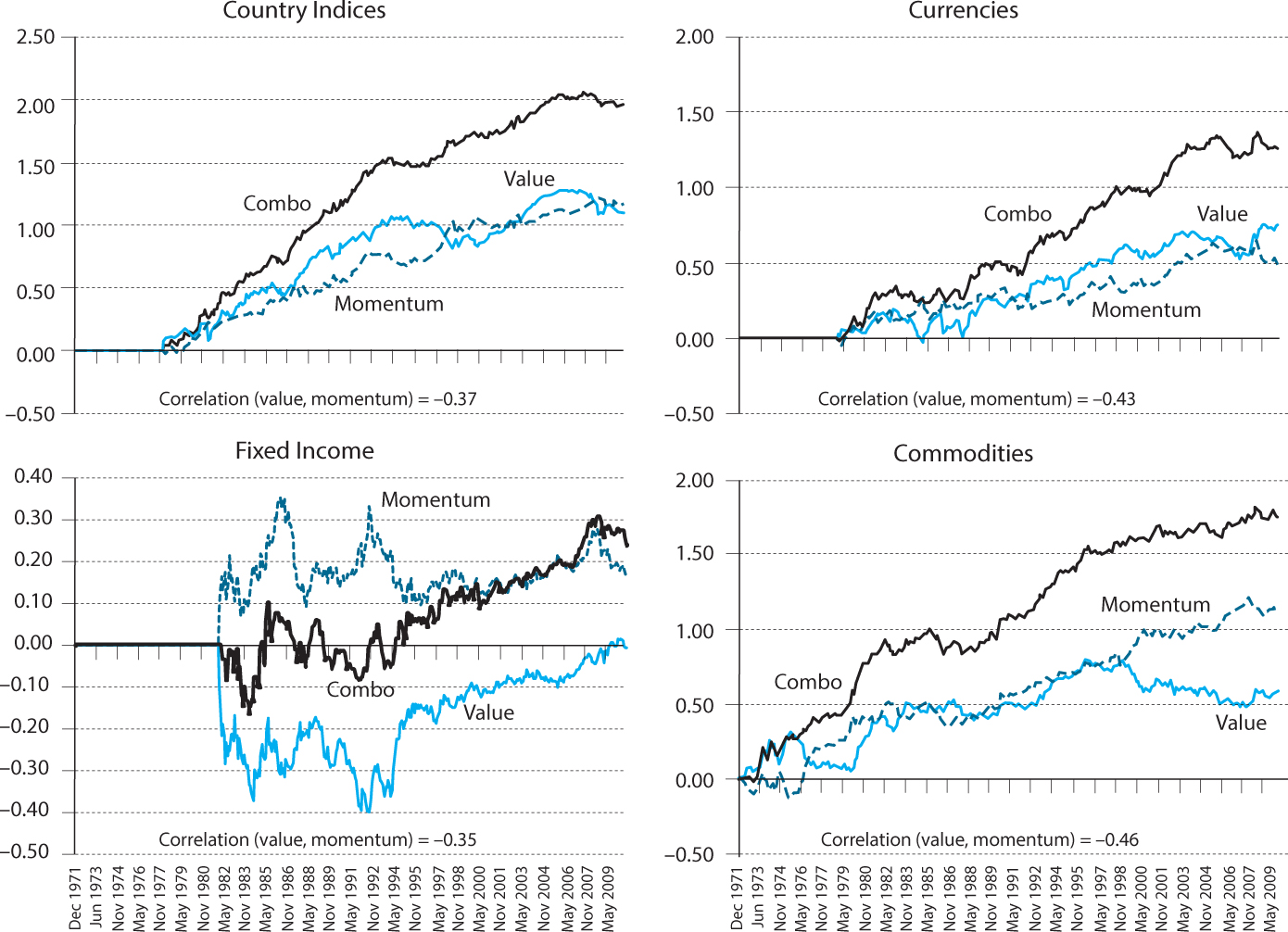
Figure 11.4. Value, momentum, and val-mom-combo strategies using equity country indices, currencies, fixed income, and commodity markets.
Source: Asness, Moskowitz, and Pedersen (2013).
Global Trade Flows and Terms of Trade
Global trade can be an important determinant of economic activity and exchange rates, especially for a small country. A country that exports more than it imports experiences buying pressure of its currency, which can lead to currency appreciation, especially if the buying pressure suddenly increases. Furthermore, the export sector fuels the domestic economy. Hence, some global macro investors try to predict changes in trade flows based on the new events that affect the relative supply and demand of exports and imports.
One important indicator is a country’s terms of trade, which measures the prices of the goods that a country exports relative to the prices of the goods that the country imports. For instance, suppose that South Africa exports diamonds and imports mining machines. If the price of diamonds rises relative to the price of machines, this is an improvement of South Africa’s terms of trade.
Macro traders may both track changes in terms of trade and try to predict their various implications. The increase in diamond prices will boost exports and create demand for the South African rand (ZAR), everything else being equal. While the diamond industry benefits, the exchange rate appreciation hurts other parts of the local economy, e.g., wine and textile exporters (a phenomenon called the “Dutch disease”).
The trade surplus is the major determinant of the current account surplus (which also includes interest income from foreign assets and foreign aid). A country’s current account surplus corresponds to its net increase in foreign assets, called a capital outflow. Capital flows and trade flows are therefore closely linked, and shocks to either can be important for exchange rates. For example, a country can experience strong capital inflows that push the exchange rate upward, leading to trade deficits.
Political Events and Regulatory Uncertainty
Changes in trade flows and terms of trade can influence exchange rates, but they can also work the other way. Sometimes countries try to influence their exchange rate to increase exports, and macro investors like to be attuned to such developments.
More generally, political events can be important for global macro developments. Countries may change their trade relations in various ways, opening or closing markets, imposing tariffs, imposing explicit or implicit trade barriers, and some countries face embargos due to strained intergovernmental relations.
The most extreme outcome of political events is a war, but more often macro traders look at more mundane new policies and legislation. They try to predict the consequences of the new legislation, e.g., which sectors will benefit and which sectors will be harmed.
11.5. THEMATIC GLOBAL MACRO
Some global macro traders focus on a few “big ideas” that they call “themes.” They believe that certain macro events will be important drivers of economic events in the future and then try to find various ways of profiting if the theme indeed plays out.
For instance, some global macro traders might believe that China’s growth will outpace what people expect. They might therefore buy Chinese stocks, buy commodities, especially those that China imports heavily, buy stocks in commodity-producing countries such as Australia, and possibly sell bonds if they believe that inflation will ensue. Another theme might be that China is instead in a bubble, leading the macro trader to take the opposite positions.
Yet another thematic global macro manager might believe that global warming is coming, buying carbon rights and windmill companies, or that oil production cannot keep up with demand, leading to rising energy prices.
Recently, an important theme has been systemic risk in the financial sector and sovereign credit risk. Some macro traders may focus on the likelihood that countries with large government debt will default or have inflation or that uncertainty and money growth will result in rising gold prices. Try to think of your own themes and create ways to trade on them.
11.6. GEORGE SOROS’S THEORY OF BOOM/BUST CYCLES AND REFLEXIVITY
George Soros is one of the most successful investors of all times. In addition to being a successful investor, he is a philanthropist, opinion maker, and philosopher. Soros has developed a theory of boom/bust cycles and reflexivity, as he describes in the following excerpt from a recent lecture.5
Let me state the two cardinal principles of my conceptual framework as it applies to the financial markets. First, market prices always distort the underlying fundamentals. The degree of distortion may range from the negligible to the significant. This is in direct contradiction to the efficient market hypothesis, which maintains that market prices accurately reflect all the available information. Second, instead of playing a purely passive role in reflecting an underlying reality, financial markets also have an active role: they can affect the so-called fundamentals they are supposed to reflect.
There are various pathways by which the mispricing of financial assets can affect the so-called fundamentals. The most widely traveled are those that involve the use of leverage—both debt and equity leveraging. The various feedback loops may give the impression that markets are often right, but the mechanism at work is very different from the one proposed by the prevailing paradigm. I claim that financial markets have ways of altering the fundamentals and that the resulting alterations may bring about a closer correspondence between market prices and the underlying fundamentals.
My two propositions focus attention on the reflexive feedback loops that characterize financial markets. I described the two kinds of feedback, negative and positive. Again, negative feedback is self-correcting, and positive feedback is self-reinforcing. Thus, negative feedback sets up a tendency toward equilibrium, but positive feedback produces dynamic disequilibrium. Positive feedback loops are more interesting because they can cause big moves, both in market prices and in the underlying fundamentals. A positive feedback process that runs its full course is initially self-reinforcing in one direction, but eventually it is liable to reach a climax or reversal point, after which it becomes self-reinforcing in the opposite direction. But positive feedback processes do not necessarily run their full course; they may be aborted at any time by negative feedback.
I have developed a theory about boom-bust processes, or bubbles, along these lines. Every bubble has two components: an underlying trend that prevails in reality and a misconception relating to that trend. A boom-bust process is set in motion when a trend and a misconception positively reinforce each other. The process is liable to be tested by negative feedback along the way. If the trend is strong enough to survive the test, both the trend and the misconception will be further reinforced. Eventually, market expectations become so far removed from reality that people are forced to recognize that a misconception is involved. A twilight period ensues during which doubts grow and more people lose faith, but the prevailing trend is sustained by inertia. As Chuck Prince, former head of Citigroup said: “As long as the music is playing, you’ve got to get up and dance. We’re still dancing.” Eventually a point is reached when the trend is reversed; it then becomes self-reinforcing in the opposite direction.
Let me go back to the example I used when I originally proposed my theory in 1987: the conglomerate boom of the late 1960s. The underlying trend is represented by earnings per share, the expectations relating to that trend by stock prices. Conglomerates improved their earnings per share by acquiring other companies. Inflated expectations allowed them to improve their earnings performance, but eventually reality could not keep up with expectations. After a twilight period the price trend was reversed. All the problems that had been swept under the carpet surfaced, and earnings collapsed. As the president of one of the conglomerates, Ogden Corporation, told me at the time: I have no audience to play to.
The chart below is a model of the conglomerate bubble. The charts of actual conglomerates like Ogden Corporation closely resemble this chart. Bubbles that conform to this pattern go through distinct stages: (1) inception; (2) a period of acceleration, (3) interrupted and reinforced by successful tests; (4) a twilight period; (5) and the reversal point or climax, (6) followed by acceleration on the downside (7) culminating in a financial crisis.
The length and strength of each stage is unpredictable, but there is an internal logic to the sequence of stages. So the sequence is predictable, but even that can be terminated by government intervention or some other form of negative feedback. In the case of the conglomerate boom, it was the defeat of Leasco Systems and Research Corporation in its attempt to acquire Manufacturer Hanover Trust Company that constituted the climax, or reversal point.
Typically, bubbles have an asymmetric shape. The boom is long and drawn out; slow to start, it accelerates gradually until it flattens out during the twilight period. The bust is short and steep because it is reinforced by the forced liquidation of unsound positions. Disillusionment turns into panic, reaching its climax in a financial crisis.

Figure 11.5. Soros’s theory of boom/bust cycles and reflexivity.
Source: Soros (2010).
The simplest case is a real estate boom. The trend that precipitates it is that credit becomes cheaper and more easily available; the misconception is that the value of the collateral is independent of the availability of credit. As a matter of fact, the relationship between the availability of credit and the value of the collateral is reflexive. When credit becomes cheaper and more easily available, activity picks up and real estate values rise. There are fewer defaults, credit performance improves, and lending standards are relaxed. So at the height of the boom, the amount of credit involved is at its maximum and a reversal precipitates forced liquidation, depressing real estate values.
Not all bubbles involve the extension of credit; some are based on equity leveraging. The best examples are the conglomerate boom of the late 1960s and the Internet bubble of the late 1990s. When Alan Greenspan spoke about irrational exuberance in 1996, he misrepresented bubbles. When I see a bubble forming I rush in to buy, adding fuel to the fire. That is not irrational. And that is why we need regulators to counteract the market when a bubble is threatening to grow too big; we cannot rely on market participants, however well informed and rational they are.
Bubbles are not the only form in which reflexivity manifests itself. They are just the most dramatic and the most directly opposed to the efficient market hypothesis; so they do deserve special attention. But reflexivity can take many other forms. In currency markets, for instance, the upside and downside are symmetrical so that there is no sign of an asymmetry between boom and bust. But there is no sign of equilibrium either. Freely floating exchange rates tend to move in large, multi-year waves.
The most important and most interesting reflexive interaction takes place between the financial authorities and financial markets. While bubbles only occur intermittently, the interplay between authorities and markets is an ongoing process. Misunderstandings by either side usually stay within reasonable bounds because market reactions provide useful feedback to the authorities, allowing them to correct their mistakes. But occasionally the mistakes prove to be self-validating, setting in motion vicious or virtuous circles. Such feedback loops resemble bubbles in the sense that they are initially self-reinforcing but eventually self-defeating. Indeed, the intervention of the authorities to deal with periodic financial crises played a crucial role in the development of a “superbubble” that burst in 2007–2008.
It will be useful to distinguish between near-equilibrium conditions, which are characterized by random fluctuations, and far-from-equilibrium situations, in which a bubble predominates. Near-equilibrium is characterized by humdrum, everyday events that are repetitive and lend themselves to statistical generalizations. Far-from-equilibrium conditions give rise to unique, historic events in which outcomes are generally uncertain but have the capacity to disrupt the statistical generalizations based on everyday events. The rules that can guide decisions in near equilibrium conditions do not apply in far-from-equilibrium situations. The recent financial crisis is a case in point.
Uncertainty finds expression in volatility. Increased volatility requires a reduction in risk exposure. This leads to what John Maynard Keynes called “increased liquidity preference.” This is an additional factor in the forced liquidation of positions that characterizes financial crises. When the crisis abates and the range of uncertainty is reduced, it leads to an almost automatic rebound in the stock market as the liquidity preference stops rising and eventually falls. That is another lesson I have learned recently.
11.7. INTERVIEW WITH GEORGE SOROS OF SOROS FUND MANAGEMENT
George Soros is the chairman of Soros Fund Management. One of the first and most successful hedge fund managers ever, he has been running his funds since 1973. He became known as “The Man Who Broke the Bank of England” when he made around $1 billion by short-selling the British pound during the 1992 U.K. currency crisis. Soros is also a prolific writer and has developed a theory of reflexivity. He was born in Budapest in 1930, survived the Nazi occupation of Hungary during World War II as well as the postwar imposition of Stalinism, fled to England, and graduated from the London School of Economics in 1952.
LHP: I have the impression that you have an incredible sense of the sentiment in the market, the prevailing biases, what regulators are considering, and what market participants are thinking. How did you get that insight?
GS: Over the years, I’ve developed a theory about markets. At one time, my theory was very different from the prevailing view. I focused on what I considered important in anticipating the future, rather than evaluating the present. I also noted interplay between politics and economics. So I considered actions by governments very important. At times, macro changes were important; at other times they were not. I looked at markets at various levels. There were times when I focused on the macro. At other times, I focused on a particular industry or company. It was an ever-changing game. I liked to say that I wasn’t the best at playing the market by any particular set of rules, but I was particularly attuned to changes in the rules. That’s really, I would say, what set me apart.
LHP: Can you describe how you were so attuned to those changes in the rules of the game?
GS: It was a constant process of learning. I talked to a lot of people. The markets were evolving. I look at markets not as timeless but changing with time. I view the markets as a historical process. My own involvement is an evolutionary process. My views are not timeless, but very time-bound.
LHP: Can you describe the evolution of your market involvement?
GS: The financial markets have changed dramatically since the end of the Second World War. Early on, they were very regulated. Currencies were regulated. Credit markets too. Take the banking system. I participated in the evolution of the banking system from the moment that it became interesting as an investment, which was in 1972. I wrote a paper called “The Case for Growth Banks.” At the time, bank shares were practically not traded. I felt this was about to change, and it did change in 1973, and there was a case for growth banks. Regarding emerging markets—in the early days they were not emerging, they didn’t exist! So, in the course of my history, I actually participated in the emergence of markets—let’s say, opening up the Swedish stock market. It was totally isolated and totally frozen.
LHP: Can you give an example of a macro trade you did and explain how you got the idea and how you convinced yourself that you had conviction on the trade?
GS: Well, the most convincing thing, I suppose, is my coming out of retirement, or semiretirement, to take an active role in anticipation of the financial crisis of 2008. I was largely withdrawn and out of date in my knowledge of the markets, but I believed there was a big macro development which was going to swamp other factors. I felt that I had to protect the estate that I had acquired over the years, and, you know, my money was being invested by others. It was a pretty large fund, where the positions tended to be on the long side so I opened a macro account where I hedged, basically, the positions of others and took positions that were net/net short.
LHP: How did you get conviction that this was going to be a major financial crisis before the market had recognized it?
GS: Well, because I had developed this boom/bust theory. Call it a theory of bubbles. I’ve written books about it. I published a book in ’98 when I said I thought that markets were about to collapse, The Crisis of Global Capitalism. The prediction turned out to be false; the markets didn’t collapse.
LHP: Well, it took a few more years.
GS: The authorities managed to contain the problem in 1998. You had Long-Term Capital Management, and it was a pretty serious situation, which was saved by Bill McDonough, the head of the Federal Reserve in New York. He put the players in one room and said, “You’ve got to do something!” And then they saved the day. So, we survived ’98. But by allowing what I call this super bubble to develop, it grew larger and finally exploded in 2008. In 2006, I published a book, The Age of Fallibility, where I had a very short section that previewed what was coming. In 2006, it was clear to me that it was coming. Even if it wasn’t clear when exactly it would come.
LHP: Right—you have this consistent record of understanding these boom/bust cycles. At a high level, I understand what you mean, but it might not be obvious to someone like me to know where we are in that cycle in any kind of situation.
GS: It wasn’t obvious to me, either. That’s the whole point, you see. A bubble is when a situation moves from near-equilibrium to far-from-equilibrium. So, you’ve got these two strange attractors where the whole thing is an interplay between perceptions and the actual state of affairs. You’ve got these two functions, the cognitive function and the participative function, and the interplay between them is reflexivity.
LHP: If I understand your investment process correctly, you’re comfortable positioning yourself both to profit from a boom, even as it pushes us farther away from the equilibrium state, and also positioning yourself to profit from the bust that happens as we move closer to the near-equilibrium state.
GS: Yes.
LHP: So, then how do you know when to switch from one to the other?
GS: I don’t know. My theory doesn’t tell me, because it’s actually unknowable, because it’s not predetermined. It’s determined by the actions and the attitudes of market participants and regulators. As a general rule, I would say that I’ve usually underestimated how far from equilibrium a situation can become. For instance, we lost a lot of money in 2000 when we thought that the IT bubble was collapsing, yet it had another revival.
LHP: But as an investor, you must decide when to position yourself long versus short. Are there some signs you look for to make that switch?
GS: Well, we’re looking. We know that it’s going to swing, but we don’t know when.
LHP: How did you think about what’s going to be the next move of Volcker or Greenspan or other policy makers?
GS: Well, it depends. Each—each occasion was different.
LHP: Was it putting yourself in their place?
GS: Well, yes. Naturally.
LHP: I would like to understand how you size your positions. In The Alchemy of Finance, you say: “I was willing to risk only gains, not my capital. This gave the fund its own momentum: picking up speed when the wind was behind us and trimming sails in stormy weather.” But, you have also emphasized taking very large positions when you have great conviction.
GS: Well, I take very large positions only when there is an asymmetry. For instance, betting against the European exchange rate mechanism was a low-risk bet. By taking a very large position, I wasn’t taking a large risk. That was also the case when John Paulson took a very large position against subprime mortgages because there was a disparity between the risk and the reward—he learned that from reading my book.
LHP: What are the typical situations with very favorable risk–reward ratios?
GS: There are many situations where there is a disparity between risk and reward. When you’ve got a fixed currency system, for instance. If a currency is fixed so it can only fluctuate within, say, a 2% band, then your downside risk in taking a short position is 2%, okay? However, if it breaks, then it can move much further. So, if you only have a 2% risk, you can take a large position.
LHP: And do you tend to reduce risk after losses and increase risk after gains?
GS: Well, generally speaking, you should not risk a significant part of your capital. Therefore, if you have a good run and you’re making a lot of profit, you can risk your profits more than you can risk your capital.
LHP: You’ve invested both in developed markets and emerging markets. Is there something different about investing in emerging markets?
GS: Yes, but then the emerging markets themselves change. So, let’s say Brazil was an emerging market, but now it’s got quite a lot of substance to it and is no longer behaving the way it used to.
Also, emerging markets in the early years emerged because people in America decided to invest. So foreign investors were dominating. And that, in itself, created a boom/bust situation, because the entrance of foreign investors created additional demand, which outweighed the domestic demand. So shares were revalued.
But foreign investors were just as liable to be attracted by this rapid appreciation as they were likely to be pushed to dump it when it went against them. So they were an external influence, and their entry and exit created a boom/bust sequence.
LHP: Finally, would you say that there is a specific experience that shaped you as an investor?
GS: The formative experience of my life was growing up in Nazi-occupied Hungary. That’s when I learned the difference between normal and far-from-equilibrium. In normal conditions, you play by normal rules, but in the German occupation, being a Jew, it was not normal. Because, you know, the Germans were killing normal citizens because they were Jewish; that’s not normal. So, you have to recognize that.
LHP: So do you also imply that it’s important as an investor to be able to face strong adversity and have the discipline to continue through tough periods?
GS: Right. All that. When the performance of a stock doesn’t correspond to your prediction, then something is wrong, and you need to identify what that is. And one of the things that can be wrong is your hypothesis. So you have to be constantly reexamining what it was that you believed in when you bought the stock.
___________________
1 In emerging markets, macro investors often look at each country’s real interest rate, that is, the nominal interest rate minus the inflation rate.
2 If one replaces the output gap with unemployment in the Taylor rule equation, then one must naturally also adjust the coefficients. To do this change, one can use the empirical relation (called Okun’s law) that the output gap is approximately equal to minus 2 times unemployment less the “natural rate of unemployment” (NAIRU). With a NAIRU of approximately 5% in the United States, this gives a Taylor rule of Rf = 4% + 1.5 × (inflation − 2%) − (unemployment − 5%). Note that empirically estimated Taylor rules differ significantly across time periods and countries. For instance, the constant term implies an average real rate of 2%, although the real rate has been significantly lower over a longer historical period.
3 This section is based on a version of an IS-MP model, that is, the combination of an investment-savings (IS) relation and the central bank’s monetary policy (MP) function. The MP function replaces the so-called LM curve (liquidity preference and money supply curve) in the traditional IS-LM model.
4 Especially for emerging markets, the PPP comparison should be adjusted for the Balassa–Samuelson effect that prices of non-tradable goods are systematically lower in poorer countries. For example, a haircut cannot easily be exported, and it is likely to remain cheaper in a poorer country even if iPad prices converge.
5 Soros (2010), “Financial Markets,” in The Soros Lectures, PublicAffairs, New York.