Chapter 1
Thinking About Chance

1. 1.1 Chapter Summary
2. 1.2 Glossary
3. 1.3 Equations
4. 1.4 Examples
5. 1.5 Exercises

Chapter Summary

In Chapter 1 we learn that probabilities are useful in thinking about events (things that occur or characteristics that exist) relative to observations (opportunities for things to occur or characteristics to exist). When thinking about probabilities, we use literary, graphic, or mathematic language. In literary language, a probability is the frequency of events relative to the number of observations. In graphic language, we use Venn diagrams to think about probabilities. In Venn diagrams, a circular area usually represents occurrences of the event and a rectangle represents the observations. Then, the probability of the event is reflected by the area of the circle relative to the area of the rectangle. Mathematically, probabilities are proportions, because the number of events is part of the number of observations.

Regardless of which language we use to think about probabilities, we notice that probabilities have certain properties. One of these is that a probability must have a value within the range of zero to one. A probability of zero tells us that the event never occurs. A probability of one tells us that the event always occurs. Probabilities between zero and one tell us that the event sometimes occurs.

In addition to thinking about single events, we can use probabilities to think about collections of events. The first collection of events considered in Chapter 1 includes the event and its complement. The complement of an event includes everything that could happen in an observation except the event. Events and their complements always have two characteristics. One is that they are always collectively exhaustive. Events are collectively exhaustive when at least one of the events must occur in every observation. Another characteristic of events and their complements is that they are mutually exclusive. Being mutually exclusive means that, at most, only one of the events can occur in a particular observation.

We can have collections of events other than just a particular event and its complement. Other collections of events might be collectively exhaustive and/or mutually exclusive. An event and its complement, however, are always collectively exhaustive and mutually exclusive.

With other collections of events, we can be interested in two types relationships of the events. These are the intersection and the union of those events. In an intersection of events, we are interested in those observations in which all of the events occur. In a union of events, we are interested in those observations in which at least one of the events occurs.

When we are interested in the intersection of events, we can use the multiplication rule to calculate the probability of the intersection. There are two versions of the multiplication rule. The simplified version involves multiplying the probabilities of each event together. This simplified version is appropriate if the events are statistically independent (from each other). That is, if the probability of each event is the same regardless of whether the other event(s) occur(s). The full version of the multiplication rule uses conditional probabilities.

Many of the probabilities we encounter in health research and practice are conditional probabilities. What distinguishes conditional probabilities from other probabilities is the fact that conditional probabilities address a subset of the observations, rather than all of the observations. That subset of observations is specified by the conditioning event(s). The event(s) addressed by the conditional probability is specified by the conditional event(s). If events are statistically independent, then the probability of the conditional event occurring is the same regardless of whether the conditioning event occurs.

When we are interested in the union of events, we use the addition rule to calculate the probability of the union. There are two versions of the addition rule. In the simplified version, the probabilities of the events in the union are added together. This simplified version of the addition rule can be used when the events are mutually exclusive. If the events are not mutually exclusive, the probabilities of their intersections need to be taken into account.

The conditional and conditioning events in conditional probabilities have very different functions. A conditional probability addresses the probability that the conditional event(s) will occur under the assumption that the conditioning event(s) has occurred. Often we find we are interested in the probability that the conditioning event will occur assuming the conditional event has occurred. One example of this situation is the relationship among the probabilities used in interpreting diagnostic tests. Tests are characterized by their sensitivities and specificities. The conditioning events in sensitivity and specificity are whether or not a person has the disease. To interpret the result of a diagnostic test, however, we want to consider the probability that a person has the disease. In other words, we want to change whether someone has the disease from being the conditioning event to be the conditional event. The way in which we exchange conditional and conditioning events is by using Bayes' theorem.

Glossary

1. Addition Rule – the method of calculating the union of two or more events. The simplified version involves adding the probabilities of the individual events together. The simplified version can be used if the events are mutually exclusive. The full version for the union of two events involves adding the probabilities of the events together and subtracting the probability of their intersection.
2. Bayes' Theorem – the mathematical description of the relationship between the probability of one event conditional on the occurrence of another event and the conditional probability of the second event conditional on the occurrence of the first event.
3. Chance – a process of producing events that has no apparent cause. For example, to say that chance affects whether or not a particular person in the population will be selected to be included in a sample, implies that we know of no characteristics of that person that make it more or less likely they will be selected. See Probability.
4. Collectively Exhaustive – a collection of events that includes all possible observations. For instance, being male or female is a collectively exhaustive set of genders.
5. Complement – (of an event) the occurrence of anything except the event. For example, if the event is being exposed to a particular carcinogen, the complement of that event is not being exposed to that carcinogen. An event and its complement are always mutually exclusive and collectively exhaustive.
6. Conditional Event – the particular event addressed by a conditional probability.
7. Conditional Probability – the chance that that a particular event will occur in an observation in which another event (or events) has occurred. For example, if we are interested in comparing the chance of getting a disease between persons who are either exposed or unexposed, a conditional probability of interest would be the probability of getting the disease given that a person is exposed.
8. Conditioning Event – the event that has occurred in an observation that influences the chance that the conditional event will occur in that same observation. For example, if we are interested in comparing the chance of getting a disease between persons who are either exposed or unexposed, the conditioning event would be exposure.
9. Event – something that happens or exists in an observation. Examples of events include being exposed, having a disease, being a woman, and being selected to be in a sample.
10. Frequency – how often something happens. For example, if there are 10 persons with a particular disease in a group of persons, the frequency of disease in the group is 10.
11. Independence – see Statistical Independence.
12. Intersection – observations that include all the events. For example, the intersection between being exposed and having a disease includes those persons who are both exposed and have the disease.
13. Multiplication Rule – the method of calculating the intersection of two or more events. The simplified version involves multiplying the probabilities of the individual events together. The simplified version can be used if the events are statistically independent. The full version for the intersection of two events involves multiplying the probability of one of the events by the probability of the other event, given that the first event occurs.
14. Mutually Exclusive – a collection of events in which only one event can occur in a given observation. For example, suppose that a disease has five stages and each person with the disease can only be in one of those stages. Then, the stages of that disease are mutually exclusive.
15. Observation – an opportunity for an event to occur. In health research, the most common observations are persons.
16. Probability – the chance that an event will occur. For example, the probability of someone developing a particular disease might be equal to 0.1. That implies that one-tenth of the observations will develop the disease. A probability is a proportion, so it can have values in the range of 0-1. See Chance and Proportion.
17. Proportion – a fraction in which the number in the numerator is also included in the denominator. A proportion has a discrete range of possible values ranging from zero to one.
18. Statistical Independence – a property of two (or more) events in which the probability of one event occurring is not affected by whether the other event (or events) has occurred. For example, if developing a disease and being exposed are statistically independent, the probability of developing the disease is the same regardless of whether a person is exposed.
19. Unconditional Probability – the probability of an event occurring regardless of whether another event has occurred. For example, the unconditional probability of developing a disease does not separate exposed from unexposed persons.
20. Union – observations which include one or more of a collection of events. For example, if we consider risk factors for breast cancer as a collection of events, the union of those risk factors includes persons who have at least one risk factor.
21. Venn Equations – a method of representing probabilities that combines graphic language (Venn diagram) and mathematic language (equation).
22. Venn Diagram – a graphic representation of the relationship between events and observations in which the area of a figure (usually a circle for events and a rectangle for observations) corresponds to the frequency of an event or observation. For example, a Venn diagram representing the occurrence of a disease would have a circle (representing persons with the disease) inside a rectangle (representing persons). The area of the circle relative to the area of the rectangle would be the same as the number of persons with the disease relative to the total number of persons.

Equations

$p(\overline{A})=1-p(A)$	the probability of the complement of event A as it relates to the probability of event A. (see Equation{1.2})
$\begin{array}{lll}p(A\text{and}B)\hfill & =\hfill & p(A)\cdot p(B|A)\hfill \\ \hfill & =\hfill & p(B)\cdot p(A|B)\hfill \end{array}$	the probability of the intersection of events A and B. Either of the events can be represented by an unconditional probability. Then, the other event is represented by a conditional probability. This is the multiplication rule. (see Equation {1.4})
$p(A|B)=p(A|\overline{B})=p(A)$	three probabilities that are equal to the same value if event A is statistically independent of event B. (see Equation {1.8})
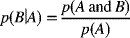$p(B|A)=\frac{p(A\text{and}B)}{p(A)}$	the probability of event B given that event A occurs. (see Equation {1.9})
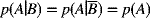
$p(A|B)=\frac{p(A\text{and}B)}{p(B)}$	the probability of event A given that event B occurs.
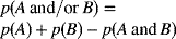$\begin{array}{l}p(A\text{and}/\text{or}B)=\hfill \\ p(A)+p(B)-p(A\text{and}B)\hfill \end{array}$	the probability of the union of events A and B. This is the addition rule. (see Equation {1.13})
$\begin{array}{l}p(B|A)=\hfill \\ \frac{p(B)\cdot p(A|B)}{\left[p(B)\cdot p(A|B)\right]+\left[p(\overline{B})\cdot p(A|\overline{B})\right]}\hfill \end{array}$	the relationship between the probability of event B occurring given that event A occurs and the probability of event A occurring given that event B occurs. This is Bayes' theorem. (see Equation {1.18})

Examples

Suppose 25 persons who ate a buffet lunch at a particular restaurant developed salmonella infections (a type of food poisoning). As epidemiologists, we are interested in finding out what food from the buffet was associated with becoming ill. To investigate this, we ask the 25 persons who became ill (the cases), and another 100 persons who ate at the buffet, but did not become ill (the controls), what they ate. Imagine we observe the following results for the items offered that are most likely to be the source of the infection:

Table 1.1 Frequencies of eating different foods for cases and for controls.

FOOD	CASES	CONTROLS
Potato salad	10	40
Chicken salad	5	20
Egg salad	2	8
Seafood salad	5	20
Cole slaw	4	16
Deviled eggs	8	32
Turkey	12	18
Dressing	12	24
Chicken	10	40

Eating a particular food is considered an event.

1.1. Are these events mutually exclusive?

To be mutually exclusive, the probability of one event occurring given that another event has occurred must be equal to zero. In this context, mutual exclusion would mean that a person could not eat both turkey and dressing, for example. This is illustrated in Figure 1.1.

Figure 1.1 Venn diagram illustrating mutual exclusion between eating turkey and eating dressing.

This is not likely to be true. Further, we can tell that at least some of the people ate more than one item. Among cases, the total number of items eaten is 68, but there are only 25 cases. Among the controls, the total number of items eaten is 218, but there are only 100 controls. The only explanation for those frequencies is that some people ate more than one item.

1.2. Are these events collectively exhaustive?

To be collectively exhaustive, all of the possible events must be listed. We are told that the listed items were “most likely to be the source of infection.” This implies that there were other items on the buffet that were unlikely to cause a salmonella infection. If there were other items on the buffet, then the listed foods are not collectively exhaustive.

To determine which foods might be the source of the infection, we want look at the associations between each type of food eaten and becoming ill. An association between events is the same as the events not being statistically independent.

1.3. To look for statistical independence, what type of probabilities are going to be of primary interest? Why?

Statistical independence is defined by the relationship between conditional probabilities. If two events are statistically independent, then the probability of one event is the same regardless of whether another event occurs. Here, statistical independence means the probability of eating any particular item is the same for cases as it is for controls.

Next, we will change the data in Table 1 so that they reflect probabilities of eating each of the foods for cases and for controls.

1.4. What will be the numerator of those probabilities?

The numerator will be the number of cases eating a particular food or the number of controls eating a particular food.

1.5. What will be the denominator of those probabilities?

The denominator will be the number of cases or the number of controls.

1.6. Put the results of these calculations in a table.

Table 1.2 Probabilities of cases and controls eating particular foods.

FOOD	CASES	CONTROLS
Potato salad	$\raisebox{1ex}{$10$}\!\left/ \!\raisebox{-1ex}{$25$}\right.=0.40$	$\raisebox{1ex}{$40$}\!\left/ \!\raisebox{-1ex}{$100$}\right.=0.40$
Chicken salad	$\raisebox{1ex}{$5$}\!\left/ \!\raisebox{-1ex}{$25$}\right.=0.20$	$\raisebox{1ex}{$20$}\!\left/ \!\raisebox{-1ex}{$100$}\right.=0.20$
Egg salad	$\raisebox{1ex}{$2$}\!\left/ \!\raisebox{-1ex}{$25$}\right.=0.08$	$\raisebox{1ex}{$8$}\!\left/ \!\raisebox{-1ex}{$100$}\right.=0.08$
Seafood salad	$\raisebox{1ex}{$5$}\!\left/ \!\raisebox{-1ex}{$25$}\right.=0.20$	$\raisebox{1ex}{$20$}\!\left/ \!\raisebox{-1ex}{$100$}\right.=0.20$
Cole slaw	$\raisebox{1ex}{$4$}\!\left/ \!\raisebox{-1ex}{$25$}\right.=0.16$	$\raisebox{1ex}{$16$}\!\left/ \!\raisebox{-1ex}{$100$}\right.=0.16$
Deviled eggs	$\raisebox{1ex}{$8$}\!\left/ \!\raisebox{-1ex}{$25$}\right.=0.32$	$\raisebox{1ex}{$32$}\!\left/ \!\raisebox{-1ex}{$100$}\right.=0.32$
Turkey	$\raisebox{1ex}{$12$}\!\left/ \!\raisebox{-1ex}{$25$}\right.=0.48$	$\raisebox{1ex}{$18$}\!\left/ \!\raisebox{-1ex}{$100$}\right.=0.18$
Dressing	$\raisebox{1ex}{$12$}\!\left/ \!\raisebox{-1ex}{$25$}\right.=0.48$	$\raisebox{1ex}{$24$}\!\left/ \!\raisebox{-1ex}{$100$}\right.=0.24$
Chicken	$\raisebox{1ex}{$10$}\!\left/ \!\raisebox{-1ex}{$25$}\right.=0.40$	$\raisebox{1ex}{$40$}\!\left/ \!\raisebox{-1ex}{$100$}\right.=0.40$

1.7. What kind of probabilities are those in Table 1.2?

They are conditional probabilities with case or control as the conditioning event and eating a particular food as the conditional event.

1.8. If there is an association between eating a particular type of food and becoming ill, what relationship would we expect to see between the pairs of probabilities in Table 1.2?

If there is association between eating a particular type of food and becoming ill, then the conditional probabilities for that item will be unequal. Equal conditional probabilities are a sign of statistical independence, which is the same as no association.

1.9. For which food(s) is there an association with becoming ill?

The conditional probabilities for turkey and dressing are equal to different values for cases compared to controls. Cases had a higher probability of eating either of those foods than did controls.

1.10. Now, suppose no one ate both chicken and turkey. What do we call the relationship between those two events?

When the probability of one event is equal to zero if another event occurs, we call the events mutually exclusive.

Suppose we are interested in the probability that someone ate either turkey or chicken.

1.11. In what type of relationship between those events are we interested?

When we are interested in the probability of one and/or more events occurring, we are interested in the union of those events.

1.12. What is the probability that a case ate either turkey or chicken if no one ate both?

We find the union of two or more events by using the addition rule. When the events are mutually exclusive, we can use the simplified version of the addition rule.

$$p(\text{turkey or chicken}|\text{case})=p(\text{turkey}|\text{case})+p(\text{chicken}|\text{case})=0.48+0.40=0.88$$

Therefore, 88% of the cases ate either turkey or chicken.

1.13. What is the probability that a control ate either turkey or chicken if no one ate both?

Again, we are interested in the union of eating turkey and/or chicken. Since no one ate both, we can use the simplified version of the addition rule.

$$p(\text{turkey or chicken}|\text{control})=p(\text{turkey}|\text{control})+p(\text{chicken}|\text{control})=0.18+0.40=0.58$$

Therefore, 58% of the controls ate either turkey or chicken.

Now, suppose we are interested in how many people ate both potato salad and dressing.

1.14. In what type of relationship between those events are we interested?

When we are interested in both (all) events occurring in the same observation, we are interested in the intersection of the events.

1.15. If the probability of eating potato salad given that someone ate dressing is equal to 0.2 for both cases and controls, what is the probability that a case ate both potato salad and dressing?

Here, we are asked to calculate the probability of the intersection of eating potato salad and eating dressing for cases. We are told the probability of eating potato salad given that a case ate dressing is equal to 0.2. We know the events are not statistically independent since the conditional probability of eating potato salad is equal to 0.2, but the unconditional probability of eating potato salad among cases is 0.4 (from Table 2). Thus, we need to use the full version of the multiplication rule to calculate the probability of the intersection.

$$\begin{array}{lll}p(\text{Potato Salad and Dressing})\hfill & =\hfill & p(\text{Dressing})\cdot p(\text{Potato Salad}|\text{Dressing})\hfill \\ \hfill & =\hfill & 0.48\cdot 0.2=0.096\hfill \end{array}$$

1.16. What is the probability that a control ate both potato salad and dressing?

In this example, we are asked to calculate the probability of the intersection of eating potato salad and dressing among controls. The only difference between this example and the previous example is that we are considering controls. The conditional probability is the same for cases and controls, but the unconditional probability of eating dressing is different.

$$\begin{array}{lll}p(\text{Potato Salad and Dressing})\hfill & =\hfill & p(\text{Dressing})\cdot p(\text{Potato Salad}|\text{Dressing})\hfill \\ \hfill & =\hfill & 0.24\cdot 0.2=0.048\hfill \end{array}$$

Exercises

1.1. In a particular high school, 40 of the 200 graduating seniors report they have had unprotected sexual intercourse and 100 of the 200 graduating seniors report they have tried smoking marijuana at least once during high school. Further, 30 of the 100 graduating seniors who report they have tried smoking marijuana have also had unprotected sexual intercourse. Based on that information, which of the following is the best description of the relationship between having unprotected sexual intercourse and smoking marijuana?

1. Having unprotected sexual intercourse and smoking marijuana are not statistically independent but they are mutually exclusive.
2. Having unprotected sexual intercourse and smoking marijuana are statistically independent but they are not mutually exclusive.
3. Having unprotected sexual intercourse and smoking marijuana are both statistically independent and mutually exclusive.
4. Having unprotected sexual intercourse and smoking marijuana are neither statistically independent nor mutually exclusive.
5. There is not enough information given here to determine statistical independence and mutual exclusion of having unprotected sexual intercourse and smoking marijuana.

1.2. Suppose 25% of the children in a certain elementary school developed nausea and vomiting following a holiday party. None of the children who drank the apple cider at that party became ill. Based on that information, which of the following is the best description of the relationship between becoming ill and drinking apple cider at the party?

1. Becoming ill and drinking cider are not statistically independent but they are mutually exclusive.
2. Becoming ill and drinking cider are statistically independent but they are not mutually exclusive.
3. Becoming ill and drinking cider are both statistically independent and mutually exclusive.
4. Becoming ill and drinking cider are neither statistically independent nor mutually exclusive.
5. There is not enough information given here to determine statistical independence and mutual exclusion of becoming ill and drinking cider.

1.3. In a particular population, 30% of the people smoke cigarettes and 10% of the people have chronic obstructive pulmonary disease (COPD). If having COPD is independent of smoking, what percent of the population would you expect to find who smoke and also have COPD?

1. 0%
2. 3%
3. 10%
4. 30%
5. 40%

1.4. In a particular population, 5% of the infants have a low birthweight (<2,500 g) and 60% of the mothers have at least 16 years of education. If having a mother with at least 16 years of education and having a low birthweight are statistically independent, which of the following is closest to the percentage of infants who have a mother with at least 16 years of education and who have a low birthweight?

1. 0%
2. 3%
3. 6%
4. 30%
5. 40%

1.5. Suppose in a population of 10,000 persons, 5,000 smoke cigarettes and 7,500 have a high fat diet. Further, suppose that among the 5,000 persons who smoke cigarettes there are 3,000 who are also among the 7,500 who have a high fat diet. Based that information, which of the following is closest to the percentage of persons in the population who smoke cigarettes and/or have a high fat diet?

1. 38%
2. 50%
3. 75%
4. 88%
5. 125%

1.6. In a particular population, 60% of infants receive only their mother's breast milk, 20% receive only commercial infant formula, and 20% receive both. What is the chance that a particular infant selected randomly would receive breast milk and/or formula?

1. 0%
2. 20%
3. 80%
4. 100%
5. 120%

1.7. Suppose we are interested in the efficacy of a new treatment for anemia. To investigate this treatment, we randomly assign 50 persons with anemia to receive the new treatment and 50 persons with anemia to receive the standard treatment. Among those 100 persons, suppose 60% are cured. If there is no association between treatment and the chance of being cured, what percentage of the persons who received the new treatment would we expect to be cured?

1. 0%
2. 30%
3. 36%
4. 50%
5. 60%

1.8. In a certain industry, 20% of the workers develop liver disease and 40% develop respiratory disease. If there is no association between developing liver disease and developing respiratory disease, what percentage of the workers who develop liver disease would we expect to develop respiratory disease?

1. 0%
2. 8%
3. 20%
4. 40%
5. 100%