Chapter 9
Bivariable Analysis of a Nominal Dependent Variable

1. 9.1 Chapter Summary
2. 9.2 Glossary
3. 9.3 Equations
4. 9.4 Examples
5. 9.5 Exercises

Chapter Summary

Many of the statistical procedures we have examined in this chapter for a nominal dependent variable and one independent variable are very similar to the procedures described in Chapter 7 for bivariable data sets containing a continuous dependent variable. An example is the test for trend which involves estimation of a straight line to describe probabilities as a function of a continuous independent variable.

Testing the omnibus null hypothesis in trend analysis for a nominal dependent variable and a continuous independent variable is similar to the F-test in regression analysis in that hypothesis testing in trend analysis involves examination of a ratio of two estimates of the variation of data represented by the dependent variable. In regression analysis, the F-ratio is calculated by dividing the explained variation (the regression mean square) by the unexplained variation (the residual mean square). In trend analysis, we divide the explained variation by the total variation. The reason for this difference between regression analysis and trend analysis is that the total variation of a nominal dependent variable is a function of the point estimates and, therefore, is not subject to separate effects of chance. The ratio in trend analysis has a distribution that is the square of the standard normal distribution. The square of the standard normal distribution is represented by the chi-square distribution with one degree of freedom.

Another parallel between bivariable data sets that contain a continuous dependent variable and those that contain a nominal dependent variable can be seen when the independent variable is nominal. In both cases, the nominal independent variable has the effect of dividing values of the dependent variable into two groups. Similar to comparing means of a continuous dependent variable between two groups, comparison of probabilities between two groups of nominal dependent variable values can be accomplished by examining the difference between those probabilities.

Means are always compared by examining their difference. Estimates of nominal dependent variable values (e.g., probabilities) can be compared by examining their difference or by examining their ratio. A ratio of nominal dependent variable estimates allows us to consider the relative, rather than absolute, distinction between two groups. Differences can be used to compare probabilities or rates. Probabilities and rates can also be compared as ratios.

Another ratio that can be used to compare values of a nominal dependent variable is the odds ratio. The odds ratio is equal to the odds of the event represented by the dependent variable in one group divided by the odds of that event in the other group. Odds are equal to the number of observations in which the event occurred divided by the number of observations in which the event did not occur.

The difference and ratios we have examined thus far assume that two nominal variables are measured for each individual and that only the values of those variables indicate any relationship among the individuals in a set of observations. In another type of dataset for a nominal dependent variable and a nominal independent variable, individuals are paired based on characteristic(s) thought to be associated with values of the dependent variable. In this paired sample, one member of the pair has one value of the nominal independent variable, and the other member of the pair has the other value of the independent variable.

Paired nominal data are arranged in a 2 × 2 table that is different from the type of 2 × 2 table used to organize unpaired nominal data. Ratios and differences between probabilities are calculated from a paired 2 × 2 table using different formulas from those used for an unpaired 2 × 2 table, but the point estimates are the same regardless of which formula is used. That is not true for odds ratios, which must be estimated using the formula for paired data if the data are paired.

Statistical hypothesis testing for nominal dependent and independent variables uses the same statistical procedures to test the most common null hypothesis about differences as is used to test the most common null hypothesis about ratios. Those null hypotheses are that the difference is equal to zero and that the ratio is equal to one. If one of those null hypotheses is true, then both are true, since they both imply that the nominal dependent variable estimates in the two groups are equal.

Thus, we need only one method of hypothesis testing for probabilities (and odds) and one test for rates. In this chapter, we encountered three alternative methods to test null hypotheses about probabilities. The reason for presenting three alternative methods is that all three are commonly found in health research literature. The first method involves conversion of the difference between probabilities to a standard normal deviate. The standard error for that difference is calculated using a weighted average of the point estimates of the probability of the event in the population.

Another method, known as the chi-square test, is based on the 2 × 2 table. In this approach, observed frequencies for the four combinations of dependent and independent variable values are compared to what we would expect if the probability of the event were the same for each of the two groups. Calculation of expected values is based on the simplified version of the multiplication rule of probability theory. Then, observed and expected frequencies are compared for each cell of the 2 × 2 table. Their sum is a chi-square value with one degree of freedom.

The results of those two methods of hypothesis testing are exactly the same with the chi-square value being the square of the standard normal deviate. The popularity of the chi-square test is due, in part, to its ability for expansion to consider more than one dependent and/or independent variable. The chi-square test uses redundant information since only one cell of a 2 × 2 table needs to be known to determine values in all four cells assuming the marginal frequencies are known.

The third procedure we examined for probabilities and odds uses only one cell of the 2 × 2 table. This procedure is a slightly different normal approximation, known as the Mantel-Haenszel test.

For statistical hypothesis testing on paired nominal data, we calculate a chi-square statistic using a special method known as McNemar's test.

To test the null hypothesis that the difference between rates is equal to zero or that the ratio of rates is equal to one, we use a method that is similar to the Mantel-Haenszel procedure.

Glossary

1. 2 × 2 Table – a tabular description of frequencies for a nominal dependent variable and a nominal independent variable. The table consists of two rows and two columns delineating four cells.
2. Cell Frequency – the number of observations that correspond to a particular cell in a 2 × 2 table.
3. Chi-Square – a test statistic often used for a nominal dependent variable and (at least) one independent variable.
4. Concordant Pair – a pair of matched subjects in which both members of the pair have the same outcome.
5. Contingency Table – an R × C table in which there are R rows and C columns. 2 × 2 tables are a special type of contingency table.
6. Continuity Correction – a correction for a small bias that occurs when representing a discrete distribution with a continuous distribution.
7. Discordant Pairs – a pair of matched subjects in which each member of the pair has a different outcome.
8. Dummy Variable – a variable that represents nominal data with numeric, yet qualitative, values. See Indicator Variable.
9. Fisher's Exact Test – an analysis of a 2 × 2 table using its actual sampling distribution, rather than an approximation. See hypergeometric distribution.
10. Hypergeometric Distribution – the actual sampling distribution for 2 × 2 tables.
11. Indicator Variable – a variable that represents nominal data with numeric values. See Dummy Variable.
12. Marginal Frequency – frequencies in a 2 × 2 table that are sums of rows or columns.
13. Mantel-Haenszel Test – a chi-square test used to analyze 2 × 2 tables.
14. McNemar's Test – a chi-square test for paired 2 × 2 tables.
15. Paired 2 × 2 Table – a 2 × 2 table that describes the outcomes of pairs, rather than individuals.
16. Paired Design – a study in which subjects are matched to similar subjects to form pairs.
17. Test for Trend – strictly speaking, this is an examination of a tendency of the dependent variable to change in a particular direction as the independent variable increases. Most often used to refer to a regression analysis with a nominal dependent variable and a continuous independent variable.

Equations

$\theta =\alpha +(\beta ·X)$	population's regression equation for a test for trend. (see Equation {9.1})
${\chi }^2=\frac{\sum n_i·({\hat{p}}_i-\overline{p}{)}^2}{\overline{p}·(1-\overline{p})}=\frac{\text{Regression Sum of Squares}}{\frac{\text{Total Sum of Squares}}{\text{Total Degrees of Freedom}}}$	chi-square used in the test of the omnibus null hypothesis in a test for trend. (see Equation {9.4})
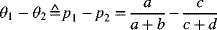${\theta }_1-{\theta }_2\stackrel{\wedge}{=}{p}_1-p_2=\frac{a}{a+b}-\frac{c}{c+d}$	probability difference. (see Equation {9.5})
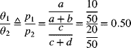
$\frac{{\theta }_1}{{\theta }_2}\stackrel{\wedge}{=}\frac{p_1}{p_2}=\frac{\frac{a}{a+b}}{\frac{c}{c+d}}$	probability ratio. (see Equation {9.6})
$OR\stackrel{\wedge}{=}\hat{O}R=\frac{\text{Odds of event in Group}1}{\text{Odds of event in Group}2}=\frac{\frac{a}{b}}{\frac{c}{d}}=\frac{a·d}{b·c}$	odds ratio. (see Equation {9.8})
${\chi }^2=\frac{{\left(a-E(a)\right)}^2}{E(a)}+\mathrm{.}..+\frac{{\left(d-E(d)\right)}^2}{E(d)}$	chi-square for a 2 × 2 table. (see Equation {9.17})
${\chi }^2=\frac{{\left(|a-E(a)|-\raisebox{1ex}{$1$}\!\left/ \!\raisebox{-1ex}{$/2$}\right.\right)}^2}{E(a)}+\mathrm{.}..+\frac{{\left(|d-E(d)|-\raisebox{1ex}{$1$}\!\left/ \!\raisebox{-1ex}{$/2$}\right.\right)}^2}{E(d)}$	chi-square for a 2 × 2 table with continuity correction. (see Equation {9.20})
$z=\frac{(p_1-p_2)-({\theta }_1-{\theta }_2)}{\sqrt{\frac{\overline{\theta }·(1-\overline{\theta })}{n_1}+\frac{\overline{\theta }·(1-\overline{\theta })}{n_2}}}$	standard normal test for a 2 × 2 table. (see Equation {9.18})
${\chi }^2=\frac{{(a-E(a))}^2}{\frac{(a+b)+(c+d)+(a+c)+(b+d)}{n^2·(n-1)}}$	Mantel-Haenszel chi-square for a 2 × 2 table. (see Equation {9.19})
$OR\stackrel{\wedge}{=}\hat{O}R=\frac{C}{B}$	odds ratio from paired 2 × 2 table. (see Equation {9.21})
${\chi }^2=\frac{{(C-B)}^2}{C+B}$	McNemar's chi-square for a paired 2 × 2 table. (see Equation {9.22})
$ID\stackrel{\wedge}{=}\hat{I}D=\frac{a}{P{T}_1}-\frac{b}{P{T}_2}$	incidence difference. (see Equation {9.23})
$IR\stackrel{\wedge}{=}\widehat{IR}=\frac{\frac{a}{P{T}_1}}{\frac{b}{P{T}_2}}$	incidence ratio. (see Equation {9.24})
${\chi }^2=\frac{{\left(a-\frac{(a+b)·P{T}_1}{P{T}_1+P{T}_2}\right)}^2}{\frac{(a+b)·P{T}_1·P{T}_2}{{(P{T}_1+P{T}_2)}^2}}$	chi-square to compare two incidences. (see Equation {9.25})

Examples

Suppose we are interested in the dose-response relationship for a medication for control of seizures and we observe the results in Table 9.1.

Table 9.1 Doses of a drug intended to control seizures.

Dose (mg)	n	Seizure
5	10	6
10	10	4
15	10	5
20	10	3
25	10	2

9.1. Have Excel make a scatter plot of these data.

9.2. Test the null hypothesis that occurrence of seizures is not related to dose. Allow a 5% chance of making a type I error.

$${\chi }^2=\frac{\text{Regression Sum of Squares}}{\frac{\text{Total Sum of Squares}}{\text{Total Degrees of Freedom}}}=\frac{0.81}{\frac{12}{49}}=3.3075$$

The critical value is from Table B.7. For α = 0.05 and one degree of freedom, the critical value is 3.841. Since the calculated value (3.3075) is less than the critical value (3.841), we fail to reject the null hypothesis.

Now, let us suppose we want to compare the efficacy of a new medication for control of seizures to the standard treatment. To do this, we randomly assign 100 persons to either the new medication or the standard treatment (i.e., 50 to each). Among the persons who were assigned to the new medication, 10 of them had at least one seizure during a two-week period of follow-up. By comparison, 20 of the persons assigned to the standard treatment had at least one seizure during that same period of follow-up.

9.3. Use that information to organize observations in a 2 × 2 table.

Table 9.2 2 × 2 table for two treatments intended to control seizures.

		Seizure
		Yes	No
Treatment	New	10	40	50
	Standard	20	30	50
		30	70	100

9.4. From that 2 × 2 table, calculate the two-week risks of seizure for the two treatment groups.

$$\begin{array}{lll}\text{Ris}{\mathrm{k}}_{\text{New}}\hfill & =\hfill & \frac{a}{a+b}=\frac{10}{50}=0.20\hfill \\ \text{Ris}{\mathrm{k}}_{\text{Stnd}}\hfill & =\hfill & \frac{c}{c+d}=\frac{20}{50}=0.40\hfill \end{array}$$

9.5. Calculate and interpret the risk ratio, risk difference, and odds ratio for the seizure data.

$$\frac{{\theta }_1}{{\theta }_2}\stackrel{\wedge}{=}\frac{p_1}{p_2}=\frac{\frac{a}{a+b}}{\frac{c}{c+d}}=\frac{\frac{10}{50}}{\frac{20}{50}}=0.50$$

The risk ratio tells us that persons taking the new medication have half the risk of seizures than do persons taking the standard treatment. The inverse of this ratio (1/0.5 = 2) tells us that persons taking the standard treatment have twice the risk of seizures than do persons taking the new medication.

$${\theta }_1-{\theta }_2\stackrel{\wedge}{=}{p}_1-p_2=\frac{a}{a+b}-\frac{c}{c+d}=\frac{10}{50}-\frac{20}{50}=-0.20$$

The risk difference tells us that the risk of seizures is reduced by 0.2 (20%) among persons taking the new medication.

$$OR\stackrel{\wedge}{=}\hat{O}R=\frac{a·d}{b·c}=\frac{10·30}{40·20}=0.375$$

The odds ratio tells us that the odds of having a seizure is 0.375 (37.5%) less among persons taking the new medication compared to persons taking the standard treatment. The inverse of this ratio (1/0.375 = 2.67) tells us that persons taking the standard treatment have two and two-thirds the odds of seizures than do persons taking the new medication.

9.6. Use the “2 × 2 Table Analyzer” BAHR program to analyze this 2 × 2 table. How do the results compare with your calculations?

When we use Excel to analyze these data, we get the following results:

These results are identical to those we got when we calculated these values by hand.

9.7. What are different ways to express the null hypothesis for a 2 × 2 table that directly address the risk ratio, risk difference, and odds ratio?

The usual null hypotheses we test from 2 × 2 table data are:

$$H_0:\frac{{\theta }_1}{{\theta }_2}=1H_0:{\theta }_1-{\theta }_2=0H_0:OR=1$$

All of these null hypotheses are true together or false together.

9.8. Use the Excel output to test the null hypothesis that the risks of seizure are the same in the two treatment groups.

In the output shown above, the P-values (to the far right) are less than 0.05. We do not need that information to answer the question, however. We could look at the confidence intervals and notice that the interval for the probability difference does not include zero and that the intervals for the probability ratio and odds ratio do not include one. All of that information means we can reject the null hypotheses.

One thing we do not want to do is to see if the confidence intervals for the two probabilities overlap. These are univariable confidence intervals. Two univariable confidence intervals are not a substitute for a bivariable hypothesis test!

Now, let us change the underlying frequency of seizures in both treatment groups by making it half of what is was. That would reduce the number of seizures in the group receiving the new medication from 10 to 5 and the number of seizures in the group receiving the standard treatment from 20 to 10.

9.9. Organize these data in a 2 × 2 table

Table 9.3 2 × 2 table for two treatments intended to control seizures with half the underlying frequency of seizures than Table 9.2.

		Seizure
		Yes	No
Treatment	New	5	45	50
	Standard	10	40	50
		15	85	100

9.10. Use the information in this new 2 × 2 table to calculate the two-week risks of seizure for the two treatment groups.

$$\begin{array}{c}\hfill p(\text{SEIZURE|NEW})=\frac{\text{Number of Persons on New Treatment with Seizure}}{\text{Total Number on New Treatment}}=\frac{5}{50}=0.1\hfill \\ \hfill p(\text{SEIZURE|STANDARD})=\frac{\text{Number of Persons on Standard Treatment with Seizure}}{\text{Total Number on Standard Treatment}}=\frac{10}{50}=0.2\hfill \end{array}$$

Both risks are half of what they were in the previous 2 × 2 table.

9.11. Calculate the risk ratio, risk difference, and odds ratio for these new data and compare them to the previous estimates.

$$RR=\frac{p(\text{SEIZURE}|\text{NEW})}{p(\text{SEIZURE}|\text{STANDARD})}=\frac{0.1}{0.2}=0.5$$

The risk ratio is not affected by the reduction of the underlying frequency of seizures.

$$RD=p(\text{SEIZURE}|\text{NEW})-p(\text{SEIZURE}|\text{STANDARD})=0.1-0.2=-0.1$$

The risk difference is half what it was when it was based on the original frequency of seizures. Thus, the risk difference reflects the underlying frequency of the event.

$$OR=\frac{ad}{bc}=\frac{5\text{√}40}{10\text{√}45}=0.44$$

The odds ratio has increased. As the underlying frequency of disease decreases, the odds ratio gets closer in value to the risk ratio.

Another way we could have designed this study would have been to give both treatments to each person at different times. This would be a paired study.

9.12. Suppose the study in Example 9.3 were done as a paired study. Further suppose eight persons had seizures on both treatments. Arrange those results in a paired 2 × 2 table.

The first step is to use the cell frequencies in the unpaired table as the marginal frequencies in the paired table. Next, put 8 in the upper left-hand cell. Finally, solve for the other cell frequencies by subtraction.

Table 9.4 Paired 2 × 2 table for two treatments intended to reduce the frequency of seizures.

		Standard
		SZ+	SZ−
New	SZ+	8	2	10
	SZ−	12	28	40
		20	30	50

9.13. Calculate the risk ratio, risk difference, and odds ratio for these new data and compare them to the previous estimates.

The risk ratio and risk difference in the paired table are the same as those estimates in the unpaired table. We can calculate them directly from the paired table by using the marginal frequencies.

$$\begin{array}{c}\hfill RR=\frac{p(\text{SEIZURE}|\text{NEW})}{p(\text{SEIZURE}|\text{STANDARD})}=\frac{\frac{10}{10+40}}{\frac{20}{20+30}}=0.5\hfill \\ \hfill RD=p(\text{SEIZURE}|\text{NEW})-p(\text{SEIZURE}|\text{STANDARD})=\frac{10}{10+40}-\frac{20}{20+30}=-0.2\hfill \end{array}$$

The odds ratio, on the other hand, is different when we have a paired study. It is calculated as:

$$OR=\frac{b}{c}=\frac{2}{12}=0.17$$

9.14. Test the null hypothesis that the risk of seizure is equal to the same value for both treatments, versus the alternative that they are not equal. If we allow a 5% chance of making a type I error, what should we conclude?

$${\chi }^2=\frac{{(b-c)}^2}{b+c}=\frac{{(12-2)}^2}{12+2}=7.143$$

From Table B.7, we find that the chi-square value that corresponds to 0.05 and one degree of freedom is equal to 3.841. Since the calculated chi-square is larger than the value from the table, we reject the null hypothesis and, through the process of elimination, accept the alternative hypothesis.

9.15. Use the “2 × 2 Table Analyzer” BAHR program to analyze these data. How do the results compare to what we have calculated by hand?

These are the same results we obtained by manual calculation.

Exercises

9.1. Suppose we are interested in the number of immunizations necessary to provide protection against hepatitis B infections. To investigate this, we identify a group of persons in a population in which hepatitis B is endemic who had 0, 1, 2, 3, 4, or 5 immunizations and follow them for a period of 10 years. Imagine we observe the data in the Excel file EXR9_1. These data use an indicator of hepatitis B as the dependent variable and the number of immunizations as the independent variable. From that information, estimate the 10-year risk of hepatitis B for a person who had 3 immunizations. Which of the following is closest to that estimate?

1. 0.09
2. 0.12
3. 0.15
4. 0.19
5. 0.24

9.2. In the Framingham Heart Study, 4,658 persons had their body mass index (BMI) calculated and were followed for 32 years to determine how many persons would develop heart disease (HD). Those data are in the Excel file EXR9_2. From those observations, estimate the probability that a person with a BMI of 30 would develop HD during a 32 year period. Which of the following is closest to that estimate?

1. 0.14
2. 0.21
3. 0.29
4. 0.33
5. 0.39

9.3. Suppose we are interested in the number of immunizations necessary to provide protection against hepatitis B infections. To investigate this, we identify a group of persons in a population in which hepatitis B is endemic who had 0, 1, 2, 3, 4, or 5 immunizations and follow them for a period of 10 years. Imagine we observe the data in the Excel file EXR9_1. These data use an indicator of hepatitis B as the dependent variable and the number of immunizations as the independent variable. From that information, test the null hypothesis that the number of immunizations does not help estimate risk versus the alternative hypothesis that it does help. If you allow a 5% chance of making a type I error, which of the following is the best conclusion to draw?

1. Reject both null and alternative hypotheses
2. Accept both null and alternative hypotheses
3. Reject the null hypothesis and accept the alternative hypothesis
4. Accept the null hypothesis and reject the alternative hypothesis
5. It is best not to draw a conclusion about the null and alternative hypotheses from these data

9.4. In the Framingham Heart Study, 4,658 persons had their body mass index (BMI) calculated and were followed for 32 years to determine how many persons would develop heart disease (HD). Those data are in the Excel file EXR9_2. From those observations, test the null hypothesis that knowing BMI does not help estimate the probability of HD versus the alternative that it does help. If you allow a 5% chance of making a type I error, which of the following is the best conclusion to draw?

1. Reject both null and alternative hypotheses
2. Accept both null and alternative hypotheses
3. Reject the null hypothesis and accept the alternative hypothesis
4. Accept the null hypothesis and reject the alternative hypothesis
5. It is best not to draw a conclusion about the null and alternative hypotheses from these data

9.5. Suppose we are interested in the number of immunizations necessary to provide protection against hepatitis B infections. To investigate this, we identify a group of persons in a population in which hepatitis B is endemic who had 0, 1, 2, 3, 4, or 5 immunizations and follow them for a period of 10 years. Imagine we observe the data in the Excel file EXR9_1. These data use an indicator of hepatitis B as the dependent variable and the number of immunizations as the independent variable. From that information, determine the 10-year risk of hepatitis B for persons who had no immunizations. Which of the following is closest to that risk?

1. 0.119
2. 0.146
3. 0.161
4. 0.261
5. 0.322

9.6. Suppose that we were to conduct a cohort study in which we identified 31 patients who had been diagnosed as having systemic hypertension and another group of 30 patients who had not been diagnosed with hypertension. We followed each of the groups to determine how many developed diabetes. At the end of the follow-up period, there were 25 persons who developed diabetes, 7 of whom did not have hypertension. From that information, which of the following is closest to the estimate of the risk of diabetes among exposed persons?

1. 0.25
2. 0.34
3. 0.42
4. 0.58
5. 0.66

9.7. Suppose that we were to conduct a cohort study in which we identified 31 patients who had been diagnosed as having systemic hypertension and another group of 30 patients who had not been diagnosed with hypertension. We followed each of the groups to determine how many developed diabetes. At the end of the follow-up period, there were 25 persons who developed diabetes, 7 of whom did not have hypertension. From that information, which of the following is closest to the estimate of the risk ratio comparing the risk of diabetes among exposed persons and among unexposed persons?

1. 0.52
2. 0.61
3. 1.05
4. 2.49
5. 5.14

9.8. Suppose we are interested in the number of immunizations necessary to provide protection against hepatitis B infections. To investigate this, we identify a group of persons in a population in which hepatitis B is endemic who had 0, 1, 2, 3, 4, or 5 immunizations and follow them for a period of 10 years. Imagine we observe the data in the Excel file EXR9_1. From these data, estimate the 10-year risk ratio comparing persons who received no immunization to persons who received at least one immunization. Which of the following is closest to that risk ratio?

1. 0.224
2. 0.581
3. 1.08
4. 1.65
5. 1.80

9.9. Suppose that we were to conduct a cohort study in which we identified 31 patients who had been diagnosed as having systemic hypertension and another group of 30 patients who had not been diagnosed with hypertension. We followed each of the groups to determine how many developed diabetes. At the end of the follow-up period, there were 25 persons who developed diabetes, 7 of whom did not have hypertension. From that information, test the null hypothesis that the risk ratio is equal to one in the population versus the alternative hypothesis that it is not equal to one. If you allow a 5% chance of making a type I error, which of the following is the best conclusion to draw?

1. Reject both null and alternative hypotheses
2. Accept both null and alternative hypotheses
3. Reject the null hypothesis and accept the alternative hypothesis
4. Accept the null hypothesis and reject the alternative hypothesis
5. It is best not to draw a conclusion about the null and alternative hypotheses from these data

9.10. Suppose we are interested in the number of immunizations necessary to provide protection against hepatitis B infections. To investigate this, we identify a group of persons in a population in which hepatitis B is endemic who had 0, 1, 2, 3, 4, or 5 immunizations and follow them for a period of 10 years. Imagine we observe the data in the Excel file EXR9_1. From these data, test the null hypothesis that the risk ratio is equal to one in the population versus the alternative hypothesis that it is not equal to one. If you allow a 5% chance of making a type I error, which of the following is the best conclusion to draw?

1. Reject both null and alternative hypotheses
2. Accept both null and alternative hypotheses
3. Reject the null hypothesis and accept the alternative hypothesis
4. Accept the null hypothesis and reject the alternative hypothesis
5. It is best not to draw a conclusion about the null and alternative hypotheses from these data