Chapter 10
Multivariable Analysis of a Continuous Dependent Variable

10.1 Chapter Summary
10.2 Glossary
10.3 Equations
10.4 Examples
10.5 Exercises

Chapter Summary

When we have a continuous dependent variable and more than one continuous independent variable, we can perform statistical procedures that are extensions of correlation analysis and regression analysis discussed in Chapter 7 for a single independent variable. For more than one independent variable the procedures are called multiple correlation analysis and multiple regression analysis. Both of those procedures examine a linear combination of the independent variables multiplied by their corresponding regression coefficients (slopes).

In analysis of multivariable data sets, we can think about the relationship of the dependent variable to each of the independent variables or about its relationship to the entire collection of independent variables. In multiple regression analysis, both are considered. In multiple correlation analysis, however, only the association between the dependent variable and the entire collection of independent variables is considered.

To interpret the multiple correlation coefficient (or, more appropriately, its square, the coefficient of multiple determination) as an estimate of the strength of association in the population from which the sample was drawn, all the independent variables must be from a naturalistic sample. That is to say, their distributions in the sample must be the result of random selection from their distributions in the population.

In multiple regression analysis, we can examine the relationship between the dependent variable and the entire collection of independent variables. The way we do this is by testing the omnibus null hypothesis.

We can also examine each individual independent variable in multiple regression analysis. The relationship between the dependent variable and an individual independent variable in multiple regression analysis, however, is not necessarily the same as the relationship between those variables in bivariable regression analysis (i.e., when we have only one independent variable). The difference is that, in multiple regression analysis, we examine the relationship between an independent variable and the variability in data represented by the dependent variable that is not associated with the other independent variables.

If two or more independent variables share information (i.e., if they are correlated) and, in addition, that shared information is the same as the information they use to estimate values of the dependent variable, we say we have collinearity (for two independent variables) or multicollinearity (for more than two independent variables). Multicollinearity (or collinearity) can make estimation and hypothesis testing for individual regression coefficients difficult. On the other hand, it makes it possible to take into account the confounding effects of one or more independent variables, while examining the relationship between another independent variable and the dependent variable. Multicollinearity is a feature, not only of multiple regression analysis, but of all multivariable procedures.

When we have more than one nominal independent variable, we are able to specify more than two groups of dependent variable values. The means of the dependent variable values for those groups are compared using analysis of variance (ANOVA) procedures. Analysis of variance involves estimating three sources of variation of data represented by the dependent variable. The variation of the dependent variable without regard to independent variable values is called the total sum of squares. The total mean square is equal to the total sum of squares divided by the total degrees of freedom.

The best estimate of the population's variance of data represented by the dependent variable is found by taking a weighted average (with degrees of freedom as the weights) of the estimates of the variance of data within each group of values of the dependent variable. This estimate is called the within mean square.

The within sum of squares is one of two portions of the total sum of squares. The remaining portion describes the variation among the group means. This is called the between sum of squares. The between sum of squares divided by its degrees of freedom (the number of groups minus one) gives us the average variation among group means called the between mean square.

We can test the omnibus null hypothesis that the means of the dependent variable in all the groups specified by independent variable values are equal in the population from which the sample was drawn by comparing the between mean square and the within mean square. This is done by calculating an F-ratio. If the omnibus null hypothesis is true, that ratio should be equal to one, on the average.

In addition to testing the omnibus null hypothesis, it is often of interest to make pairwise comparisons of means of the dependent variable. To do this, we use a posterior test designed to keep the experiment-wise a error rate equal to a specific value (usually 0.05) regardless of how many pairwise comparisons are made. The best procedure to make all possible pairwise comparisons among the means is the Student-Newman-Keuls procedure. The test statistic for this procedure is similar to Student's t statistic in that it is equal to the difference between two means minus the hypothesized difference divided by the standard error for the difference.

It is also similar to Student's t statistic in that the standard error for the difference between two means includes a pooled estimate of the variance of data represented by the dependent variable. In ANOVA, the pooled estimate of the variance of data is the within mean square.

The important difference between Student's t procedure and the Student-Newman-Keuls procedure is that the latter requires a specific order in which pairwise comparisons are made. The first comparison must be between the largest and the smallest means. If and only if we can reject the null hypothesis that those two means are equal in the population can we compare the next less extreme means.

If all the nominal independent variables identify different categories of a single characteristic (e.g., different races), we say we have a one-way ANOVA. If, on the other hand, some of the nominal independent variables specify categories of one characteristic (e.g., race), and other nominal independent variables specify categories of another characteristic (e.g., gender), we say we have a factorial ANOVA.

Factorial ANOVA involves estimation of total, within, and between variations of data represented by the dependent variable just like one-way ANOVA. The difference between factorial and one-way analyses of variance is that, in factorial ANOVA, we consider components (or partitions) of the between variation. Some of these components estimate the variation among the means of the dependent variable corresponding to categories of a particular factor and are called main effects. Other components reflect the consistency of the relationship among categories of one factor for different categories of another factor. This source of variation is called an interaction. Only if there does not seem to be a statistically significant interaction can the main effects be interpreted easily.

It is very common that a dataset contains both continuous and nominal independent variables. The procedure we use to analyze such a dataset is called analysis of covariance (ANCOVA). An ANCOVA can be thought of as a multiple regression in which the nominal independent variables are represented numerically, often with the values zero and one. The numeric representation of a nominal independent variable is called a dummy or an indicator variable. An additional independent variable is created by multiplying an indicator variable by another independent variable. This is called an interaction.

In its simplest form, ANCOVA can be thought of as a method to compare regression equations for the categories specified by values of the nominal independent variables. In that interpretation, the regression coefficient for the indicator variable gives the difference between the intercepts of the regression equations, and the regression coefficient for the interaction gives the difference between the slopes for those regression equations.

Another way to think about ANCOVA is that it is a method used to compare group means while controlling for the confounding effects of a continuous independent variable. This is not really different than the regression interpretation. In fact, all the procedures we have examined for continuous dependent variables can be thought of as regression analyses. This is the principle of the general linear model.

Glossary

ANCOVA – analysis of covariance.
ANOVA – analysis of variance.
Between Mean Square – average variation among groups in ANOVA. Average explained variation.
Bonferroni – method of multiple comparisons that reduces experiment-wise α by reducing the test-wise α.
Coefficient of Partial Determination – the amount R² changes when a particular independent variable is removed from the regression equation. See Partial R².
Collinear – property of two independent variables in which they are correlated and they share correlated information about the dependent variable.
Confounding – when an independent variable has a biologic association with the dependent variable and is correlated with another independent variable, the second independent variable may appear to be associated with the dependent variable, even though a biologic association does not exist.
Dummy Variable – a numeric variable that represents nominal categories. See Indicator Variable.
Experiment-wise Type I Error – Rejection of, at least one, true null hypothesis among a collection of statistical hypothesis tests.
Factorial ANOVA – an ANOVA in which the independent variables delineate categories of more than one characteristic.
Full Model – a regression equation that includes all of the independent variables. See Reduced Model.
General Linear Model – a principle that recognizes that all methods of analyzing continuous dependent variables can be expressed as regression analyses.
Independent Contribution – the amount an independent variable contributes to estimation of the dependent variable over and above the contributions of all the other independent variables.
Indicator Variable – a numeric variable that represents nominal categories. See Dummy Variable.
Interaction – the circumstance in which the relationship between one variable and the dependent variable is different depending on the value(s) of another independent variable(s).
Main Effect – the relationship between one independent variable and the dependent variable regardless of the value(s) of other independent variable(s).
Multicollinearity – the situation in which several independent variables are collinear.
One-Way ANOVA – an ANOVA in which the independent variables delineate categories of only one characteristic.
Partial R² – a measure of the contribution of one independent variable to estimation of dependent variable values over and above the contribution of other independent variables. See Coefficient of Partial Determination.
Posterior Test – pair-wise comparison of means after an ANOVA.
q Distribution – the standard distribution used to interpret the results of Student-Newman-Keuls tests.
Reduced Model – a regression equation that includes some, but not all, independent variables. See Full Model.
Regression Coefficient – the “slope” in multiple regression analysis.
Test-wise Type I Error – Rejection of a true null hypothesis in a single statistical hypothesis test.
Within Mean Square – the average variation within groups of dependent variable values in ANOVA. The unexplained variation of the dependent variable.

Equations

$μ_{Y \| X_{1} . . . . X_{k}} = α + (β_{1} \cdot X_{1}) + . . . + (β_{k} \cdot X_{k})$	multiple regression equation in the population. (see Equation {10.1})
$\hat{Y} = a + (b_{1} \cdot X_{1}) + . . . + (b_{k} \cdot X_{k})$	multiple regression equation in the sample. (see Equation {10.2})
$R_{Partial}^{2} = R_{Full}^{2} - R_{Reduced}^{2}$	coefficient of partial determination. (see Equation {10.4})
$t_{H_{0} : β_{1} = 0} = \frac{b_{1} - β_{1}}{s_{b_{1}}} = \sqrt{\frac{R_{Partial}^{2} \cdot Total SS}{Re sidual MS}}$	relationship between Student's t-test to test the null hypothesis that a regression coefficient is zero and the partial R². (see Equation {10.6})
$q = \frac{({\bar{Y}}_{1} - {\bar{Y}}_{2}) - (μ_{1} - μ_{2})}{\sqrt{\frac{s_{Y \| X s}^{2}}{2} \cdot (\frac{1}{n_{1}} + \frac{1}{n_{2}})}}$	Student-Newman-Keuls test. (see Equation {10.10}

Examples

Suppose we are interested in the risk factors for coronary artery disease. To examine those risk factors, we measure the percent stenosis of the coronary artery for 40 patients undergoing angiography for evaluation of coronary artery disease. We also determine their dietary exposure to fat and carbohydrate (measured as percent of total calories), age, diastolic and systolic blood pressure and body mass index (BMI). These data are in the Excel file WBEXP10_1.

**Table 10.1** Excel data for risk factors of percent stenosis among a sample of 40 persons.

When we analyze these data using the “Regression” analysis tool, we obtain the following results:

10.1. Use that output to test the null hypothesis that the combination of diastolic blood pressure, dietary carbohydrates, dietary fat, and BMI does not help estimate stenosis

This is the omnibus null hypothesis, so it is tested by the F-ratio (16.49). Since the corresponding P-value (1.1069E-07) is less than 0.05, we reject the omnibus null hypothesis and accept, through the process of elimination, the alternative hypothesis that at least one of the independent variables helps estimate stenosis.

10.2. How much of the variation in stenosis is accounted for by the combination of diastolic blood pressure, dietary carbohydrates, dietary fat, and BMI?

R-Square * 100% = 65.33%

10.3. What is the estimate of the mean stenosis among persons with a diastolic blood pressure of 90 mmHg, a BMI of 25, and who have 30% of their calories as fat and 50% as carbohydrates?

\begin{array}{l} \hat{Y} & = & a + (b_{1} \cdot F A T) + (b_{2} \cdot C A R) + (b_{3} \cdot D B P) + (b_{4} \cdot B M I) \\ = & 20.04 + (0.21 \cdot 30) + (0.09 \cdot 50) + (0.39 \cdot 90) + (0.28 \cdot 25) = 72.5 % \end{array}

10.4. Which of the risk factors has the strongest association with stenosis when controlling for the other variables?

DBP, since it has the smallest P-value.

Now, let us analyze that same set of data, but without DBP. This is called a “reduced model” since it contains some, but not all of the independent variables that are included in the original regression (the “full model”).

10.5. How much of the variation in stenosis is accounted for by the combination of dietary carbohydrates, dietary fat, and BMI?

R-Square * 100% = 16.47%

Comparing R-square values between the full and reduced models tells us about the contribution of the omitted independent variable(s) to the full model.

10.6. What does the reduced model tell us about the amount of variation in stenosis is accounted for by knowing DBP?

DBP accounts for (65.33% − 16.47% =) 48.86% of the variation in stenosis in the first regression equation (ie, controlling for dietary fat, dietary carbohydrate, and BMI)).

Another way to look at the contribution of some independent variable(s) is to look at a reduced model in which we exclude all of the other independent variables. Let us analyze the data excluding dietary carbohydrates, dietary fat, and BMI and keeping DBP.

10.7. According to that output, how much variation in stenosis is explained by DBP?

DBP accounts for 51.47% (R-square * 100%) of the variation in stenosis if it is the only independent variable in the model.

10.8. How does this compare to the amount of variation in stenosis explained by DBP in Example 10.6

In Example 10.6, we found that DBP accounts for 48.86% of the variation in stenosis over and above that which is explained by the combination of dietary carbohydrates, dietary fat, and BMI. In Example 10.7, we found that DBP accounts for 51.47% of the variation in stenosis. The difference between these values is 2.61%.

10.9. What does this difference tell us?

The 2.61% is the variation in stenosis that is shared by DBP and the combination of dietary carbohydrates, dietary fat, and BMI over and above the variation explained by DBP alone. It tells us about the magnitude of collinearity (in this case, small).

Now, let us suppose we are not sure whether we should use DBP or SBP (systolic blood pressure) to represent blood pressure in our regression analysis, so we include both. Let us analyze the data doing that.

10.10. Using that output, test the null hypothesis that the combination of diastolic blood pressure, systolic blood pressure, dietary carbohydrates, dietary fat, and BMI does not help estimate stenosis

This is the omnibus null hypothesis, so it is tested by the F-ratio (13.36). Since the corresponding P-value (3.13315E-07) is less than 0.05, we reject the omnibus null hypothesis.

10.11. Now, test the null hypotheses that each of the regression coefficients is equal to zero in the population. What did we find?

None of those null hypotheses is rejected.

10.12. What does that imply?

Since we can reject the omnibus null hypothesis, we conclude that one or more of the independent variables is helping to estimate dependent variable values, but we cannot tell which they are, because none of the independent variables are “significant.” The only explanation for this observation is that two or more independent variables are sharing most of the information that they use to estimate dependent variable values. In other words, there is substantial multi collinearity.

For independent variables to be collinear, they must (1) share information and (2) have some of that shared information used to estimate dependent variable values.

10.13. Based on that information, what would we expect to see if we performed a correlation analysis between SBP and DBP?

They should be correlated.

Next, we will perform a bivariable correlation analysis between these two independent variables.

10.14. Did we see what we expected to see?

Yes. SBP and DBP are highly correlated (r = 0.979442).

To see if the shared information is used to estimate dependent variable values, we can examine the relationship between the collinear variables and the dependent variable one at a time. The first analysis we did shows that DBP, in the absence of SBP, is a statistically significant estimator of stenosis.

10.15. What would we expect to see if we performed a regression analysis including systolic blood pressure, dietary carbohydrates, dietary fat, and BMI, but excluding DBP?

SBP should be a significant estimator of stenosis. This is because, to be collinear, both (or more) of the collinear independent variables must be estimators of the dependent variable.

If we do that analysis, we observe the following results:

10.16. Did we see what we expected?

Yes. SBP is a significant estimator of stenosis.

Suppose we are interested in comparing three treatments for coronary heart disease: (1) bypass surgery, (2) stent implantation, and (3) balloon angioplasty; and two drugs. To do this, we randomly assign 30 persons to one of the three treatment groups (10 per group). Six months after treatment, we measure the percent stenosis of the treated artery. Imagine we observe the results in Table 10.2 (WBEXP10_17).

**Table 10.2** Excel dataset for drugs and procedures effect on percent stenosis.

The null hypothesis usually of interest when we have data such as these is that the means in the groups are all equal to the same value in the population. If this null hypothesis is true, then we would expect to see, in the long run, that the average variation among the means is equal to the average variation among the observations. The average variation among the observations is the within mean square. The average variation among the means is equal to the between sum of squares divided by the number of independent variables needed to separate the data into groups (equal to the number of groups minus one). This is called the between mean square.

If the omnibus null hypothesis (that the means are equal) is true, then the two mean squares will be equal (on the average). We compare mean squares as an F-ratio, just as we do in regression analysis.

10.17. Analyze this set of data using the “ANOVA: Single Factor” analysis tool. What conclusion do we draw about the omnibus null hypothesis?

The P-value for the omnibus null hypothesis is 7.57365E-08. Since this is less than 0.05, we reject the omnibus null hypothesis.

Rejection of a null hypothesis allows us to accept, through the process of elimination, the alternative hypothesis

10.18. What does the alternative hypothesis tell us about the means of the three treatment groups?

That there is at least one difference among the means.

To distinguish among those possibilities, we need to make pair-wise comparisons of the means in a “posterior” test. One of these is the Student-Newman-Keuls test.

10.19. Use the Student-Newman-Keuls test to compare the means. What do these results tell us about the relationships among the means?

To calculate q-values manually, we begin by arranging the means in order of magnitude

Table 10.6 Means of percent stenosis arranged in order of numeric magnitude.

BYPASS	STENT	ANGIO
28.1	38.9	46.7

Then, we compare the most extreme means.

q = \frac{({\bar{Y}}_{B} - {\bar{Y}}_{A}) - μ_{B} - μ_{A}}{\sqrt{\frac{s_{Y | X s}^{2}}{2} (\frac{1}{n_{B}} + \frac{1}{n_{A}})}} = \frac{(28.1 - 46.7) - 0}{\sqrt{\frac{107.848}{2} (\frac{1}{10} + \frac{1}{10})}} = \frac{- 18.6}{3.284} = - 5.664

We compare that calculated value to the critical value from Table B.8. That critical value is 3.486. Since the absolute value of the calculated value is greater than the critical value, we reject the null hypothesis that these two means are equal to the same value. Because that null hypothesis is rejected, we can compare less extreme means.

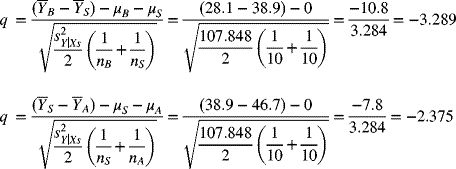
\begin{array}{l} q & = & \frac{({\bar{Y}}_{B} - {\bar{Y}}_{S}) - μ_{B} - μ_{S}}{\sqrt{\frac{s_{Y | X s}^{2}}{2} (\frac{1}{n_{B}} + \frac{1}{n_{S}})}} = \frac{(28.1 - 38.9) - 0}{\sqrt{\frac{107.848}{2} (\frac{1}{10} + \frac{1}{10})}} = \frac{- 10.8}{3.284} = - 3.289 \\ q & = & \frac{({\bar{Y}}_{S} - {\bar{Y}}_{A}) - μ_{S} - μ_{A}}{\sqrt{\frac{s_{Y | X s}^{2}}{2} (\frac{1}{n_{S}} + \frac{1}{n_{A}})}} = \frac{(38.9 - 46.7) - 0}{\sqrt{\frac{107.848}{2} (\frac{1}{10} + \frac{1}{10})}} = \frac{- 7.8}{3.284} = - 2.375 \end{array}

The critical value for these comparisons is 2.888. The absolute calculated value for BYPASS vs STENT is greater than the critical value, but the absolute calculated value for STENT vs ANGIO is less than the critical value. BYPASS is significantly different from ANGIO and STENT, but ANGIO and STENT are not significantly different from each other.

Now, let us recognize that we have two drugs (Drug 1 and Drug 2) that are intended to reduce the rate of re-stenosis post-treatment. Suppose we randomly assign half the persons in each of the three treatment groups to one of those drugs (i.e., five in each group assigned one of the drugs).

Now, we have six groups of dependent variable values instead of three. More importantly, we have two factors (i.e., characteristics) that are used to create those groups. One of these is treatment group and the other is drug group. As before, treatment group has three categories: BYPASS, STENT, and ANGIO. Drug group has two categories: DRUG 1 and DRUG 2. Both factors together account for 3 × 2= 6 groups of dependent variable values.

When the groups of dependent variable values are specified by more than one characteristic, we can separate the variation between the groups into main effects and interactions. The main effects address the variation between groups specified by just one factor. Interactions address the consistency of the main effects. Use the “ANOVA: Two-Factor With Replication” analysis tool to consider both treatment and drug.

When we have only one characteristic that divides the dependent variable into groups (i.e., one-way ANOVA), this is the only null hypothesis we can test. When we have more than one factor, we can test null hypotheses about the main effects and interactions.

10.20. At which of those results should we look first? Why?

We should first look at the interaction using “ANOVA: Two Factor With Replication” analysis tool. If it is statistically significant, we will not interpret the main effects.

10.21. Interpret the main effects and interactions in the output from Excel

The interaction is not significant, so we can look at the main effects. Both main effects have P-values less than 0.05.

There are only two categories of drug, so rejection of the null hypothesis for that main effect leads to acceptance of the alternative hypothesis that those two means are not equal. Rejection of the null hypothesis for the main effect of treatment group, however, does not tell us which means are different from which other means. Just like in one-way ANOVA, we need to perform a posterior test to see which means are significantly different.

For this set of data, we concluded there was no interaction between treatment group and drug. If we look at the means for those six groups (in the table), we see that, regardless of which treatment group to which people were assigned, those who received Drug 1 had a mean percent stenosis that was about 11% greater than those who received Drug 2. Also, the highest percent stenosis was seen among persons who had angioplasty and the lowest percent stenosis was seen among persons who had bypass surgery, regardless of which drug they received. This is what we imply when we say there is not an interaction between factors; the relationship between categories of one factor is not influenced by categories of another factor.

To see what interaction looks like, let us analyze a new dataset (WBEXP10_22).

**Table 10.3** Excel dataset for drugs and procedures effect on percent stenosis with interaction.

Let use the “ANOVA: Two-Factor With Replication” analysis tool to analyze the new dataset.

10.22. Interpret the main effects and interactions in the output from the “ANOVA: Two-Factor With Replication” analysis tool

Now, the interaction is statistically significant, so we cannot interpret the main effects.

Next, let us represent these in data in an ANCOVA. To do that, we need to add the indicator variables for the treatment groups. We could use either of the indicators that we discussed in the text. The only rule is that the numeric values need to be confined to zero, plus one, and, perhaps, minus one. We select from these numeric values since they have qualitative, rather than quantitative natures. For now, let us suppose we are interested in comparing the mean percent stenosis estimate for persons who received a stent to the mean percent stenosis estimate for persons who had bypass surgery and to the mean percent stenosis estimate for persons who had angioplasty.

10.23. How should we define the indicator variables to facilitate those comparisons?

When we want to compare all groups to one specific group, we need to use 0, 1 indicator variables with the comparison group assigned zero for all the indicator variables.

The data now look like those in Table 10.4 (WBEXP10_24).

**Table 10.4** Excel dataset for drugs and procedures effect on percent stenosis. The nominal independent variables are represented with 0/1 indicator variables.

10.24. Analyze those data and interpret them

The following output is what we receive from the “Regression” Analysis Tool when we include serum cholesterol (CHOL) as a continuous independent variable, and indicator variables for the treatment groups. ANGIO is an indicator variable that is equal to one if the person had angioplasty and equal to zero otherwise. BYPASS is an indicator variable that is equal to one if the person had bypass surgery and equal to zero otherwise.

Since the indicator variables for BYPASS and ANGIO are significantly different from zero, the intercepts for BYPASS and ANGIO are significantly different from the intercept for stent. Since the regression coefficient for cholesterol is positive and significant, percent stenosis increases as serum cholesterol increases.

10.25. Represent those relationships graphically

Those three regression lines have the same slope (i.e., they are parallel). To allow the lines to have different slopes, we need to add interactions between each of the indicator variables and the continuous independent variable to the regression equation. With interactions, the data are as in Table 10.5 (WBEXP10_26).

Figure depicting a scatterplot between percent stenosis on the y-axis (on a scale of 0–70) and serum cholesterol on the x-axis (on a scale of 0–500). The shaded circles represent angio, shaded squares represent bypass, and shaded diamonds represent stent. The three regression lines formed are parallel to each other. — **Figure 10.1** Scatter plot of the results in Example 10.24.

**Table 10.5** Excel dataset for drugs, procedures, and serum cholesterol effect on percent stenosis. The nominal independent variables are represented with 0/1 indicator variables and interactions.

10.26. Analyze and interpret those data

The slope of CHOL for BYPASS is lower than the slope of CHOL for STENT, The slope for ANGIO is higher than the slope for STENT.

10.27. Represent those data graphically

Since an interaction is created by multiplying two (or more) independent variables together, the interaction is highly correlated with those variables. Thus, there is the potential for collinearity. One effect of this is that it is harder to interpret the regression coefficients for the independent variables that are part of the interaction as long as the interaction is in the regression equation. For this reason, interactions can be dropped from the regression equation if they are not statistically significant.

10.28. Analyze and interpret the data with the interaction between ANGI and cholesterol removed. What happens? Why?

The P-values got smaller because some collinearity was removed.

Exercises

10.1. Suppose we are interested in the relationship between dietary sodium intake (NA) and diastolic blood pressure (DBP). To investigate this relationship, we measure both for a sample of 40 persons. Because DBP and NA both increase with age, we decide to control for age in our analysis. The data for this question are in the Excel file: EXR10_1. Based on those observations, which of the following is closest to the percent variation in DBP that is explained by the combination of NA and age?

14.4%
24.3%
30.7%
38.0%
55.4%

10.2. Suppose we are interested in which blood chemistry measurements are predictive of urine creatinine. To investigate this, we identify 100 persons and measure their urine creatinine levels. We also measure serum creatinine, blood urea nitrogen (BUN), and serum potassium. These data are in the Excel file called EXR10_2. Use Excel to determine the percent of the variation in urine creatinine that is explained by the combination of serum creatinine, BUN, and serum potassium. Which of the following is closest to that value?

73.3%
69.3%
53.7%
48.0%
43.0%

10.3. Suppose we are interested in the relationship between dietary sodium intake (NA) and diastolic blood pressure (DBP). To investigate this relationship, we measure both for a sample of 40 persons. Because DBP and NA both increase with age, we decide to control for age in our analysis. The data for this question is in the Excel file: EXR10_1. Based on those observations, test the null hypothesis that the combination of NA and age does not help estimate DBP, versus the alternative hypothesis that it does. If you allow a 5% chance of making a type I error, which of the following is the best conclusion to draw?

Reject both the null and alternative hypotheses
Accept both the null and alternative hypotheses
Reject the null hypothesis and accept the alternative hypothesis
Accept the null hypothesis and reject the alternative hypothesis
It is best not to draw a conclusion about the null and alternative hypotheses from these observations

10.4. Suppose we are interested in which blood chemistry measurements are predictive of urine creatinine. To investigate this, we identify 100 persons and measure their urine creatinine levels. We also measure serum creatinine, blood urea nitrogen (BUN), and serum potassium. These data are in the Excel file called EXR10_2. Use Excel to test the null hypothesis that the combination of serum creatinine, BUN, and serum potassium do not help estimate urine creatinine versus the alternative hypothesis that they do help. If you allow a 5% chance of making a type I error, what is the best conclusion to draw?

Reject both the null and alternative hypotheses
Accept both the null and alternative hypotheses
Reject the null hypothesis and accept the alternative hypothesis
Accept the null hypothesis and reject the alternative hypothesis
It is best not to draw a conclusion about the null and alternative hypotheses from these observations

10.5. Suppose we are interested in the relationship between dietary sodium intake (NA) and diastolic blood pressure (DBP). To investigate this relationship, we measure both for a sample of 40 persons. Because DBP and NA both increase with age, we decide to control for age in our analysis. The data for this question is in the Excel file: EXR10_1. Based on those observations, test the null hypothesis that the regression coefficient for NA, controlling for AGE, is equal to zero in the population versus the alternative hypothesis that it is not equal to zero. If you allow a 5% chance of making a type I error, which of the following is the best conclusion to draw?

Reject both the null and alternative hypotheses
Accept both the null and alternative hypotheses
Reject the null hypothesis and accept the alternative hypothesis
Accept the null hypothesis and reject the alternative hypothesis
It is best not to draw a conclusion about the null and alternative hypotheses from these observations

10.6. Suppose we are interested in which blood chemistry measurements are predictive of urine creatinine. To investigate this, we identify 100 persons and measure their urine creatinine levels. We also measure serum creatinine, blood urea nitrogen (BUN), and serum potassium. These data are in the Excel file called EXR10_2. Use Excel to test the null hypothesis that the regression coefficient for serum creatinine, when controlling for BUN and serum potassium, is equal to zero versus the alternative hypothesis that it is not equal to zero. If you allow a 5% chance of making a type I error, what is the best conclusion to draw?

Reject both the null and alternative hypotheses
Accept both the null and alternative hypotheses
Reject the null hypothesis and accept the alternative hypothesis
Accept the null hypothesis and reject the alternative hypothesis
It is best not to draw a conclusion about the null and alternative hypotheses from these observations

10.7. Suppose we are interested in the relationship between dietary sodium intake (NA) and diastolic blood pressure (DBP). To investigate this relationship, we measure both for a sample of 40 persons. Because DBP and NA both increase with age, we decide to control for age in our analysis. The data for this question are in the Excel file: EXR10_1. Based on those observations, which of the following independent variables contributes the most to the estimate of DBP, controlling for the other independent variables?

AGE
NA
They both contribute about the same to estimation of DBP

10.8. Suppose we are interested in which blood chemistry measurements are predictive of urine creatinine. To investigate this, we identify 100 persons and measure their urine creatinine levels. We also measure serum creatinine, blood urea nitrogen (BUN), and serum potassium. These data are in the Excel file called EXR10_2. Use Excel to determine which of the independent variables contributes the most to estimation of urine creatinine, while controlling for the other independent variables?

Serum creatinine
BUN
Serum potassium
They all contribute about the same to estimation of urine creatinine

10.9. Suppose we are interested in the survival time for persons with cancer of various organs. To investigate this, we identify 64 persons who died with cancer as the primary cause of death and record the period of time from their initial diagnosis to their death (in days). Those data are in the Excel file EXR10_3. Based on those data, test the null hypothesis that all five means are equal to the same value in the population versus the alternative that they are not all equal. If you allow a 5% chance of making a type I error, which of the following is the best conclusion to draw?

Reject both the null and alternative hypotheses
Accept both the null and alternative hypotheses
Reject the null hypothesis and accept the alternative hypothesis
Accept the null hypothesis and reject the alternative hypothesis
It is best not to draw a conclusion about the null and alternative hypotheses from these observations

10.10. Suppose we are interested in force of head impact for crash dummies in vehicles with different driver safety equipment. To study this relationship, we examine the results for 175 tests. Those data are in the Excel file: EXR10_4. Based on those data, test the null hypothesis that all four means are equal to the same value in the population versus the alternative that they are not all equal. If you allow a 5% chance of making a type I error, which of the following is the best conclusion to draw?

Reject both the null and alternative hypotheses
Accept both the null and alternative hypotheses
Reject the null hypothesis and accept the alternative hypothesis
Accept the null hypothesis and reject the alternative hypothesis
It is best not to draw a conclusion about the null and alternative hypotheses from these observations

10.11. Suppose we are interested in survival times for persons with cancer of various organs. To investigate this, we identify 64 persons who died with cancer as the primary cause of death and record the period of time from their initial diagnosis to their death (in days). Those data are in the Excel file: EXR10_3. Based on those data, perform tests comparing two means at a time in a way that avoids problems with multiple comparisons. If you allow a 5% chance of making a type I error, which of the following is the best conclusion to draw?

All five means are significantly different from each other
The mean for Bronchus is significantly different from all of the other means
The mean for Bronchus is significantly different from all of the other means except the mean for Stomach
The mean for Breast is significantly different from all of the other means
The mean for Breast is significantly different from all of the other means except the mean for Ovary

10.12. Suppose we are interested in force of head impact for crash dummies in vehicles with different driver safety equipment. To study this relationship, we examine the results for 175 tests. Those data are in the Excel file: EXR10_4. Based on those data, perform tests comparing two means at a time in a way that avoids problems with multiple comparisons. If you allow a 5% chance of making a type I error, which of the following is the best conclusion to draw?

All four means are significantly different from each other
Manual Belt is significantly different from the other three means, but the other three means are not significantly different from each other
All four means are significantly different from each other except Airbag and Motorized belt
All four means are significantly different from each other except Motorized Belt and Passive Belt
All four means are significantly different from each other except Passive Belt and Manual Belt

10.13. In a study of clinical depression, patients were randomly assigned to one of four drug groups (three active drugs and a placebo) and to a cognitive therapy group (active versus placebo). The dependent variable is a difference between scores on a depression questionnaire. The results are in the Excel file: EXR10_5. Based on those data, test the null hypothesis of no interaction between drug and therapy versus the alternative hypothesis that there is interaction allowing a 5% chance of making a type I error. Which of the following is the best conclusion to draw?

Reject both the null and alternative hypotheses
Accept both the null and alternative hypotheses
Reject the null hypothesis and accept the alternative hypothesis
Accept the null hypothesis and reject the alternative hypothesis
It is best not to draw a conclusion about the null and alternative hypotheses from these observations

10.14. In a multicenter study of a new treatment for hypertension, patients at nine centers were randomly assigned to a new treatment or standard treatment. The dependent variable is a difference in diastolic blood pressure from a pretreatment value. The results are in the Excel file: EXR10_6. Based on those data, test the null hypothesis of no interaction between drug and center versus the alternative hypothesis that there is interaction allowing a 5% chance of making a type I error. Which of the following is the best conclusion to draw?

Reject both the null and alternative hypotheses
Accept both the null and alternative hypotheses
Reject the null hypothesis and accept the alternative hypothesis
Accept the null hypothesis and reject the alternative hypothesis
It is best not to draw a conclusion about the null and alternative hypotheses from these observations

10.15. In a study of clinical depression, patients were randomly assigned to one of four drug groups (three active drugs and a placebo) and to a cognitive therapy group (active versus no therapy). The dependent variable is a difference between scores on a depression questionnaire. The results are in the Excel file: EXR10_5. Based on those data, test the null hypothesis of no differences between drug groups versus the alternative hypothesis that there is a difference, ignoring the possibility of an interaction. Allowing a 5% chance of making a type I error, which of the following is the best conclusion to draw?

Reject both the null and alternative hypotheses
Accept both the null and alternative hypotheses
Reject the null hypothesis and accept the alternative hypothesis
Accept the null hypothesis and reject the alternative hypothesis
It is best not to draw a conclusion about the null and alternative hypotheses from these observations

10.16. In a multicenter study of a new treatment for hypertension, patients at nine centers were randomly assigned to a new treatment or standard treatment. The dependent variable is a difference in diastolic blood pressure from a pretreatment value. The results are in the Excel file: EXR10_6. Based on those data, test the null hypothesis of no difference between drugs versus the alternative hypothesis that there is a difference, ignoring the possibility of an interaction. If you allow a 5% chance of making a type I error, which of the following is the best conclusion to draw?

Reject both the null and alternative hypotheses
Accept both the null and alternative hypotheses
Reject the null hypothesis and accept the alternative hypothesis
Accept the null hypothesis and reject the alternative hypothesis
It is best not to draw a conclusion about the null and alternative hypotheses from these observations

10.17. In a study of clinical depression, patients were randomly assigned to one of four drug groups (three active drugs and a placebo) and to a cognitive therapy group (active versus no therapy). The dependent variable is a difference between scores on a depression questionnaire. The results are in the Excel file: EXR10_5. Based on those data, test the null hypothesis of no difference between therapy groups versus the alternative hypothesis that there is a difference, ignoring the possibility of an interaction. Allowing a 5% chance of making a type I error, which of the following is the best conclusion to draw?

Reject both the null and alternative hypotheses
Accept both the null and alternative hypotheses
Reject the null hypothesis and accept the alternative hypothesis
Accept the null hypothesis and reject the alternative hypothesis
It is best not to draw a conclusion about the null and alternative hypotheses from these observations

10.18. In a multicenter study of a new treatment for hypertension, patients at nine centers were randomly assigned to a new treatment or standard treatment. The dependent variable is a difference in diastolic blood pressure from a pretreatment value. The results are in the Excel file: EXR10_6. Based on those data, test the null hypothesis of no difference among centers in the population versus the alternative hypothesis that there is a difference, ignoring the possibility of an interaction. If you allow a 5% chance of making a type I error, which of the following is the best conclusion to draw?

Reject both the null and alternative hypotheses
Accept both the null and alternative hypotheses
Reject the null hypothesis and accept the alternative hypothesis
Accept the null hypothesis and reject the alternative hypothesis
It is best not to draw a conclusion about the null and alternative hypotheses from these observations

10.19. Suppose we are interested in the relationship between body mass index (BMI) and serum cholesterol (the dependent variable) controlling for gender (SEX = 1 for women and SEX = 0 for men). To study this relationship, we analyze data from 300 persons who participated in the Framingham Heart Study. Those data are in Excel file: EXR10_7. Analyze those data as an ANCOVA. From that output, do you think the slopes of the regression lines for men and women are different?

No, the slopes are the same
Yes, the slopes are different, but not significantly different
Yes, the slopes are different and they are significantly different

10.20. Suppose we are interested in the relationship between time since diagnosis of HIV and CD4 count. To investigate this relationship, we examine 1,151 HIV positive patients. In making this comparison, we control for gender (SEX = 1 for women and SEX = 0 for men). These data are in the Excel file: EXR10_8. Which of the following is the best description of the relationship between time since diagnosis and CD4 in the sample?

CD4 decreases with longer time since diagnosis for both men and women
CD4 decreases with longer time since diagnosis for women only
CD4 decreases with longer time since diagnosis for men only
CD4 decreases with longer time since diagnosis for men and increases for women
CD4 decreases with longer time since diagnosis for women and increases for men