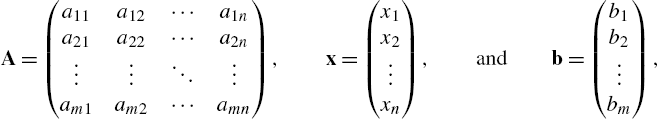
Matrices and Vectors: Topics from Linear Algebra and Vector Calculus
Keywords
Linear algebra; Eigenvalues; Eigenvectors; Vector calculus; Engineering applications; Linear programming; Photo special effects; Applying effects to photos and figures
5.1 Nested Lists: Introduction to Matrices, Vectors, and Matrix Operations
5.1.1 Defining Nested Lists, Matrices, and Vectors
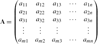
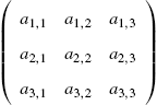
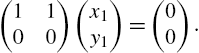
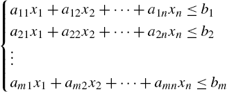
In Mathematica, a matrix is a list of lists where each list represents a row of the matrix. Therefore, the ![]() matrix
matrix
is entered with
A={{a11,a12,...,a1n},{a21,a22,...,a2n},...,{am1,am2,...amn}}.
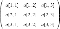
For example, to use Mathematica to define m to be the matrix ![]() enter the command
enter the command
m={{a11,a12},{a21,a22}}.
The command m=Array[a,{2,2}] produces a result equivalent to this. Once a matrix A has been entered, it can be viewed in the traditional row-and-column form using the command MatrixForm[A]. You can quickly construct ![]() matrices by clicking on the
matrices by clicking on the ![]() button from the BasicMathInput palette, which is accessed by going to Palettes followed by BasicMathInput.
button from the BasicMathInput palette, which is accessed by going to Palettes followed by BasicMathInput.
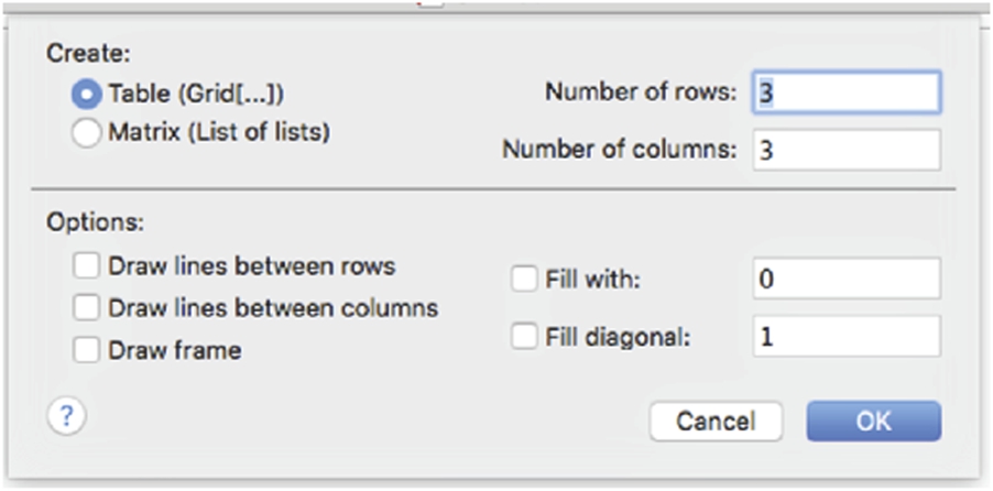
Alternatively, you can construct matrices of any dimension by going to the Mathematica menu under Insert and selecting Create Table/Matrix/Palette...
Use Part, ([[...]]) to select elements of lists. Because of the construct of the matrix, m[[i]] returns the ith row of M. The transpose of M, ![]() , is the matrix obtained by interchanging the rows and columns of matrix M. Thus, to extract the ith column of M, use the commands mt=Transpose[m] followed by mt[[i]].
, is the matrix obtained by interchanging the rows and columns of matrix M. Thus, to extract the ith column of M, use the commands mt=Transpose[m] followed by mt[[i]].

The resulting pop-up window allows you to create tables, matrices, and palettes. To create a matrix, select Matrix, enter the number of rows and columns of the matrix, and select any other options. Pressing the OK button places the desired matrix at the position of the cursor in the Mathematica notebook.
Example 5.1
Use Mathematica to define the matrices  and
and ![]() .
.
Solution
In this case, both ![]() and Array[a,{3,3}] produce equivalent results when we define matrixa to be the matrix
and Array[a,{3,3}] produce equivalent results when we define matrixa to be the matrix
The commands MatrixForm or TableForm are used to display the results in traditional matrix form.
![]()
![]()
![]()
![]()
![]()
![]()
![]()
![]()
![]()
We may also use Mathematica to define non-square matrices.
![]()
![]()
![]()
Equivalent results would have been obtained by entering ![]() . □
. □
More generally the commands Table[f[i,j],{i,imax},{j,jmax}] and Array[f,{imax,jmax}] yield nested lists corresponding to the ![]() matrix
matrix
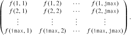
Table[f[i,j],{i,imin,imax,istep},{j,jmin,jmax,jstep}] returns the list of lists
{{f[imin,jmin],f[imin,jmin+jstep],...,f[imin,jmax]},
     {f[imin+istep,jmin],...,f[imin+istep,jmax]},
          ...,{f[imax,jmin],...,f[imax,jmax]}}
and the command
Table[f[i,j,k,...],{i,imin,imax,istep},{j,jmin,jmax,jstep},
     {k,kmin,kmax,kstep},...]
calculates a nested list; the list associated with i is outermost. If istep is omitted, the stepsize is one.
Example 5.2
Define C to be the ![]() matrix
matrix ![]() , where
, where ![]() , the entry in the ith row and jth column of C, is the numerical value of
, the entry in the ith row and jth column of C, is the numerical value of ![]() .
.
Solution
After clearing all prior definitions of c, if any, we define c[i,j] to be the numerical value of ![]() and then use Array to compute the
and then use Array to compute the ![]() matrix matrixc.
matrix matrixc.
![]()
![]()
![]()
![]()
![]()
![]()
![]()
![]()
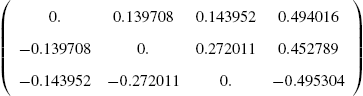
Mathematica provides several functions to help visualize a matrix. These commands include MatrixPlot, ArrayPlot, ReliefPlot, and ListDensityPlot. These commands have many of the same options as Plot.
Each produces a slightly different result. To achieve the best result, we suggest that you try each and then adjust the options to finalize your result. In Fig. 5.1, we show the results of each command for matrixc.

![]()
![]()
![]()
![]()
![]()
![]()
![]()
![]() □
□
Example 5.3
Define the matrix 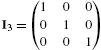 .
.
Solution
The matrix ![]() is the
is the ![]() identity matrix. Generally, the
identity matrix. Generally, the ![]() matrix with 1's on the diagonal and 0's elsewhere is the
matrix with 1's on the diagonal and 0's elsewhere is the ![]() identity matrix. The command IdentityMatrix[n] returns the
identity matrix. The command IdentityMatrix[n] returns the ![]() identity matrix.
identity matrix.
![]()
![]()
The same result is obtained by going to Insert under the Mathematica menu and selecting Table/Matrix/ followed by New.... We then check Matrix, Fill with: 0 and Fill diagonal: 1.
Pressing the OK button inserts the ![]() identity matrix at the location of the cursor.
identity matrix at the location of the cursor.

![]() □
□
In Mathematica, a vector is a list of numbers and, thus, is entered in the same manner as lists. For example, to use Mathematica to define the row vector vectorv to be ![]() enter vectorv={v1,v2,v3}. Similarly, to define the column vector vectorv to be
enter vectorv={v1,v2,v3}. Similarly, to define the column vector vectorv to be ![]() enter vectorv={v1,v2,v3} or vectorv={{v1},{v2},{v3}}.
enter vectorv={v1,v2,v3} or vectorv={{v1},{v2},{v3}}.
Generally, with Mathematica you do not need to distinguish between row and column vectors: Mathematica usually performs computations with vectors and matrices correctly as long as the computations are well-defined.
Example 5.4
Define the vector  , vectorv to be the vector
 ![]() and zerovec to be the vector
and zerovec to be the vector ![]() .
.
Solution
To define w, we enter
![]()
![]()
or
![]()

To define vectorv, we use Array.
![]()
![]()
Equivalent results would have been obtained by entering ![]() . To define zerovec, we use Table.
. To define zerovec, we use Table.
![]()
![]()
The same result is obtained by going to Insert under the Mathematica menu and selecting Table/Matrix to create the zero vector.
![]()
![]() □
□
5.1.2 Extracting Elements of Matrices
For the ![]() matrix
matrix ![]() defined earlier, m[[1]] yields the first element of matrix m which is the list
defined earlier, m[[1]] yields the first element of matrix m which is the list ![]() or the first row of m; m[[2,1]] yields the first element of the second element of matrix m which is
or the first row of m; m[[2,1]] yields the first element of the second element of matrix m which is ![]() . In general, if m is an
. In general, if m is an ![]() matrix, m[[i,j]] or Part[m,i,j] returns the unique element in the ith row and jth column of m. More specifically, m[[i,j]] yields the jth part of the ith part of m; list[[i]] or Part[list,i] yields the ith part of list; list[[i,j]] or Part[list,i,j] yields the jth part of the ith part of list, and so on.
matrix, m[[i,j]] or Part[m,i,j] returns the unique element in the ith row and jth column of m. More specifically, m[[i,j]] yields the jth part of the ith part of m; list[[i]] or Part[list,i] yields the ith part of list; list[[i,j]] or Part[list,i,j] yields the jth part of the ith part of list, and so on.
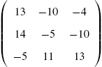
Example 5.5
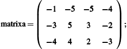
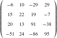
Define mb to be the matrix 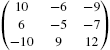 . (a) Extract the third row of mb. (b) Extract the element in the first row and third column of mb. (c) Display mb in traditional matrix form.
Solution
We begin by defining mb. mb[[i,j]] yields the (unique) number in the ith row and jth column of mb. Observe how various components of mb (rows and elements) can be extracted and how mb is placed in MatrixForm.
![]()
![]()
![]()
![]()
![]()
−9 □
If m is a matrix, the ith row of m is extracted with m[[i]]. The command Transpose[m] yields the transpose of the matrix m, the matrix obtained by interchanging the rows and columns of m. We extract columns of m by computing Transpose[m] and then using Part to extract rows from the transpose. Namely, if m is a matrix, Transpose[m][[i]] extracts the ith row from the transpose of m which is the same as the ith column of m.
Alternatively, if A is ![]() (rows × columns) the ith column of A is the vector that consists of the ith part of each row of the matrix so given an i-value Table[A[[j,i]],{j,1,n}] returns the ith column of A.
(rows × columns) the ith column of A is the vector that consists of the ith part of each row of the matrix so given an i-value Table[A[[j,i]],{j,1,n}] returns the ith column of A.
Example 5.6
Extract the second and third columns from  .
.
Solution
We first define matrixa and then use Transpose to compute the transpose of matrixa, naming the result ta, and then displaying ta in MatrixForm.
![]()
![]()
![]()
![]()
![]()
Next, we extract the second column of matrixa using Transpose together with Part ([[...]]). Because we have already defined ta to be the transpose of matrixa, entering ta[[2]] would produce the same result.
![]()
![]()
To extract the third column, we take advantage of the fact that we have already defined ta to be the transpose of matrixa. Entering Transpose[matrixa][[3]] produces the same result.
![]()
![]()
You can also use Take to extract elements of lists and matrices. Entering
![]()
![]()
![]()
returns the first two rows of matrixa because the first two parts of matrixa are the lists corresponding to those rows. Similarly,
![]()
![]()
![]()
![]()
returns the second row while
![]()
![]()
![]()
returns the second and third rows. □
The example illustrates that Take[list,n] returns the first n elements of list; Take[list,{n}] returns the nth element of list; Take[list,{n1,n2,...}] returns the ![]() st,
st, ![]() nd, ... elements of list, and so on.
nd, ... elements of list, and so on.
5.1.3 Basic Computations with Matrices
Mathematica performs all of the usual operations on matrices. Matrix addition (![]() ), scalar multiplication (
), scalar multiplication (![]() ), matrix multiplication (when defined) (AB), and combinations of these operations are all possible. The transpose of A,
), matrix multiplication (when defined) (AB), and combinations of these operations are all possible. The transpose of A, ![]() , is obtained by interchanging the rows and columns of A and is computed with the command Transpose[A]. If A is a square matrix, the determinant of A is obtained with Det[A].
, is obtained by interchanging the rows and columns of A and is computed with the command Transpose[A]. If A is a square matrix, the determinant of A is obtained with Det[A].
If A and B are ![]() matrices satisfying
matrices satisfying ![]() , where I is the
, where I is the ![]() matrix with 1's on the diagonal and 0's elsewhere (the
matrix with 1's on the diagonal and 0's elsewhere (the ![]() identity matrix), B is called the inverse of A and is denoted by
identity matrix), B is called the inverse of A and is denoted by ![]() . If the inverse of a matrix A exists, the inverse is found with Inverse[A]. Thus, assuming that
. If the inverse of a matrix A exists, the inverse is found with Inverse[A]. Thus, assuming that ![]() has an inverse (
has an inverse (![]() ), the inverse is
), the inverse is ![]() .
.
This easy-to-remember formula for finding the inverse of a ![]() matrix is sometimes called “the handy two-by-two inverse trick” by instructors and students.
matrix is sometimes called “the handy two-by-two inverse trick” by instructors and students.
![]()
![]()
Example 5.7
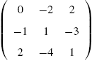
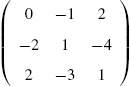
Let  and
and 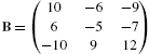 . Compute
(a) ![]() ; (b)
; (b) ![]() ; (c) the inverse of AB; (d) the transpose of
; (c) the inverse of AB; (d) the transpose of ![]() ; and (e)
; and (e) ![]() .
.
Solution
We enter ma (corresponding to A) and mb (corresponding to B) as nested lists where each element corresponds to a row of the matrix. We suppress the output by ending each command with a semi-colon.
![]()
![]()
Entering
![]()
adds matrix ma to mb and expresses the result in traditional matrix form. Entering
![]()
subtracts four times matrix ma from mb and expresses the result in traditional matrix form. Entering
![]()
computes the inverse of the matrix product AB. Similarly, entering
![]()
computes the transpose of ![]() and entering
and entering
![]()
190
computes the determinant of A. □
Example 5.8
Compute AB and BA if  and
and  .
.
Solution
Because A is a ![]() matrix and B is a
matrix and B is a ![]() matrix, AB is defined and is a
matrix, AB is defined and is a ![]() matrix. We define matrixa and matrixb with the following commands.
matrix. We define matrixa and matrixb with the following commands.

We then compute the product, naming the result ab, and display ab in MatrixForm.
![]()
![]()

However, the matrix product BA is not defined and Mathematica produces error messages, which are not displayed here, when we attempt to compute it.
![]()
![]() □
□
Special attention must be given to the notation that must be used in taking the product of a square matrix with itself. The following example illustrates how Mathematica interprets the expression (matrixb)^n. The command (matrixb)^n raises each element of the matrix matrixb to the nth power. The command MatrixPower is used to compute powers of matrices.
Example 5.9
Let  . (a) Compute
 ![]() and
and ![]() . (b) Cube each entry of B.
. (b) Cube each entry of B.
Solution
After defining B, we compute ![]() . The same results would have been obtained by entering MatrixPower[matrixb,2].
. The same results would have been obtained by entering MatrixPower[matrixb,2].
![]()
![]()
![]()
Next, we use MatrixPower to compute ![]() . The same results would be obtained by entering matrixb.matrixb.matrixb.
. The same results would be obtained by entering matrixb.matrixb.matrixb.
![]()
Last, we cube each entry of B with ^.
![]()
 □
□
If ![]() , the inverse of A can be computed using the formula
, the inverse of A can be computed using the formula
where ![]() is the transpose of the cofactor matrix.
is the transpose of the cofactor matrix.
The cofactor matrix, ![]() , of A is the matrix obtained by replacing each element of A by its cofactor.
, of A is the matrix obtained by replacing each element of A by its cofactor.
If A has an inverse, reducing the matrix ![]() to reduced row echelon form results in
to reduced row echelon form results in ![]() . This method is often easier to implement than (5.1).
. This method is often easier to implement than (5.1).
Example 5.10
Calculate ![]() if
if 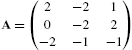 .
.
Solution
After defining A and 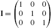 , we compute
 ![]() , so
, so ![]() exists.
exists.
![]()
![]()
![]()
![]()
![]()
12
Join[a,b,n] concatenates lists a and b at level n. For matrices the level one objects (capa[[i]]) are the rows; the level two objects (capa[[i,j]]) are the entries. Thus, Join[capa,i3] returns the matrix ![]() while Join[capa,i3,2] forms the matrix
while Join[capa,i3,2] forms the matrix ![]() .
.
![]()
![]()
![]()
![]()
![]()

We then use RowReduce to reduce ![]() to row echelon form.
to row echelon form.
![]()
![]()
![]()
![]()
![]()
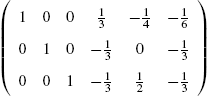
The result indicates that 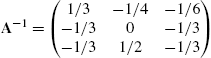 . □
. □
5.1.4 Basic Computations with Vectors
5.1.4.1 Basic Operations on Vectors
Computations with vectors are performed in the same way as computations with matrices.
Example 5.11
Let  and
and  . (a) Calculate
 ![]() and
and ![]() . (b) Find a unit vector with the same direction as v and a unit vector with the same direction as w.
. (b) Find a unit vector with the same direction as v and a unit vector with the same direction as w.
Solution
We begin by defining v and w and then compute ![]() and
and ![]() .
.
![]()
![]()
![]()
![]()
![]()
0
The norm of the vector  is
is
The command Norm[v] returns the norm of the vector v.
If k is a scalar, the direction of ![]() is the same as the direction of v. Thus, if v is a nonzero vector, the vector
is the same as the direction of v. Thus, if v is a nonzero vector, the vector ![]() has the same direction as v and because
has the same direction as v and because ![]() ,
, ![]() is a unit vector. First, we compute
is a unit vector. First, we compute ![]() with Norm. We then compute
with Norm. We then compute ![]() , calling the result uv, and
, calling the result uv, and ![]() . The results correspond to unit vectors with the same direction as v and w, respectively.
. The results correspond to unit vectors with the same direction as v and w, respectively.
![]()
![]()
![]()
![]()
![]()
1
![]()
![]() □
□
5.1.4.2 Basic Operations on Vectors in 3-Space
We review the elementary properties of vectors in 3-space. Let
and
be vectors in space.
1. u and v are equal if and only if their components are equal:
2. The length (or norm) of u is
3. If c is a scalar (number),
4. The sum of u and v is defined to be the vector
5. If ![]() , a unit vector with the same direction as u is
, a unit vector with the same direction as u is
6. u and v are parallel if there is a scalar c so that ![]() .
.
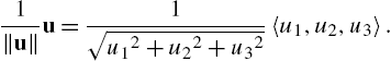
7. The dot product of u and v is
If θ is the angle between u and v,
Consequently, u and v are orthogonal if ![]() .
.
8. The cross product of u and v is
You should verify that ![]() and
and ![]() . Hence,
. Hence, ![]() is orthogonal to both u and v.
is orthogonal to both u and v.
Topics from linear algebra (including determinants, which were mentioned previously) are discussed in more detail in the next sections. For now, we illustrate several of the basic operations listed above: u.v and Dot[u,v] compute ![]() ; Cross[u,v] computes
; Cross[u,v] computes ![]() .
.
In space, the standard unit vectors are ![]() ,
, ![]() , and
, and ![]() . With the exception of the cross product, the vector operations discussed here are performed in the same way for vectors in the plane as they are in space. In the plane, the standard unit vectors are
. With the exception of the cross product, the vector operations discussed here are performed in the same way for vectors in the plane as they are in space. In the plane, the standard unit vectors are ![]() and
and ![]() .
.
Example 5.12
Let ![]() and
and ![]() . Calculate (a)
. Calculate (a) ![]() , (b)
, (b) ![]() , (c)
, (c) ![]() , and (d)
, and (d) ![]() . (e) Find the angle between u and v. (f) Find unit vectors with the same direction as u, v, and
. (e) Find the angle between u and v. (f) Find unit vectors with the same direction as u, v, and ![]() .
.
Solution
We begin by defining ![]() and
and ![]() . Notice that to define
. Notice that to define ![]() with Mathematica, we use the form
with Mathematica, we use the form
u={u1,u2,u3}.
We illustrate the use of Dot and Cross to calculate (a)–(d).
Similarly, to define ![]() , we use the form u={u1,u2}.
, we use the form u={u1,u2}.
![]()
![]()
![]()
−2
![]()
−2
![]()
![]()
![]()
![]()
![]()
![]()
We use the formula ![]() to find the angle θ between u and v.
to find the angle θ between u and v.
![]()
![]()
![]()
1.6437
Unit vectors with the same direction as u, v, and ![]() are found next.
are found next.
![]()
![]()
![]()
![]()
![]()
![]()
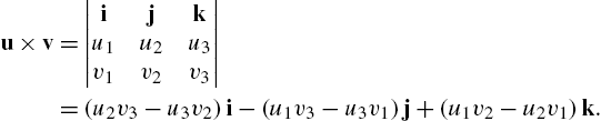
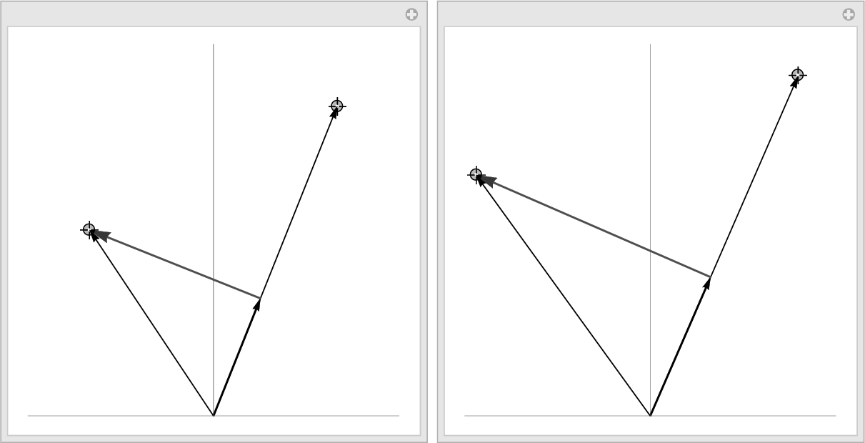
We can graphically confirm that these three vectors are orthogonal by graphing all three vectors with the graphics primitive Arrow together with Graphics3D. We show the vectors in Fig. 5.2.

![]()
![]()
In the plot, the vectors may not appear to be orthogonal (perpendicular) as expected because of the aspect ratio and viewing angles of the graphic. □
With the exception of the cross product, the calculations described above can also be performed on vectors in the plane.
Example 5.13
Solution
First, we define ![]() and
and ![]() and then compute
and then compute ![]() .
.
![]()
![]()
![]()
![]()
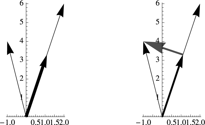
Next, we graph u, v, and ![]() together using Arrow, Show and GraphicsRow in Fig. 5.3.
together using Arrow, Show and GraphicsRow in Fig. 5.3.
![]()
![]()
![]()
![]()
![]()
![]()
![]()
![]()
![]()
In the graph, notice that ![]() and the vector
and the vector ![]() is perpendicular to v.
is perpendicular to v.
With the following, we use Manipulate to generalize the example. See Fig. 5.4.
![]()
![]()
![]()
![]()
![]()
![]()
![]()
![]()
![]()
![]() □
□
If you only need to display a two-dimensional array in row-and-column form, it is easier to use Grid rather than Table together with TableForm or MatrixForm.

For a list of all the options associated with Grid, enter Options[Grid].
Thus,
![]()
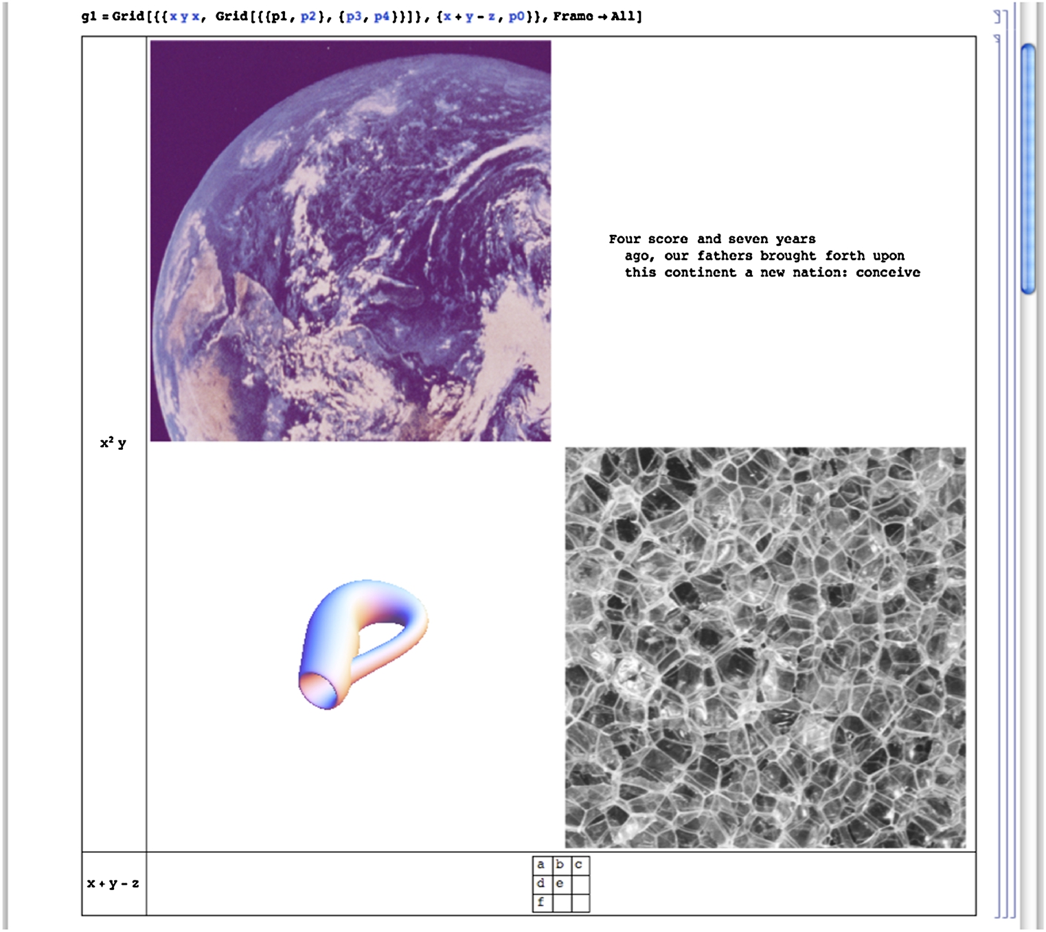
creates a basic grid. The first row consists of the entries a, b, and c; the second row d and e; and the third row f. See Fig. 5.5. Note that elements of grids can be any Mathematica object, including other grids.

You can create quite complex arrays with Grid. For example, elements of grids can be any Mathematica object, including grids.
In the following, we use ExampleData to generate several typical Mathematica objects.
![]()
![]()
![]()
![]()
Using our first grid, the above, and a few more strings we create a more sophisticated grid in Fig. 5.6.
![]()
5.2 Linear Systems of Equations
5.2.1 Calculating Solutions of Linear Systems of Equations
To solve the system of linear equations ![]() , where A is the coefficient matrix, b is the known vector and x is the unknown vector, we often proceed as follows: if
, where A is the coefficient matrix, b is the known vector and x is the unknown vector, we often proceed as follows: if ![]() exists, then
exists, then ![]() so
so ![]() .
.
Mathematica offers several commands for solving systems of linear equations, however, that do not depend on the computation of the inverse of A. The command
Solve[{eqn1,eqn2,...,eqnm},{var1,var2,...,varn}]
solves an ![]() system of linear equations (m equations and n unknown variables). Note that both the equations as well as the variables are entered as lists. If one wishes to solve for all variables that appear in a system, the command Solve[{eqn1,eqn2,...eqnn}] attempts to solve eqn1, eqn2, ..., eqnn for all variables that appear in them. (Remember that a double equals sign (==) must be placed between the left and right-hand sides of each equation.)
system of linear equations (m equations and n unknown variables). Note that both the equations as well as the variables are entered as lists. If one wishes to solve for all variables that appear in a system, the command Solve[{eqn1,eqn2,...eqnn}] attempts to solve eqn1, eqn2, ..., eqnn for all variables that appear in them. (Remember that a double equals sign (==) must be placed between the left and right-hand sides of each equation.)
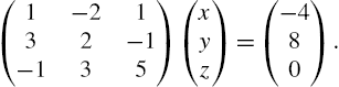
Example 5.14
Solve the matrix equation  .
.
Solution
The solution is given by 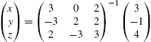 . We proceed by defining matrixa and b and then using Inverse to calculate Inverse[matrixa].b naming the resulting output {x,y,z}.
![]()
![]()
![]()
![]()
We verify that the result is the desired solution by calculating matrixa.{x,y,z}. Because the result of this procedure is ![]() , we conclude that the solution to the system is
, we conclude that the solution to the system is  .
.
![]()
![]()
We note that this matrix equation is equivalent to the system of equations
which we are able to solve with Solve. (Note that Thread[{f1,f2,...}={g1,g2,...}] returns the system of equations {f1==g1,f2==g2,...}.)
![]()
![]()
![]()
![]()
![]()
Shortly, we will discuss using row reduction to solve systems of equations. For now, we remark that given the augmented matrix for a system, ![]() , RowReduce reduces
, RowReduce reduces ![]() to reduced row echelon form so that you can see the solution(s) to the linear system, if any.
to reduced row echelon form so that you can see the solution(s) to the linear system, if any.
![]()
![]() □
□
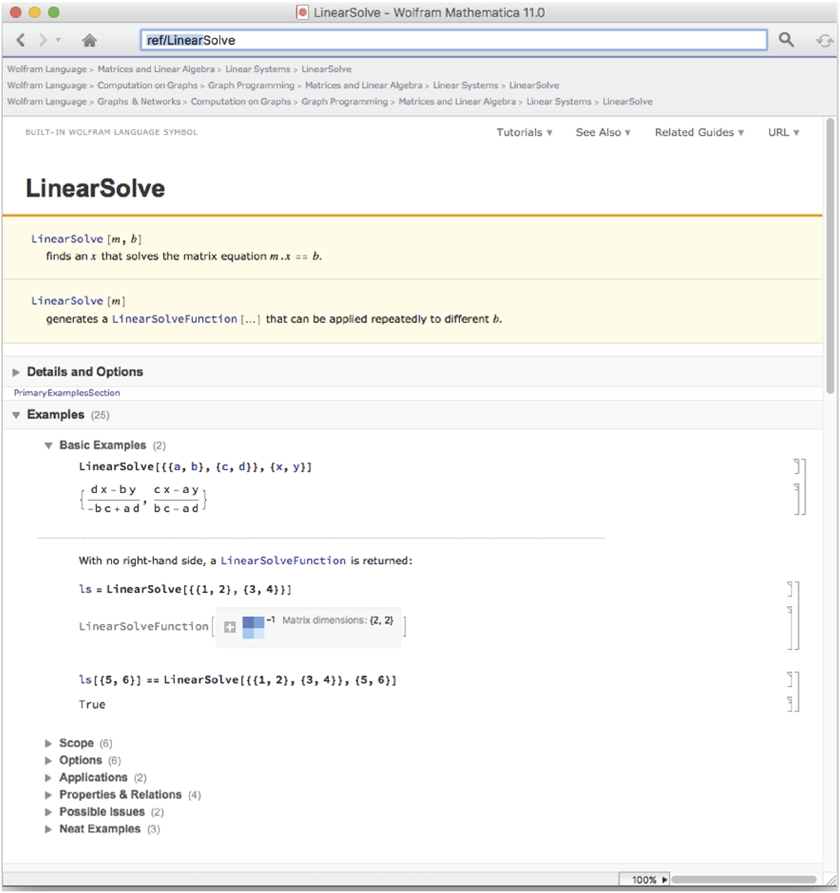
In addition to using Solve to solve a system of linear equations, the command
LinearSolve[A,b]
calculates the solution vector x of the system ![]() . LinearSolve generally solves a system more quickly than does Solve as we see from the comments in the Documentation Center.
. LinearSolve generally solves a system more quickly than does Solve as we see from the comments in the Documentation Center.
Example 5.15
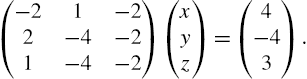
Solve the system  for x, y, and z.
Solution
In this case, entering either
Solve[{x-2y+z==-4,3x+2y-z==8,-x+3y+5z==0}]
or
Solve[{x-2y+z,3x+2y-z,-x+3y+5z}=={-4,8,0}]
give the same result.
![]()
![]()
![]()
Another way to solve systems of equations is based on the matrix form of the system of equations, ![]() . This system of equations is equivalent to the matrix equation
. This system of equations is equivalent to the matrix equation
The matrix of coefficients in the previous example is entered as matrixa along with the vector of right-hand side values vectorb. After defining the vector of variables, vectorx, the system ![]() is solved explicitly with the command Solve.
is solved explicitly with the command Solve.
![]()
![]()
![]()
![]()
![]()
![]()
![]() □
□
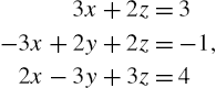
Example 5.16
Solve the system 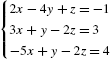 . Verify that the result returned satisfies the system.
Solution
To solve the system using Solve, we define eqs to be the set of three equations to be solved and vars to be the variables x, y, and z and then use Solve to solve the set of equations eqs for the variables in vars. The resulting output is named sols.
![]()
![]()
![]()
![]()
To verify that the result given in sols is the desired solution, we replace each occurrence of x, y, and z in eqs by the values found in sols using ReplaceAll (/.). Because the result indicates each of the three equations is satisfied, we conclude that the values given in sols are the components of the desired solution.
![]()
![]()
To solve the system using LinearSolve, we note that the system is equivalent to the matrix equation 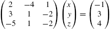 , define matrixa and vectorb, and use LinearSolve to solve this matrix equation.
![]()
![]()
![]()
![]()
To verify that the results are correct, we compute matrixa.solvector. Because the result is ![]() , we conclude that the solution to the system is
, we conclude that the solution to the system is 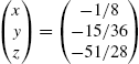 .
.
![]()
![]()
The command LinearSolve[A] returns a function that when given a vector b solves the equation ![]() : LinearSolve[A][b] returns x.
: LinearSolve[A][b] returns x.
![]()
![]() □
□
Enter indexed variables such ![]() ,
, ![]() , …,
, …, ![]() as x[1], x[2], …, x[n]. If you need to include the entire list, Table[x[i],{i,1,n}] usually produces the desired result(s).
as x[1], x[2], …, x[n]. If you need to include the entire list, Table[x[i],{i,1,n}] usually produces the desired result(s).
Example 5.17
Solve the system of equations 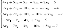 .
.
Solution
We solve the system in two ways. First, we use Solve to solve the system. Note that in this case, we enter the equations in the form
set of left-hand sides==set of right-hand sides.
![]()
![]()
![]()
![]()
![]()
![]()
We also use LinearSolve after defining matrixa and t2. As expected, in each case, the results are the same.
![]()
![]()
![]()
![]()
![]()
![]()
![]() □
□
5.2.2 Gauss–Jordan Elimination
Given the matrix equation ![]() , where
, where
the ![]() matrix A is called the coefficient matrix for the matrix equation
matrix A is called the coefficient matrix for the matrix equation ![]() and the
and the ![]() matrix
matrix

is called the augmented (or associated) matrix for the matrix equation. We may enter the augmented matrix associated with a linear system of equations directly or we can use commands like Join to help us construct the augmented matrix. For example, if A and B are rectangular matrices that have the same number of columns, Join[A,B] returns ![]() . On the other hand, if A and B are rectangular matrices that have the same number of rows, Join[A,B,2] returns the concatenated matrix
. On the other hand, if A and B are rectangular matrices that have the same number of rows, Join[A,B,2] returns the concatenated matrix ![]() .
.
Example 5.18
Solve the system 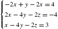 using Gauss–Jordan elimination.
Solution
The system is equivalent to the matrix equation
The augmented matrix associated with this system is
which we construct using the command Join.
![]()
![]()
![]()
![]()

We calculate the solution by row-reducing augm using RowReduce. Generally, RowReduce[A] reduces A to reduced row echelon form.
![]()
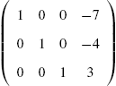
From this result, we see that the solution is
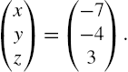
We verify this by replacing each occurrence of x, y, and z on the left-hand side of the equations by −7, −4, and 3, respectively, and noting that the components of the result are equal to the right-hand side of each equation.
![]()
![]()
![]() □
□
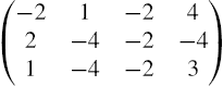
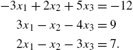
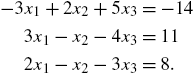
In the following example, we carry out the steps of the row reduction process.

Solution
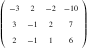
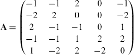
The augmented matrix is 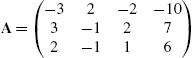 , defined in capa, and then displayed in traditional row-and-column form with MatrixForm. Given the matrix A, the ith part of A corresponds to the ith row of A. Therefore, A[[i]] returns the ith row of A.
![]()
![]()
![]()
We eliminate methodically. First, we multiply row 1 by ![]() so that the first entry in the first column is 1.
so that the first entry in the first column is 1.
![]()
![]()
We now eliminate below. First, we multiply row 1 by −3 and add it to row 2 and then we multiply row 1 by −2 and add it to row 3.
![]()
![]()
![]()
Observe that the first nonzero entry in the second row is 1. We eliminate below this entry by adding ![]() times row 2 to row 3.
times row 2 to row 3.
![]()
![]()
We multiply the third row by −3 so that the first nonzero entry is 1.
![]()
![]()
This matrix is equivalent to the system

which shows us that the solution is ![]() ,
, ![]() ,
, ![]() .
.
Working backwards confirms this. Multiplying row 2 by 2/3 and adding to row 1 and then multiplying row 3 by ![]() and adding to row 1 results in
and adding to row 1 results in
![]()
![]()
![]()
![]()
which is equivalent to the system ![]() ,
, ![]() ,
, ![]() .
.
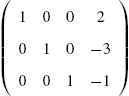
Equivalent results are obtained with RowReduce.
![]()
![]()
![]()
![]()
Finally, we confirm the result directly with Solve.
![]()
![]()
![]() □
□
It is important to remember that if you reduce the augmented matrix to reduced-row-echelon form, the results show you the solution to the problem. RowReduce[A] row reduces A to reduced-row-echelon form.
Solution
The augmented matrix is  , which is reduced to reduced row echelon form with RowReduce.
![]()
![]()
![]()
The result shows that the original system is equivalent to
so ![]() ,
, ![]() , or
, or ![]() is free. Choosing
is free. Choosing ![]() to be free, for any real number t, a solution to the system is
to be free, for any real number t, a solution to the system is
The system has infinitely many solutions.
Equivalent results are obtained with Solve.
![]()
![]()
![]() □
□
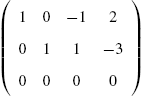
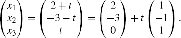
Example 5.21
Solution
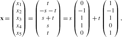
The augmented matrix is 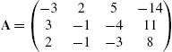 , which is reduced to reduced row echelon form with RowReduce.
![]()
![]()
![]()
![]()
The result shows that the original system is equivalent to

Of course, 0 is not equal to 1: the last equation is false. The system has no solutions.
We check the calculation with Solve. In this case, the results indicate that Solve cannot find any solutions to the system.
![]()
![]()
{}
Generally, if Mathematica returns nothing, the result means either that there is no solution or that Mathematica cannot solve the problem. Sometimes, Mathematica will return a warning message that solutions may exist but that it cannot find them. In these situations, we must always check using another method. □
Example 5.22
The nullspace of A is the set of solutions to the system of equations ![]() . Find the nullspace of
. Find the nullspace of  .
.
Solution
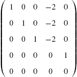
Observe that row reducing ![]() is equivalent to row reducing A. After defining A, we use RowReduce to row reduce A.
is equivalent to row reducing A. After defining A, we use RowReduce to row reduce A.
![]()
![]()
![]()
![]()
The result indicates that the solutions of ![]() are
are
where s and t are any real numbers. The dimension of the nullspace, the nullity, is 2; a basis for the nullspace is
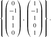
You can use the command NullSpace[A] to find a basis of the nullspace of a matrix A directly.
![]()
![]()
A is singular because ![]() .
.
![]()
0
Do not use LinearSolve on singular matrices:
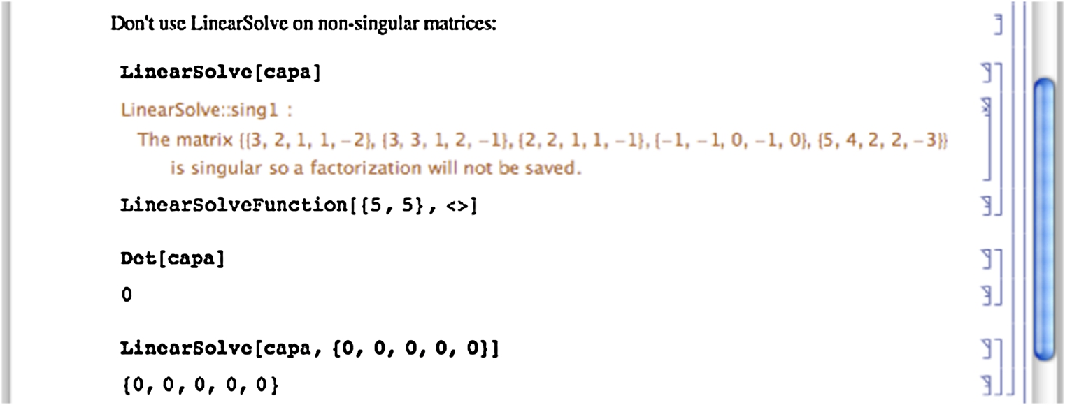
as the results returned may not be (completely) correct.
![]()
![]()
![]() □
□
5.3 Selected Topics from Linear Algebra
5.3.1 Fundamental Subspaces Associated with Matrices
Let ![]() be an
be an ![]() matrix with entry
matrix with entry ![]() in the ith row and jth column. The row space of A,
in the ith row and jth column. The row space of A, ![]() , is the spanning set of the rows of A; the column space of A,
, is the spanning set of the rows of A; the column space of A, ![]() , is the spanning set of the columns of A. If A is any matrix, then the dimension of the column space of A is equal to the dimension of the row space of A. The dimension of the row space (column space) of a matrix A is called the rank of A. The nullspace of A is the set of solutions to the system of equations
, is the spanning set of the columns of A. If A is any matrix, then the dimension of the column space of A is equal to the dimension of the row space of A. The dimension of the row space (column space) of a matrix A is called the rank of A. The nullspace of A is the set of solutions to the system of equations ![]() . The nullspace of A is a subspace and its dimension is called the nullity of A. The rank of A is equal to the number of nonzero rows in the row echelon form of A, the nullity of A is equal to the number of zero rows in the row echelon form of A. Thus, if A is a square matrix, the sum of the rank of A and the nullity of A is equal to the number of rows (columns) of A.
. The nullspace of A is a subspace and its dimension is called the nullity of A. The rank of A is equal to the number of nonzero rows in the row echelon form of A, the nullity of A is equal to the number of zero rows in the row echelon form of A. Thus, if A is a square matrix, the sum of the rank of A and the nullity of A is equal to the number of rows (columns) of A.
1. NullSpace[A] returns a list of vectors which form a basis for the nullspace (or kernel) of the matrix A.
2. RowReduce[A] yields the reduced row echelon form of the matrix A.
Example 5.23
Solution
We begin by defining the matrix matrixa. Then, RowReduce is used to place matrixa in reduced row echelon form.
![]()
![]()
![]()
![]()
Because the row-reduced form of matrixa contains four nonzero rows, the rank of A is 4 and thus the nullity is 1. We obtain a basis for the nullspace with NullSpace.
![]()
![]()
As expected, because the nullity is 1, a basis for the nullspace contains one vector. □
Example 5.24
Solution
A basis for the column space of B is the same as a basis for the row space of the transpose of B. We begin by defining matrixb and then using Transpose to compute the transpose of matrixb, naming the resulting output tb.
![]()
![]()
![]()
![]()
![]()
Next, we use RowReduce to row reduce tb and name the result rrtb. A basis for the column space consists of the first four elements of rrtb. We also use Transpose to show that the first four elements of rrtb are the same as the first four columns of the transpose of rrtb. Thus, the jth column of a matrix A can be extracted from A with Transpose [A][[j]].
![]()
![]()
We extract the first four elements of rrtb with Take. The results correspond to a basis for the column space of B.
![]()
![]() □
□
5.3.2 The Gram–Schmidt Process
A set of vectors ![]() is orthonormal means that
is orthonormal means that ![]() for all values of i and
for all values of i and ![]() for
for ![]() . Given a set of linearly independent vectors
. Given a set of linearly independent vectors ![]() , the set of all linear combinations of the elements of S,
, the set of all linear combinations of the elements of S, ![]() , is a vector space. Note that if S is an orthonormal set and
, is a vector space. Note that if S is an orthonormal set and ![]() , then
, then ![]() . Thus, we may easily express u as a linear combination of the vectors in S. Consequently, if we are given any vector space, V, it is frequently convenient to be able to find an orthonormal basis of V. We may use the Gram–Schmidt process to find an orthonormal basis of the vector space
. Thus, we may easily express u as a linear combination of the vectors in S. Consequently, if we are given any vector space, V, it is frequently convenient to be able to find an orthonormal basis of V. We may use the Gram–Schmidt process to find an orthonormal basis of the vector space ![]() .
.
We summarize the algorithm of the Gram–Schmidt process so that given a set of n linearly independent vectors ![]() , where
, where ![]() , we can construct a set of orthonormal vectors
, we can construct a set of orthonormal vectors ![]() so that
so that ![]() .
.
1. Let ![]() ;
;
2. Compute ![]() ,
, ![]() , and let
, and let
Then, ![]() and
and ![]() ;
;
3. Generally, for ![]() , compute
, compute
![]() , and let
, and let
Then, ![]() and
and
and
4. Because ![]() and
and ![]() is an orthonormal set,
is an orthonormal set, ![]() is an orthonormal basis of V.
is an orthonormal basis of V.
The Gram–Schmidt procedure is well-suited to computer arithmetic. The following code performs each step of the Gram–Schmidt process on a set of n linearly independent vectors ![]() . At the completion of each step of the procedure, gramschmidt[vecs] prints the list of vectors corresponding to
. At the completion of each step of the procedure, gramschmidt[vecs] prints the list of vectors corresponding to ![]() and returns the list of vectors
and returns the list of vectors ![]() . Note how comments are inserted into the code using (*...*).
. Note how comments are inserted into the code using (*...*).
![]()
![]()
![]()
![]()
![]()
![]()
![]()
![]()
![]()
![]()
![]()
![]()
![]()
![]()
![]()
![]()
![]()
Example 5.25
Use the Gram–Schmidt process to transform the basis  of
of ![]() into an orthonormal basis.
into an orthonormal basis.
Solution
We proceed by defining v1, v2, and v3 to be the vectors in the basis S and using gramschmidt[{v1,v2,v3}] to find an orthonormal basis.
![]()
![]()
![]()
![]()
![]()
![]()
![]()
On the first line of output, the result ![]() is given;
is given; ![]() appears on the second line;
appears on the second line; ![]() follows on the third. □
follows on the third. □
Example 5.26
Compute an orthonormal basis for the subspace of ![]() spanned by the vectors
spanned by the vectors ![]() ,
, ![]() , and
, and ![]() . Also, verify that the basis vectors are orthogonal and have norm 1.
. Also, verify that the basis vectors are orthogonal and have norm 1.
Solution
With gramschmidt, we compute the orthonormal basis vectors. Note that Mathematica names oset the last result returned by gramschmidt. The orthogonality of these vectors is then verified. Notice that Together is used to simplify the result in the case of oset[[2]].oset[[3]]. The norm of each vector is then found to be 1.
![]()
![]()
![]()
![]()
The three vectors are extracted with oset using oset[[1]], oset[[2]], and oset[[3]].
![]()
![]()
![]()
0
0
0
![]()
![]()
![]()
1
1
1 □
Mathematica contains functions that perform most of the operations discussed here.
1. Orthogonalize[{v1,v2,...},Method->GramSchmidt] returns an orthonormal set of vectors given the set of vectors ![]() . Note that this command does not illustrate each step of the Gram–Schmidt procedure as the gramschmidt function defined above.
. Note that this command does not illustrate each step of the Gram–Schmidt procedure as the gramschmidt function defined above.
2. Normalize[v] returns ![]() given the nonzero vector v.
given the nonzero vector v.
3. Projection[v1,v2] returns the projection of ![]() onto
onto ![]() :
: ![]() .
.
Thus,
![]()
![]()
returns an orthonormal basis for the subspace of ![]() spanned by the vectors
spanned by the vectors ![]() ,
, ![]() , and
, and ![]() . The command
. The command
![]()
![]()
finds a unit vector with the same direction as the vector  . Entering
![]()
![]()
finds the projection of onto  .
.
5.3.3 Linear Transformations
A function ![]() is a linear transformation means that T satisfies the properties
is a linear transformation means that T satisfies the properties ![]() and
and ![]() for all vectors u and v in
for all vectors u and v in ![]() and all real numbers c. Let
and all real numbers c. Let ![]() be a linear transformation and suppose
be a linear transformation and suppose ![]() ,
, ![]() , …,
, …, ![]() where
where ![]() represents the standard basis of
represents the standard basis of ![]() and
and ![]() ,
, ![]() , …,
, …, ![]() are (column) vectors in
are (column) vectors in ![]() . The associated matrix of T is the
. The associated matrix of T is the ![]() matrix
matrix ![]() :
:
Moreover, if A is any ![]() matrix, then A is the associated matrix of the linear transformation defined by
matrix, then A is the associated matrix of the linear transformation defined by ![]() . In fact, a linear transformation T is completely determined by its action on any basis.
. In fact, a linear transformation T is completely determined by its action on any basis.
The kernel of the linear transformation T, ![]() , is the set of all vectors x in
, is the set of all vectors x in ![]() such that
such that ![]() :
: ![]() . The kernel of T is a subspace of
. The kernel of T is a subspace of ![]() . Because
. Because ![]() for all x in
for all x in ![]() ,
, ![]() so the kernel of T is the same as the nullspace of A.
so the kernel of T is the same as the nullspace of A.
Example 5.27
Let ![]() be the linear transformation defined by
be the linear transformation defined by  . (a) Calculate a basis for the kernel of the linear transformation. (b) Determine which of the vectors
 ![]() and
and ![]() is in the kernel of T.
is in the kernel of T.
Solution
We begin by defining matrixa to be the matrix  and then defining t. A basis for the kernel of T is the same as a basis for the nullspace of A found with NullSpace.
![]()
![]()
![]()
![]()
![]()
![]()
Because ![]() is a linear combination of the vectors that form a basis for the kernel,
is a linear combination of the vectors that form a basis for the kernel, ![]() is in the kernel while
is in the kernel while ![]() is not. These results are verified by evaluating t for each vector.
is not. These results are verified by evaluating t for each vector.
![]()
![]()
![]()
![]() □
□
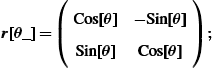
Application: Rotations
Let ![]() be a vector in
be a vector in ![]() and θ an angle. Then, there are numbers r and ϕ given by
and θ an angle. Then, there are numbers r and ϕ given by ![]() and
and ![]() so that
so that ![]() and
and ![]() . When we rotate
. When we rotate ![]() through the angle θ, we obtain the vector
through the angle θ, we obtain the vector ![]() . Using the trigonometric identities
. Using the trigonometric identities ![]() and
and ![]() we rewrite
we rewrite
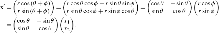
Thus, the vector ![]() is obtained from x by computing
is obtained from x by computing ![]() . Generally, if θ represents an angle, the linear transformation
. Generally, if θ represents an angle, the linear transformation ![]() defined by
defined by ![]() is called the rotation of
is called the rotation of ![]() through the angle θ. We write code to rotate a polygon through an angle θ. The procedure rotate uses a list of n points and the rotation matrix defined in r to produce a new list of points that are joined using the Line graphics directive. Entering
through the angle θ. We write code to rotate a polygon through an angle θ. The procedure rotate uses a list of n points and the rotation matrix defined in r to produce a new list of points that are joined using the Line graphics directive. Entering
Line[{{x1,y1},{x2,y2},...,{xn,yn}}]
represents the graphics primitive for a line in two dimensions that connects the points listed in {{x1,y1},{x2,y2},...,{xn,yn}}. Entering
Show[Graphics[Line[{{x1,y1},{x2,y2},...,{xn,yn}}]]]
displays the line. This rotation can be determined for one value of θ. However, a more interesting result is obtained by creating a list of rotations for a sequence of angles and then displaying the graphics objects. This is done for ![]() to
to ![]() using increments of
using increments of ![]() . Hence, a list of nine graphs is given for the square with vertices
. Hence, a list of nine graphs is given for the square with vertices ![]() ,
, ![]() ,
, ![]() , and
, and ![]() and displayed in Fig. 5.7.
and displayed in Fig. 5.7.

![]()
![]()
![]()
![]()
![]()
![]()
![]()
![]()
![]()
![]()
![]()
5.3.4 Eigenvalues and Eigenvectors
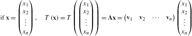
Let A be an ![]() matrix. λ is an eigenvalue of A if there is a nonzero vector, v, called an eigenvector, satisfying
matrix. λ is an eigenvalue of A if there is a nonzero vector, v, called an eigenvector, satisfying ![]() . Because
. Because ![]() has a unique solution of
has a unique solution of ![]() if
if ![]() , to find non-zero solutions, v, of
, to find non-zero solutions, v, of ![]() , we begin by solving
, we begin by solving ![]() . That is, we find the eigenvalues of A by solving the characteristic polynomial
. That is, we find the eigenvalues of A by solving the characteristic polynomial ![]() for λ. Once we find the eigenvalues, the corresponding eigenvectors are found by solving
for λ. Once we find the eigenvalues, the corresponding eigenvectors are found by solving ![]() for v.
for v.
If A is ![]() , Eigenvalues[A] finds the eigenvalues of A, Eigenvectors[A] finds the eigenvectors, and Eigensystem[A] finds the eigenvalues and corresponding eigenvectors. CharacteristicPolynomial[A,lambda] finds the characteristic polynomial of A as a function of λ.
, Eigenvalues[A] finds the eigenvalues of A, Eigenvectors[A] finds the eigenvectors, and Eigensystem[A] finds the eigenvalues and corresponding eigenvectors. CharacteristicPolynomial[A,lambda] finds the characteristic polynomial of A as a function of λ.
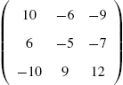
Example 5.28
Find the eigenvalues and corresponding eigenvectors for each of the following matrices. (a) ![]() , (b)
, (b) ![]() , (c)
, (c)  , and (d)
 ![]() .
.
Solution
(a) We begin by finding the eigenvalues. Solving

gives us ![]() and
and ![]() .
.
Observe that the same results are obtained using CharacteristicPolynomial and Eigenvalues.
![]()
![]()
![]()
![]()
![]()
![]()
![]()
We now find the corresponding eigenvectors. Let ![]() be an eigenvector corresponding to
be an eigenvector corresponding to ![]() , then
, then
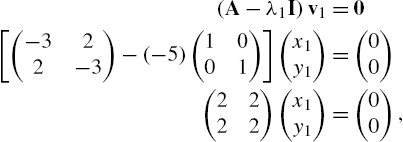
which row reduces to
That is, ![]() or
or ![]() . Hence, for any value of
. Hence, for any value of ![]() ,
,
is an eigenvector corresponding to ![]() . Of course, this represents infinitely many vectors. But, they are all linearly dependent. Choosing
. Of course, this represents infinitely many vectors. But, they are all linearly dependent. Choosing ![]() yields
yields ![]() . Note that you might have chosen
. Note that you might have chosen ![]() and obtained
and obtained ![]() . However, both of our results are “correct” because these vectors are linearly dependent.
. However, both of our results are “correct” because these vectors are linearly dependent.
Similarly, letting ![]() be an eigenvector corresponding to
be an eigenvector corresponding to ![]() we solve
we solve ![]() :
:

Thus, ![]() or
or ![]() . Hence, for any value of
. Hence, for any value of ![]() ,
,

is an eigenvector corresponding to ![]() . Choosing
. Choosing ![]() yields
yields ![]() . We confirm these results using RowReduce.
. We confirm these results using RowReduce.
![]()
![]()
![]()
![]()
![]()
We obtain the same results using Eigenvectors and Eigensystem.
![]()
![]()
![]()
![]()
(b) In this case, we see that ![]() has multiplicity 2. There is only one linearly independent eigenvector,
has multiplicity 2. There is only one linearly independent eigenvector, ![]() , corresponding to λ.
, corresponding to λ.
![]()
![]()
![]()
![]()
![]()
![]()
![]()
(c) The eigenvalue ![]() has corresponding eigenvector
has corresponding eigenvector  . The eigenvalue
 ![]() has multiplicity 2. In this case, there are two linearly independent eigenvectors corresponding to this eigenvalue:
has multiplicity 2. In this case, there are two linearly independent eigenvectors corresponding to this eigenvalue:  and
and  .
.
![]()
![]()
![]()
![]()
![]()
![]()
![]()
(d) In this case, the eigenvalues ![]() are complex conjugates. We see that the eigenvectors
are complex conjugates. We see that the eigenvectors ![]() are complex conjugates as well.
are complex conjugates as well.
![]()
![]()
![]()
![]()
![]()
![]()
![]()
![]()
![]()
![]() □
□
5.3.5 Jordan Canonical Form
Let ![]() represent a
represent a ![]() matrix with the indicated elements. The
matrix with the indicated elements. The ![]() Jordan block matrix is given by
Jordan block matrix is given by ![]() where λ is a constant:
where λ is a constant:
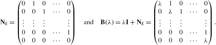
Hence, ![]() can be defined as
can be defined as  . A Jordan matrix has the form
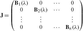
where the entries ![]() ,
, ![]() , 2, …, n represent Jordan block matrices.
, 2, …, n represent Jordan block matrices.
Suppose that A is an ![]() matrix. Then there is an invertible
matrix. Then there is an invertible ![]() matrix C such that
matrix C such that ![]() where J is a Jordan matrix with the eigenvalues of A as diagonal elements. The matrix J is called the Jordan canonical form of A. The command
where J is a Jordan matrix with the eigenvalues of A as diagonal elements. The matrix J is called the Jordan canonical form of A. The command
JordanDecomposition[m]
yields a list of matrices {s,j} such that m=s.j.Inverse[s] and j is the Jordan canonical form of the matrix m.
For a given matrix A, the unique monic polynomial q of least degree satisfying ![]() is called the minimal polynomial of A. Let p denote the characteristic polynomial of A. Because
is called the minimal polynomial of A. Let p denote the characteristic polynomial of A. Because ![]() , it follows that q divides p. We can use the Jordan canonical form of a matrix to determine its minimal polynomial.
, it follows that q divides p. We can use the Jordan canonical form of a matrix to determine its minimal polynomial.
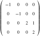
Example 5.29
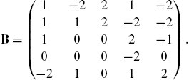
Find the Jordan canonical form, ![]() , of
, of 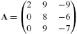 .
.
Solution
After defining matrixa, we use JordanDecomposition to find the Jordan canonical form of a and name the resulting output ja.
![]()
![]()
![]()
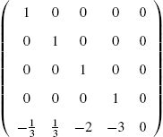
The Jordan matrix corresponds to the second element of ja extracted with ja[[2]] and displayed in MatrixForm.
![]()
We also verify that the matrices ja[[1]] and ja[[2]] satisfy
matrixa=ja[[1]].ja[[2]].Inverse[ja[[1]]].
![]()
![]()
Next, we use CharacteristicPolynomial to find the characteristic polynomial of matrixa and then verify that matrixa satisfies its characteristic polynomial.
![]()
![]()
![]()
![]()
From the Jordan form, we see that the minimal polynomial of A is ![]() . We define the minimal polynomial to be q and then verify that matrixa satisfies its minimal polynomial.
. We define the minimal polynomial to be q and then verify that matrixa satisfies its minimal polynomial.
![]()
![]()
![]()
![]()
As expected, q divides p.
![]()
![]() □
□
Example 5.30
If  , find the characteristic and minimal polynomials of A.
Solution
As in the previous example, we first define matrixa and then use JordanDecomposition to find the Jordan canonical form of A.
![]()
![]()
![]()
![]()
The Jordan canonical form of A is the second element of ja, extracted with ja[[2]] and displayed in MatrixForm.
![]()
From this result, we see that the minimal polynomial of A is ![]() . We define q to be the minimal polynomial of A and then verify that matrixa satisfies q.
. We define q to be the minimal polynomial of A and then verify that matrixa satisfies q.
![]()
![]()
![]()
![]()
The characteristic polynomial is obtained next and named p. As expected, q divides p, verified with Cancel.
![]()
![]()
![]()
![]() □
□
5.3.6 The QR Method
The conjugate transpose (or Hermitian adjoint matrix) of the ![]() complex matrix A which is denoted by
complex matrix A which is denoted by ![]() is the transpose of the complex conjugate of A. Symbolically, we have
is the transpose of the complex conjugate of A. Symbolically, we have ![]() . A complex matrix A is unitary if
. A complex matrix A is unitary if ![]() . Given a matrix A, there is a unitary matrix Q and an upper triangular matrix R such that
. Given a matrix A, there is a unitary matrix Q and an upper triangular matrix R such that ![]() . The product matrix QR is called the QR factorization of A. The command
. The product matrix QR is called the QR factorization of A. The command
QRDecomposition[N[m]]
determines the QR decomposition of the matrix m by returning the list {q,r}, where q is an orthogonal matrix, r is an upper triangular matrix and m=Transpose[q].r.
Example 5.31
Find the QR factorization of the matrix  .
.
Solution
We define matrixa and then use QRDecomposition to find the QR decomposition of matrixa, naming the resulting output qrm.
![]()
![]()
![]()
The first matrix in qrm is extracted with qrm[[1]] and the second with qrm[[2]].
![]()
![]()
We verify that the results returned are the QR decomposition of A.
![]()
 □
□
One of the most efficient and most widely used methods for numerically calculating the eigenvalues of a matrix is the QR Method. Given a matrix A, then there is a Hermitian matrix Q and an upper triangular matrix R such that ![]() . If we define a sequence of matrices
. If we define a sequence of matrices ![]() , factored as
, factored as ![]() ;
; ![]() , factored as
, factored as ![]() ;
; ![]() , factored as
, factored as ![]() ; and in general,
; and in general, ![]() ,
, ![]() , 2, … then the sequence
, 2, … then the sequence ![]() converges to a triangular matrix with the eigenvalues of A along the diagonal or to a nearly triangular matrix from which the eigenvalues of A can be calculated rather easily.
converges to a triangular matrix with the eigenvalues of A along the diagonal or to a nearly triangular matrix from which the eigenvalues of A can be calculated rather easily.
Example 5.32
Consider the ![]() matrix
matrix  . Approximate the eigenvalues of A with the QR Method.
Solution
We define the sequence a and qr recursively. We define a using the form a[n_]:=a[n]=... and qr using the form qr[n_]:=qr[n]=... so that Mathematica “remembers” the values of a and qr computed, and thus Mathematica avoids recomputing values previously computed. This is of particular advantage when computing a[n] and qr[n] for large values of n.
![]()
![]()
![]()
![]()
![]()
We illustrate a[n] and qr[n] by computing qr[9] and a[10]. Note that computing a[10] requires the computation of qr[9]. From the results, we suspect that the eigenvalues of A are 5 and 2.
![]()
![]()
![]()
Next, we compute a[n] for ![]() , 10, and 15, displaying the result in TableForm. We obtain further evidence that the eigenvalues of A are 5 and 2.
, 10, and 15, displaying the result in TableForm. We obtain further evidence that the eigenvalues of A are 5 and 2.
![]()
We verify that the eigenvalues of A are indeed 5 and 2 with Eigenvalues.
![]()
![]() □
□
5.4 Maxima and Minima Using Linear Programming
5.4.1 The Standard Form of a Linear Programming Problem
We call the linear programming problem of the following form the standard form of the linear programming problem:
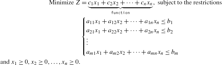
The command
Minimize[{function,inequalities},{variables}]
solves the standard form of the linear programming problem. Similarly, the command
Maximize[{function,inequalities},{variables}]
solves the linear programming problem: Maximize ![]() , subject to the restrictions
, subject to the restrictions
and ![]() ,
, ![]() , …,
, …, ![]() .
.
Example 5.33
Maximize ![]() subject to the constraints
subject to the constraints ![]() ,
, ![]() ,
, ![]() , and
, and ![]() ,
, ![]() ,
, ![]() all nonnegative.
all nonnegative.
Solution
In order to solve a linear programming problem with Mathematica, the variables {x1,x2,x3} and objective function z[x1,x2,x3] are first defined. In an effort to limit the amount of typing required to complete the problem, the set of inequalities is assigned the name ineqs while the set of variables is called vars. The symbol “<=”, obtained by typing the “<” key and then the “=” key, represents “less than or equal to” and is used in ineqs. Hence, the maximization problem is solved with the command
Maximize[{z[x1,x2,x3],ineqs},vars].
![]()
![]()
![]()
![]()
![]()
![]()
![]()
The solution gives the maximum value of z subject to the given constraints as well as the values of x1, x2, and x3 that maximize z. Thus, we see that the maximum value of Z is 45 if ![]() ,
, ![]() , and
, and ![]() . □
. □
We demonstrate the use of Minimize in the following example.
Example 5.34
Minimize ![]() subject to the constraints
subject to the constraints ![]() ,
, ![]() ,
, ![]() , and x, y, z all nonnegative.
, and x, y, z all nonnegative.
Solution
After clearing all previously used names of functions and variable values, the variables, objective function, and set of constraints for this problem are defined and entered as they were in the first example. By using Minimize, the minimum value of the objective function is obtained as well as the variable values that give this minimum.
![]()
![]()
![]()
![]()
![]()
![]()
![]()
We conclude that the minimum value is −90 and occurs if ![]() ,
, ![]() , and
, and ![]() . □
. □
5.4.2 The Dual Problem
Given the standard form of the linear programming problem in equations (5.2), the dual problem is as follows: “Maximize ![]() subject to the constraints
subject to the constraints ![]() for
for ![]() , 2, …, n and
, 2, …, n and ![]() for
for ![]() , 2, …, m.” Similarly, for the problem: “Maximize
, 2, …, m.” Similarly, for the problem: “Maximize ![]() subject to the constraints
subject to the constraints ![]() for
for ![]() , 2, …, m and
, 2, …, m and ![]() for
for ![]() , 2, …, n,” the dual problem is as follows: “Minimize
, 2, …, n,” the dual problem is as follows: “Minimize ![]() subject to the constraints
subject to the constraints ![]() for
for ![]() , 2, …, n and
, 2, …, n and ![]() for
for ![]() , 2, …, m.”
, 2, …, m.”
Example 5.35
Maximize ![]() subject to the constraints
subject to the constraints ![]() ,
, ![]() ,
, ![]() , and
, and ![]() . State the dual problem and find its solution.
. State the dual problem and find its solution.
Solution
First, the original (or primal) problem is solved. The objective function for this problem is represented by zx. Finally, the set of inequalities for the primal is defined to be ineqsx. Using the command
Maximize[{zx,ineqsx},{x[1],x[2]}],
the maximum value of zx is found to be 45.
![]()
![]()
![]()
![]()
![]()
Because in this problem we have ![]() ,
, ![]() ,
, ![]() , and
, and ![]() , the dual problem is as follows: Minimize
, the dual problem is as follows: Minimize ![]() subject to the constraints
subject to the constraints ![]() ,
, ![]() ,
, ![]() , and
, and ![]() . The dual is solved in a similar fashion by defining the objective function zy and the collection of inequalities ineqsy. The minimum value obtained by zy subject to the constraints ineqsy is 45, which agrees with the result of the primal and is found with
. The dual is solved in a similar fashion by defining the objective function zy and the collection of inequalities ineqsy. The minimum value obtained by zy subject to the constraints ineqsy is 45, which agrees with the result of the primal and is found with
Minimize[{zy,ineqsy},{y[1],y[2]}].
![]()
![]()
![]()
![]() □
□
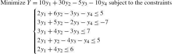
Of course, linear programming models can involve numerous variables. Consider the following: given the standard form linear programming problem in equations (5.2), let  ,
,  ,
, ![]() , and A denote the
, and A denote the ![]() matrix
matrix  . Then the standard form of the linear programming problem is equivalent to finding the vector x that maximizes
 ![]() subject to the restrictions
subject to the restrictions ![]() and
and ![]() ,
, ![]() , …,
, …, ![]() . The dual problem is: “Minimize
. The dual problem is: “Minimize ![]() where
where ![]() subject to the restrictions
subject to the restrictions ![]() (componentwise) and
(componentwise) and ![]() ,
, ![]() , …,
, …, ![]() .”
.”
The command
LinearProgramming[c,A,b]
finds the vector x that minimizes the quantity Z=c.x subject to the restrictions A.x>=b and x>=0. LinearProgramming does not yield the minimum value of Z as did Minimize and Maximize and the value must be determined from the resulting vector.
Example 5.36
Maximize ![]() subject to the constraints
subject to the constraints ![]() ,
, ![]() ,
, ![]() ,
, ![]() , and
, and ![]() for
for ![]() , 2, 3, 4, and 5. State the dual problem. What is its solution?
, 2, 3, 4, and 5. State the dual problem. What is its solution?
Solution
For this problem,  ,
,  ,
, ![]() , and
, and  . First, the vectors c and b are entered and then matrix A is entered and named matrixa.
![]()
![]()
![]()
![]()
Next, we use Array[x,5] to create the list of five elements {x[1],x[2],...,x[5]} named xvec. The command Table[x[i], {i,1,5}] returns the same list. These variables must be defined before attempting to solve this linear programming problem.
![]()
![]()
After entering the objective function coefficients with the vector c, the matrix of coefficients from the inequalities with matrixa, and the right-hand side values found in b; the problem is solved with
LinearProgramming[c,matrixa,b].
The solution is called xvec. Hence, the maximum value of the objective function is obtained by evaluating the objective function at the variable values that yield a maximum. Because these values are found in xvec, the maximum is determined with the dot product of the vector c and the vector xvec. (Recall that this product is entered as c.xvec.) This value is found to be 35/4.
![]()
![]()
![]()
![]()
Because the dual of the problem is “Minimize the number Y=y.b subject to the restrictions y.A<c and y>0,” we use Mathematica to calculate y.b and y.A. A list of the dual variables {y[1],y[2],y[3],y[4]} is created with Array[y,4]. This list includes four elements because there are four constraints in the original problem. The objective function of the dual problem is, therefore, found with yvec.b, and the left-hand sides of the set of inequalities are given with yvec.matrixa.
![]()
![]()
![]()
![]()
![]()
![]()
Hence, we may state the dual problem as:
and ![]() for
for ![]() , 2, 3, and 4. □
, 2, 3, and 4. □
Application: A Transportation Problem
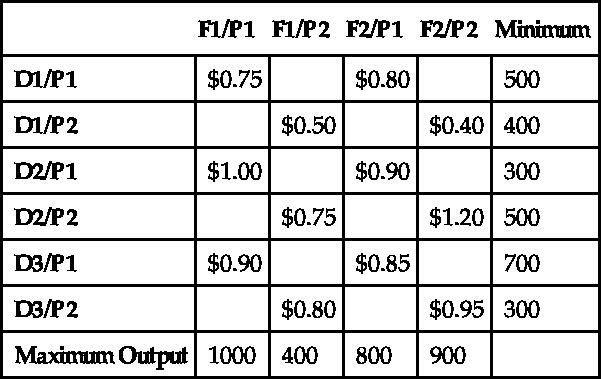
A certain company has two factories, F1 and F2, each producing two products, P1 and P2, that are to be shipped to three distribution centers, D1, D2, and D3. The following table illustrates the cost associated with shipping each product from the factory to the distribution center, the minimum number of each product each distribution center needs, and the maximum output of each factory. How much of each product should be shipped from each plant to each distribution center to minimize the total shipping costs?
| F1/P1 | F1/P2 | F2/P1 | F2/P2 | Minimum | |
| D1/P1 | $0.75 | $0.80 | 500 | ||
| D1/P2 | $0.50 | $0.40 | 400 | ||
| D2/P1 | $1.00 | $0.90 | 300 | ||
| D2/P2 | $0.75 | $1.20 | 500 | ||
| D3/P1 | $0.90 | $0.85 | 700 | ||
| D3/P2 | $0.80 | $0.95 | 300 | ||
| Maximum Output | 1000 | 400 | 800 | 900 |
Solution
Let ![]() denote the number of units of P1 shipped from F1 to D1;
denote the number of units of P1 shipped from F1 to D1; ![]() the number of units of P2 shipped from F1 to D1;
the number of units of P2 shipped from F1 to D1; ![]() the number of units of P1 shipped from F1 to D2;
the number of units of P1 shipped from F1 to D2; ![]() the number of units of P2 shipped from F1 to D2;
the number of units of P2 shipped from F1 to D2; ![]() the number of units of P1 shipped from F1 to D3;
the number of units of P1 shipped from F1 to D3; ![]() the number of units of P2 shipped from F1 to D3;
the number of units of P2 shipped from F1 to D3; ![]() the number of units of P1 shipped from F2 to D1;
the number of units of P1 shipped from F2 to D1; ![]() the number of units of P2 shipped from F2 to D1;
the number of units of P2 shipped from F2 to D1; ![]() the number of units of P1 shipped from F2 to D2;
the number of units of P1 shipped from F2 to D2; ![]() the number of units of P2 shipped from F2 to D2;
the number of units of P2 shipped from F2 to D2; ![]() the number of units of P1 shipped from F2 to D3; and
the number of units of P1 shipped from F2 to D3; and ![]() the number of units of P2 shipped from F2 to D3.
the number of units of P2 shipped from F2 to D3.
Then, it is necessary to minimize the number
subject to the constraints ![]() ,
, ![]() ,
, ![]() ,
, ![]() ,
, ![]() ,
, ![]() ,
, ![]() ,
, ![]() ,
, ![]() ,
, ![]() , and
, and ![]() nonnegative for
nonnegative for ![]() , 2, …, 12. In order to solve this linear programming problem, the objective function which computes the total cost, the 12 variables, and the set of inequalities must be entered. The coefficients of the objective function are given in the vector c. Using the command Array[x,12] illustrated in the previous example to define the list of 12 variables {x[1],x[2],...,x[12]}, the objective function is given by the product z=xvec.c, where xvec is the name assigned to the list of variables.
, 2, …, 12. In order to solve this linear programming problem, the objective function which computes the total cost, the 12 variables, and the set of inequalities must be entered. The coefficients of the objective function are given in the vector c. Using the command Array[x,12] illustrated in the previous example to define the list of 12 variables {x[1],x[2],...,x[12]}, the objective function is given by the product z=xvec.c, where xvec is the name assigned to the list of variables.
![]()
![]()
![]()
![]()
![]()
![]()
![]()
![]()
![]()
![]()
![]()
The set of constraints are then entered and named constraints for easier use. Therefore, the minimum cost and the value of each variable which yields this minimum cost are found with the command
Minimize[{z,constraints},xvec].
![]()
![]()
![]()
![]()
![]()
![]()
![]()
![]()
![]()
![]()
![]()
![]()
Notice that values is a list consisting of two elements: the minimum value of the cost function, 2115, and the list of the variable values {x[1]->500,x[2]->0, ...}. Hence, the minimum cost is obtained with the command values[[1]] and the list of variable values that yield the minimum cost is extracted with values[[2]].
![]()
2115.
![]()
![]()
Using these extraction techniques, the number of units produced by each factory can be computed. Because ![]() denotes the number of units of P1 shipped from F1 to D1,
denotes the number of units of P1 shipped from F1 to D1, ![]() the number of units of P1 shipped from F1 to D2, and
the number of units of P1 shipped from F1 to D2, and ![]() the number of units of P1 shipped from F1 to D3, the total number of units of Product 1 produced by Factory 1 is given by the command x[1]+x[3]+x[5] /. values[[2]] which evaluates this sum at the values of x[1], x[3], and x[5] given in the list values[[2]].
the number of units of P1 shipped from F1 to D3, the total number of units of Product 1 produced by Factory 1 is given by the command x[1]+x[3]+x[5] /. values[[2]] which evaluates this sum at the values of x[1], x[3], and x[5] given in the list values[[2]].
![]()
700.
Also, the number of units of Products 1 and 2 received by each distribution center can be computed. The command x[3]+x[9] //values[[2]] gives the total amount of P1 received at D2 because x[3]=amount of P1 received by D2 from F1 and x[9]= amount of P1 received by D2 from F2. Notice that this amount is the minimum number of units (300) of P1 requested by D2.
![]()
300.
The number of units of each product that each factory produces can be calculated and the amount of P1 and P2 received at each distribution center is calculated in a similar manner.
![]()
![]()
![]()
![]()
TableForm
![]()
From these results, we see that F1 produces 700 units of P1, F1 produces 400 units of P2, F2 produces 800 units of P1, F2 produces 800 units of P2, and each distribution center receives exactly the minimum number of each product it requests. □
5.5 Selected Topics from Vector Calculus
5.5.1 Vector-Valued Functions
We now turn our attention to vector-valued functions. In particular, we consider vector-valued functions of the following forms.
For the vector-valued functions (5.3) and (5.4), differentiation and integration are carried out term-by-term, provided that all the terms are differentiable and integrable. Suppose that C is a smooth curve defined by ![]() ,
, ![]() .
.
1. If ![]() , the unit tangent vector,
, the unit tangent vector, ![]() , is
, is ![]() .
.
2. If ![]() , the principal unit normal vector,
, the principal unit normal vector, ![]() , is
, is ![]() .
.
3. The arc length function, ![]() , is
, is ![]() . In particular, the length of C on the interval
. In particular, the length of C on the interval ![]() is
is ![]() .
.
4. The curvature, κ, of C is
where ![]() and
and ![]() .
.
It is a good exercise to show that the curvature of a circle of radius r is ![]() .
.
In 2-space, ![]() and
and ![]() . In 3-space
. In 3-space ![]() ,
, ![]() , and
, and ![]() .
.
Example 5.37
Folium of Descartes
Solution
(a) After defining ![]() ,
,
![]()
![]()
we compute ![]() and
and ![]() with ′, ″ and Integrate, respectively. We name
with ′, ″ and Integrate, respectively. We name ![]() dr,
dr, ![]() dr2, and
dr2, and ![]() ir.
ir.
![]()
![]()
![]()
![]()
![]()
![]()
(b) Mathematica does not automatically make assumptions regarding the value of t, so it does not algebraically simplify ![]() as we might typically do unless we use PowerExpand
as we might typically do unless we use PowerExpand
PowerExpand[Sqrt[x̂2]] returns x rather than ![]() .
.
![]()
![]()
The unit tangent vector, ![]() is formed in ut.
is formed in ut.
![]()
![]()
We perform the same steps to compute the unit normal vector, ![]() . In particular, note that
. In particular, note that ![]() .
.
![]()
![]()
![]()
![]()
![]()
![]()
![]()
![]()
(c) We use the formula ![]() to determine the curvature in curvature.
to determine the curvature in curvature.
![]()
![]()
We graphically illustrate the unit tangent and normal vectors at ![]() . First, we compute the unit tangent and normal vectors if
. First, we compute the unit tangent and normal vectors if ![]() using /. (ReplaceAll).
using /. (ReplaceAll).
![]()
![]()
![]()
![]()
We then compute the curvature if ![]() in smallk. The center of the osculating circle at
in smallk. The center of the osculating circle at ![]() is found in x0 and y0.
is found in x0 and y0.
The radius of the osculating circle is ![]() ; the position vector of the center is
; the position vector of the center is ![]() .
.
![]()
![]()
![]()
![]()
![]()
3.77124
![]()
![]()
We now graph ![]() with ParametricPlot. The unit tangent and normal vectors at
with ParametricPlot. The unit tangent and normal vectors at ![]() are graphed with Arrow in a1 and a2. The osculating circle at
are graphed with Arrow in a1 and a2. The osculating circle at ![]() is graphed with Circle in c1. All four graphs are displayed together with Show in Fig. 5.8.
is graphed with Circle in c1. All four graphs are displayed together with Show in Fig. 5.8.
Graphics[Circle[{x0, y0}, r]] is a two-dimensional graphics object that represents a circle of radius r centered at the point ![]() . Use Show to display the graph.
. Use Show to display the graph.
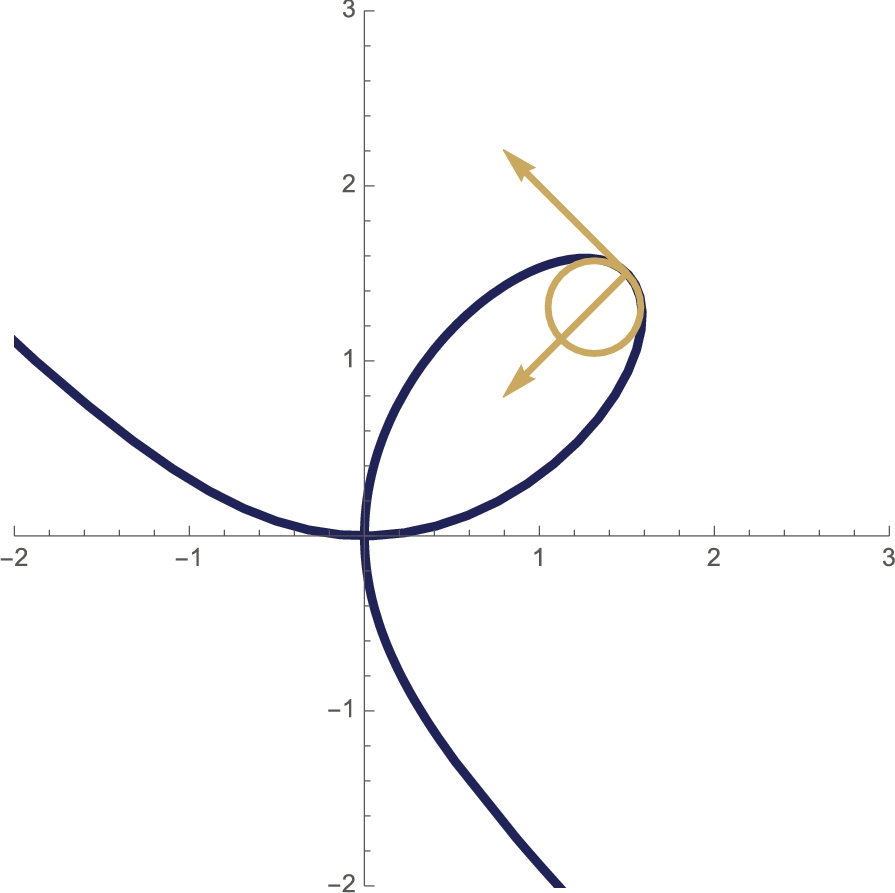
![]()
![]()
![]()
![]()
![]()
![]()
![]()
(d) The loop is formed by graphing ![]() for
for ![]() . Hence, the length of the loop is given by the improper integral
. Hence, the length of the loop is given by the improper integral ![]() , which we compute with NIntegrate.
, which we compute with NIntegrate.
![]()
4.91749 □
In the example, we computed the curvature at ![]() . Of course, we could choose other t values. With Manipulate,
. Of course, we could choose other t values. With Manipulate,
![]()
![]()
![]()
![]()
![]()
![]()
![]()
![]()
![]()
![]()
![]()
![]()
![]()
![]()
![]()
![]()
![]()
![]()
![]()
![]()
![]()
![]()
![]()
we can see the osculating circle at various values of ![]() . See Fig. 5.9.
. See Fig. 5.9.
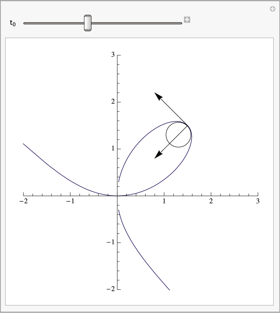
Of course, this particular choice of using the folium to illustrate the procedure could be modified as well. With
![]()
![]()
![]()
![]()
![]()
![]()
![]()
![]()
![]()
![]()
![]()
![]()
![]()
![]()
![]()
![]()
![]()
![]()
![]()
![]()
![]()
![]()
![]()
![]()
![]()
![]()
![]()
![]()
![]()
![]()
we not only allow ![]() to vary but also
to vary but also ![]() . Note that the resulting Manipulate object is quite slow on all except the fastest computers. See Fig. 5.10 (b).
. Note that the resulting Manipulate object is quite slow on all except the fastest computers. See Fig. 5.10 (b).

Recall that the gradient of ![]() is the vector-valued function
is the vector-valued function ![]() . Similarly, we define the gradient of
. Similarly, we define the gradient of ![]() to be
to be

A vector field F is conservative if there is a function f, called a potential function, satisfying ![]() . In the special case that
. In the special case that ![]() , F is conservative if and only if
, F is conservative if and only if
The divergence of the vector field ![]() is the scalar field
is the scalar field
The Div command can be used to find the divergence of a vector field:
Div[{P(x,y,z),Q(x,y,z),R(x,y,z)},"Cartesian"]
computes the divergence of ![]() in the Cartesian coordinate system. If you omit “Cartesian,” the default coordinates are the Cartesian coordinate system. However, if you are using a non-Cartesian coordinates system such as cylindrical or spherical coordinates, be sure to replace “Cartesian” with “Cylindrical,” “Spherical” or the name of the coordinate system you are using. Note that Mathematica supports nearly all coordinate systems used by scientists.
in the Cartesian coordinate system. If you omit “Cartesian,” the default coordinates are the Cartesian coordinate system. However, if you are using a non-Cartesian coordinates system such as cylindrical or spherical coordinates, be sure to replace “Cartesian” with “Cylindrical,” “Spherical” or the name of the coordinate system you are using. Note that Mathematica supports nearly all coordinate systems used by scientists.
The Laplacian of the scalar field ![]() is defined to be
is defined to be
In the same way that Div computes the divergence of a vector field Laplacian computes the Laplacian of a scalar field.
The curl of the vector field ![]() is
is

If ![]() , F is conservative if and only if
, F is conservative if and only if ![]() , in which case F is said to be irrotational.
, in which case F is said to be irrotational.
Example 5.38
Solution
We define ![]() and
and ![]()
![]() . Then we use D and Simplify to see that
. Then we use D and Simplify to see that ![]() . Hence, F is conservative.
. Hence, F is conservative.
![]()
![]()
![]()
![]()
![]()
![]()
We use Integrate to find f satisfying ![]() .
.
![]()
![]()
![]()
![]()
Therefore, ![]() , where C is an arbitrary constant. Letting
, where C is an arbitrary constant. Letting ![]() gives us the following potential function.
gives us the following potential function.
![]()
![]()
Remember that the vectors F are perpendicular to the level curves of f. To see this, we normalize F in uv.
![]()
![]()
![]()
We then graph several level curves of f in cp1 and cp2 with ContourPlot and several vectors of uv with VectorPlot. We show the graphs together with Show in Fig. 5.11.
![]()
![]()
![]()
![]()
![]()
![]()
![]()
![]()
![]()
![]()
![]() □
□
Example 5.39
Solution
(a) After defining ![]() , we use Curl, to see that
, we use Curl, to see that ![]() .
.
![]()
![]()
![]()
![]()
![]()
(b) We then use Integrate to find ![]() satisfying
satisfying ![]() .
.
![]()
![]()
![]()
![]()
![]()
![]()
![]()
![]()
![]()
![]()
![]()
![]()
With ![]() and
and ![]() we have
we have ![]() .
.
![]()
▽f is orthogonal to the level surfaces of f. To illustrate this, we use ContourPlot3D to graph several level surfaces of ![]() for
for ![]() ,
, ![]() , and
, and ![]() in pf. We then use GradientFieldPlot3D, which is contained in the VectorFieldPlots package, to graph several vectors in the gradient field of f over the same domain in gradf. The two plots are shown together with Show in Fig. 5.12. In the plot, notice that the vectors appear to be perpendicular to the surface.
in pf. We then use GradientFieldPlot3D, which is contained in the VectorFieldPlots package, to graph several vectors in the gradient field of f over the same domain in gradf. The two plots are shown together with Show in Fig. 5.12. In the plot, notice that the vectors appear to be perpendicular to the surface.
![]()
![]()
![]()
![]()
![]()
![]()
![]()
![]()
![]()
![]()
![]()
![]()
![]()
![]()
![]()
![]()
![]()
![]()
![]()
![]()
![]()
![]()
For (c), we take advantage of Div and Laplacian. As expected, the results are the same. □
5.5.2 Line Integrals
If F is continuous on the smooth curve C with parametrization ![]() ,
, ![]() , the line integral of F on C is
, the line integral of F on C is
If F is conservative and C is piecewise smooth, line integrals can be evaluated using the Fundamental Theorem of Line Integrals.
Theorem 5.1
Fundamental Theorem of Line Integrals
Example 5.40
Find ![]() where
where ![]() and C is defined by
and C is defined by ![]() ,
, ![]() .
.
Solution
We see that F is conservative with D and find that ![]() satisfies
satisfies ![]() with Integrate.
with Integrate.
![]()
![]()
![]()
![]()
![]()
![]()
![]()
![]()
Hence, using (5.13),

![]()
![]()
![]()
![]()
![]()
![]()
![]()
![]()
0.889984 □
If C is a piecewise smooth simple closed curve and ![]() and
and ![]() have continuous partial derivatives, Green's Theorem relates the line integral
have continuous partial derivatives, Green's Theorem relates the line integral ![]() to a double integral.
to a double integral.
Theorem 5.2
Green's Theorem

Example 5.41
Solution
After defining ![]() and
and ![]() , we use Plot to determine the region R bounded by C in Fig. 5.13.
, we use Plot to determine the region R bounded by C in Fig. 5.13.
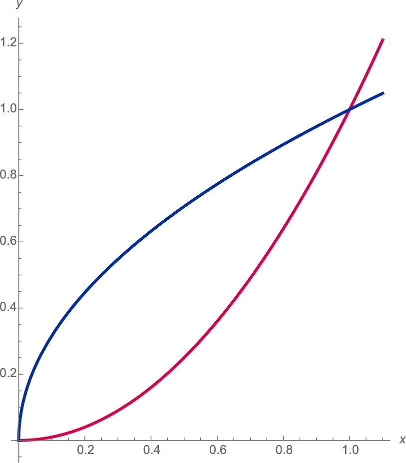
 , 0 ⩽ x ⩽ 1 (University of Arizona colors).
![]()
![]()
![]()
![]()
![]()
![]()
Using equation (5.14),
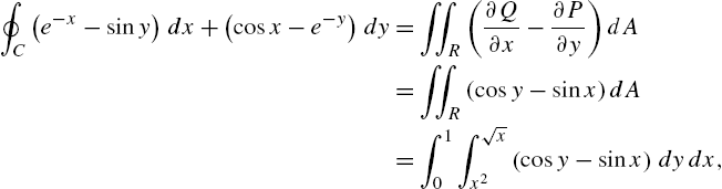
![]()
![]()
which we evaluate with Integrate.
![]()
![]()
![]()
0.151091
Notice that the result is given in terms of the FresnelS and FresnelC functions, which are defined by

A more meaningful approximation is obtained with N. We conclude that
□
5.5.3 Surface Integrals
Let S be the graph of ![]() (
(![]() ,
, ![]() ) and let
) and let ![]() (
(![]() ,
, ![]() ) be the projection of S onto the xy (xz, yz) plane. Then,
) be the projection of S onto the xy (xz, yz) plane. Then,


If S is defined parametrically by
the formula
where
is also useful.
Theorem 5.3
The Divergence Theorem
Let Q be any domain with the property that each line through any interior point of the domain cuts the boundary in exactly two points, and such that the boundary S is a piecewise smooth closed, oriented surface with unit normal n. If F is a vector field that has continuous partial derivatives on Q, then
In (5.19), ![]() is called the outward flux of the vector field F across the surface S. If S is a portion of the level curve
is called the outward flux of the vector field F across the surface S. If S is a portion of the level curve ![]() for some g, then a unit normal vector n may be taken to be either
for some g, then a unit normal vector n may be taken to be either
If S is defined parametrically by
a unit normal vector to the surface is ![]() and (5.19) becomes
and (5.19) becomes ![]() .
.
Example 5.42
Solution
By the Divergence theorem,

Hence, without the Divergence theorem, calculating the outward flux would require six separate integrals, corresponding to the six faces of the cube. After defining F, we compute ![]() with Div.
with Div.
![]()
![]()
![]()
Remember, “Cartesian” is the default coordinate system so the same result as that obtained above is obtained with the following commands. Also keep in mind that Mathematica understands a wide number of coordinate systems. Thus, if you need results in your coordinatesystem be sure to include the explicit system in your command.
![]()
![]()
The outward flux is then given by
which we compute with Integrate.
![]()
2 □
Theorem 5.4
Stokes' Theorem
In other words, the surface integral of the normal component of the curl of F taken over S equals the line integral of the tangential component of the field taken over C. In particular, if ![]() , then
, then

Example 5.43
Solution
The curl of F is computed with Curl in curlcapf.
![]()
![]()
![]()
![]()
Next, we define the function ![]() . A normal vector to the surface is given by ▽h. A unit normal vector, n, is then given by
. A normal vector to the surface is given by ▽h. A unit normal vector, n, is then given by ![]() , which is computed in un.
, which is computed in un.
![]()
![]()
![]()
![]()
![]()
![]()
The dot product ![]() is computed in g.
is computed in g.
![]()
![]()
Using the surface integral evaluation formula (5.15),

In this example, R, the projection of ![]() onto the xy-plane, is the region bounded by the graph of the circle
onto the xy-plane, is the region bounded by the graph of the circle ![]() .
.
which we compute with Integrate.
![]()
![]()
![]()
![]()
![]()
9π
To verify Stokes' theorem, we must compute the associated line integral. Notice that the boundary of ![]() ,
, ![]() , is the circle
, is the circle ![]() with parametrization
with parametrization ![]() ,
, ![]() ,
, ![]() ,
, ![]() . This parametrization is substituted into
. This parametrization is substituted into ![]() and named pvf.
and named pvf.
![]()
![]()
To evaluate the line integral along the circle, we next define the parametrization of the circle and calculate ![]() . The dot product of pvf and dr represents the integrand of the line integral.
. The dot product of pvf and dr represents the integrand of the line integral.
![]()
![]()
![]()
![]()
As before with x and y, we instruct Mathematica to assume that t is real, compute the dot product of pvf and dr, and evaluate the line integral with Integrate.
![]()
9π
As expected, the result is 9π. □
5.5.4 A Note on Nonorientability
Suppose that S is the surface determined by
and let
where
if ![]() . If n is defined, n is orthogonal (or perpendicular) to S. We state three familiar definitions of orientable.
. If n is defined, n is orthogonal (or perpendicular) to S. We state three familiar definitions of orientable.
• S is orientable if S has a unit normal vector field, n, that varies continuously between any two points ![]() and
and ![]() on S. (See [5].)
on S. (See [5].)
• S is orientable if S has a continuous unit normal vector field, n. (See [5] and [16].)
• S is orientable if a unit vector n can be defined at every nonboundary point of S in such a way that the normal vectors vary continuously over the surface S. (See [11].)
A path is order preserving if our chosen orientation is preserved as we move along the path.
Thus, a surface like a torus is orientable.
Example 5.44
The Torus
Using the standard parametrization of the torus, we use ParametricPlot3D to plot the torus if ![]() and
and ![]() in Fig. 5.14.
in Fig. 5.14.
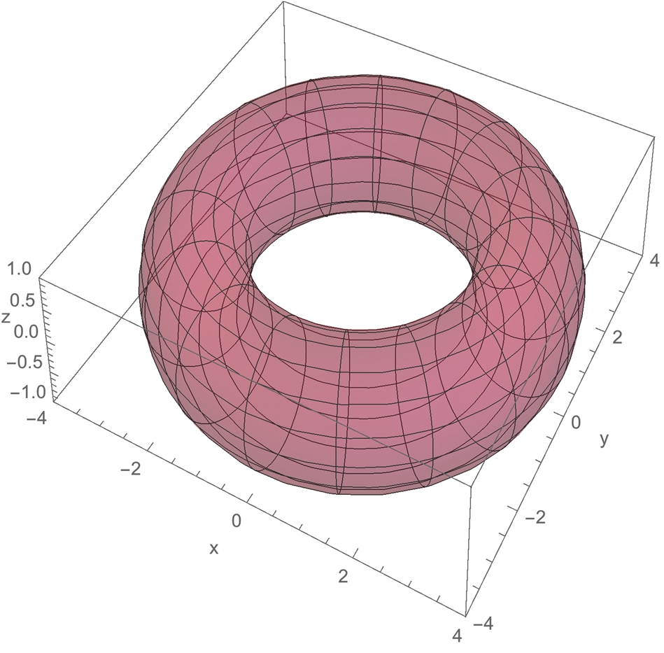
![]()
![]()
![]()
![]()
![]()
![]()
![]()
![]()
![]()
![]()
![]()
![]()
To plot a normal vector field on the torus, we compute ![]() ,
,
![]()
![]()
![]()
![]()
The cross product ![]() is formed in rscrossrt.
is formed in rscrossrt.
![]()
![]()
![]()
![]()
Using equation (5.24), we define un: given s and t, un[s,t] returns a unit normal to the torus.
![]()
![]()
![]()
![]()
![]()
![]()
![]()
![]()
![]()
![]()
![]()
To plot the normal vector field on the torus, we take advantage of the command Arrow. The command
Arrow[{{u1,u2,u3},{v1,v2,v3}}]
generates an arrow from ![]() to
to ![]() , which we interpret to be the vector going from
, which we interpret to be the vector going from ![]() to
to ![]() . To display the Arrow object, use Show together with Graphics (for two-dimensional arrows) or Graphics3D (for three dimensional arrows). See Fig. 5.15.
. To display the Arrow object, use Show together with Graphics (for two-dimensional arrows) or Graphics3D (for three dimensional arrows). See Fig. 5.15.

![]()
![]()
![]()
![]()
We use Show (illustrating the use of the ViewPoint option) together with GraphicsGrid to see the vector field on the torus together from various angles in Fig. 5.16. Regardless of the viewing angle, the figure looks the same; the torus is orientable.
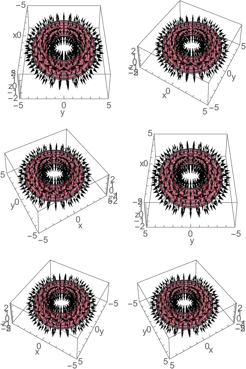
![]()
![]()
![]()
![]()
![]()
![]()
![]()
![]()
![]()
![]()
![]()
![]()
![]()
![]()
![]()
![]()
![]()
![]()
![]()
![]()
![]()
![]()
![]()
![]()
![]()
![]()
![]()
![]()
If a 2-manifold, S, has an order reversing path (or not order preserving path), S is nonorientable (or not orientable).
Determining whether a given surface S is orientable or not may be a difficult problem.
Example 5.45
The Möbius Strip
The Möbius strip is frequently cited as an example of a nonorientable surface with boundary: it has one side and is physically easy to construct by hand by half twisting and taping (or pasting) together the ends of a piece of paper (for example, see [5], [11], and [16]). A parametrization of the Möbius strip is ![]() ,
, ![]() ,
, ![]() , where
, where
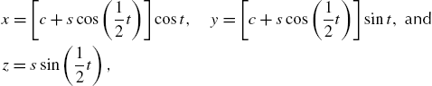
and we assume that ![]() . In Fig. 5.17, we graph the Möbius strip using
. In Fig. 5.17, we graph the Möbius strip using ![]() .
.
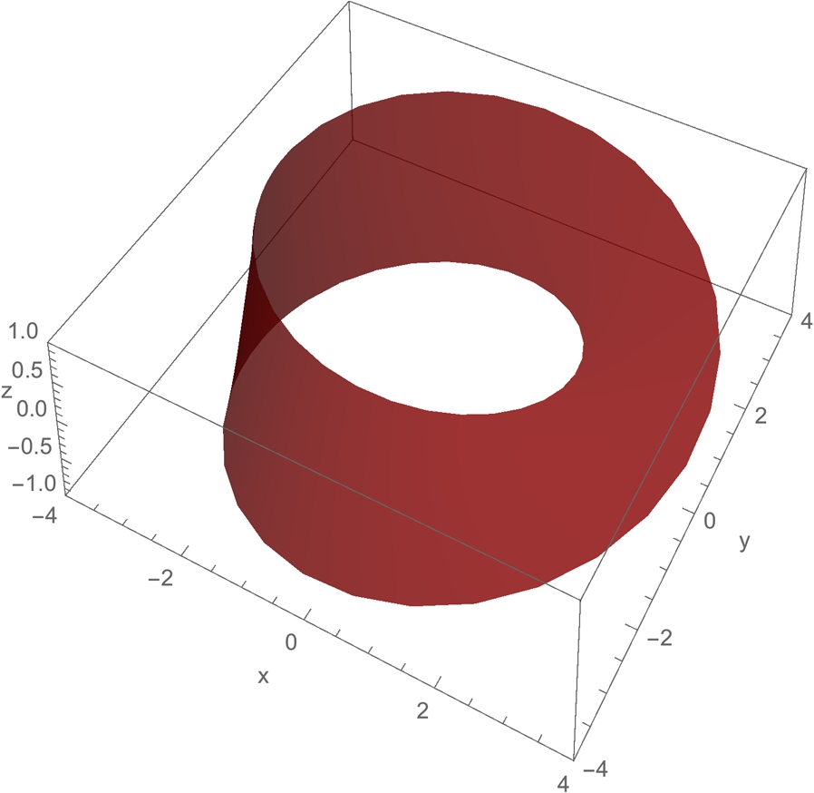
![]()
![]()
![]()
![]()
![]()
![]()
![]()
![]()
![]()
![]()
![]()
Although it is relatively easy to see in the plot that the Möbius strip has only one side, the fact that a unit vector, n, normal to the Möbius strip at a point P reverses its direction as n moves around the strip to P is not obvious to the novice.
With Mathematica, we compute ![]() and
and ![]() .
.
![]()
![]()
![]()
![]()
![]()
![]()
![]()
![]()
![]()
![]()
![]()
![]()
Consider the path C given by ![]() ,
, ![]() that begins and ends at
that begins and ends at ![]() . On C,
. On C, ![]() is given by
is given by
![]()
![]()
At ![]() ,
, ![]() , while at
, while at ![]() ,
, ![]() .
.
![]()
![]()
![]()
![]()
As n moves along C from ![]() to
to ![]() , the orientation of n reverses, as shown in Fig. 5.18.
, the orientation of n reverses, as shown in Fig. 5.18.
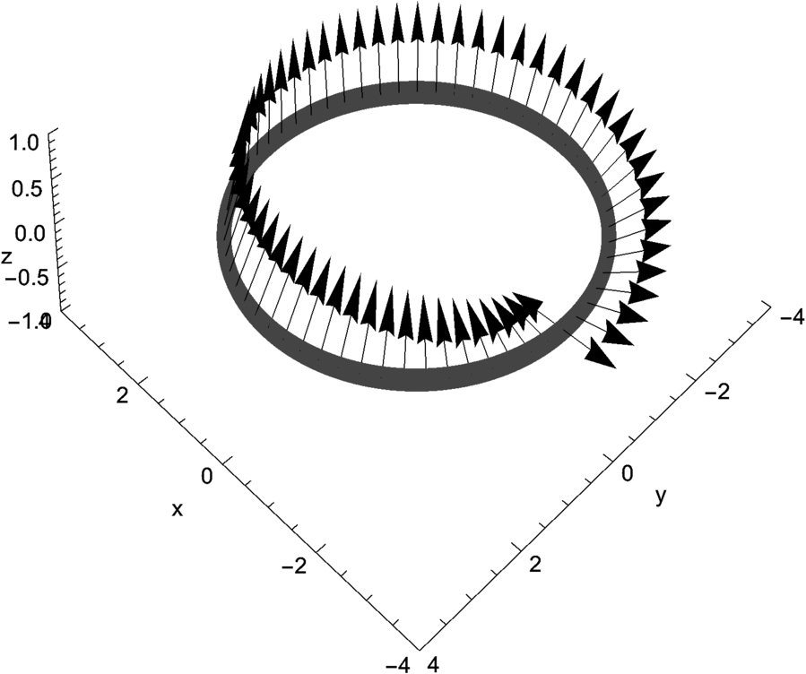
![]()
![]()
![]()
![]()
![]()
![]()
![]()
![]()
![]()
![]()
Several different views of Fig. 5.18 on the Möbius strip shown in Fig. 5.17 are shown in Fig. 5.19. C is an orientation reversing path and we can conclude that the Möbius strip is not orientable.
![]()
![]()
![]()
![]()
![]()
![]()
![]()
![]()
![]()
![]()
![]()
![]()
![]()
![]()
![]()
![]()
![]()
![]()
![]()
Example 5.46
The Klein bottle is an interesting surface with neither an inside nor an outside, which indicates to us that it is not orientable. In Fig. 5.20 (a) we show the “usual” immersion of the Klein bottle. Although the Klein bottle does not intersect itself, it is not possible to visualize it in Euclidean 3-space without it doing so. Visualizations of 2-manifolds like the Klein bottle's “usual” rendering in Euclidean 3-space are called immersions. (See [14] for a nontechnical discussion of immersions.)
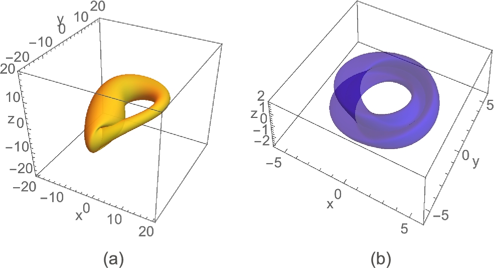
![]()
![]()
![]()
![]()
![]()
![]()
![]()
![]()
![]()
![]()
![]()
![]()
![]()
![]()
![]()
Fig. 5.20 (b) shows the Figure-8 immersion of the Klein bottle. Notice that it is not easy to see that the Klein bottle has neither an inside nor an outside in Fig. 5.14.
![]()
![]()
![]()
![]()
![]()
![]()
![]()
![]()
![]()
![]()
![]()
![]()
In fact, to many readers it may not be clear whether the Klein bottle is orientable or nonorientable, especially when we compare the graph to the graphs of the Möbius strip and torus in the previous examples.
A parametrization of the Figure-8 immersion of the Klein bottle (see [17]) is ![]() ,
, ![]() ,
, ![]() , where
, where

The plot in Fig. 5.20 (b) uses equation (5.23) if ![]() .
.
Using (5.21), let
Let C be the path given by
that begins and ends at ![]() and where the components are given by (5.23). The components of r and n are computed with Mathematica. The final calculations are quite lengthy so we suppress the output of the last few by placing a semicolon (;) at the end of those commands.
and where the components are given by (5.23). The components of r and n are computed with Mathematica. The final calculations are quite lengthy so we suppress the output of the last few by placing a semicolon (;) at the end of those commands.
![]()
![]()
![]()
![]()
![]()
![]()
![]()
![]()
At ![]() ,
, ![]() , while at
, while at ![]() ,
, ![]() so as n moves along C from
so as n moves along C from ![]() to
to ![]() , the orientation of n reverses. Several different views of the orientation reversing path on the Klein bottle shown in Fig. 5.20 (b) are shown in Fig. 5.21.
, the orientation of n reverses. Several different views of the orientation reversing path on the Klein bottle shown in Fig. 5.20 (b) are shown in Fig. 5.21.
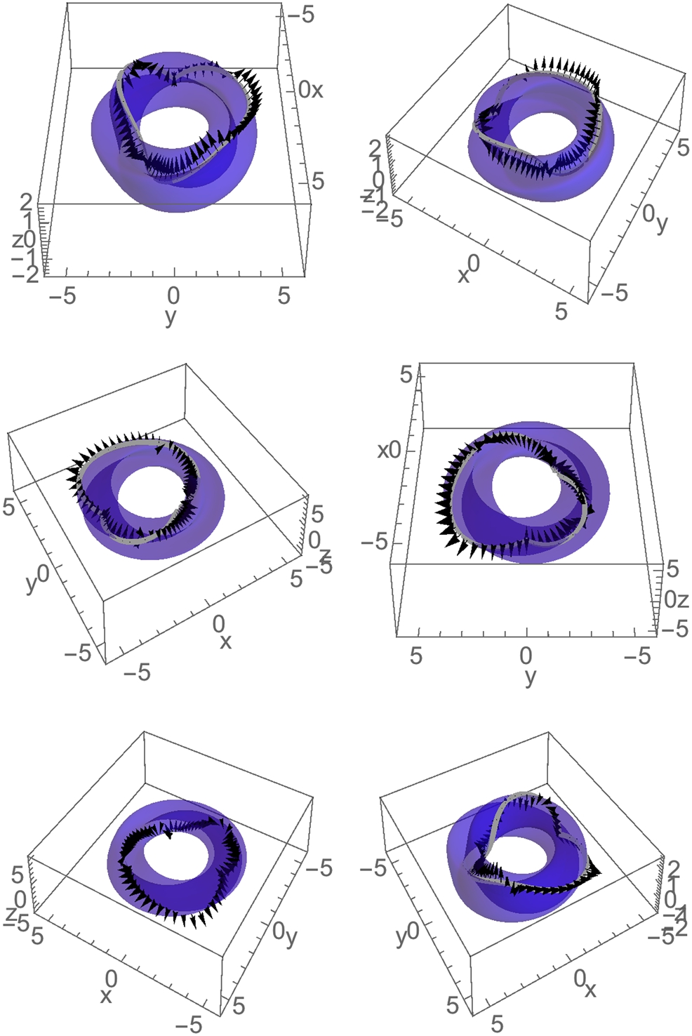
![]()
![]()
![]()
![]()
![]()
![]()
![]()
![]()
![]()
![]()
![]()
![]()
![]()
![]()
![]()
![]()
![]()
![]()
![]()
![]()
![]()
![]()
![]()
![]()
![]()
![]()
![]()
![]()
![]()
![]()
![]()
![]()
![]()
![]()
![]()
![]()
![]()
![]()
C is an orientation reversing path and we can conclude that the Klein bottle is not orientable.
5.5.5 More on Tangents, Normals, and Curvature in R 3 
Earlier, we discussed the unit tangent and normal vectors and curvature for a vector-valued function ![]() . These concepts can be extended to curves and surfaces in space.
. These concepts can be extended to curves and surfaces in space.
For ![]() , the Frenet frame field is the ordered triple
, the Frenet frame field is the ordered triple ![]() , where T is the unit tangent vector field, N is the unit normal vector field, and B is the unit binormal vector field. Each of these vectors has norm 1 and each is orthogonal to the other (the dot product of one with another is 0) and the Frenet formulas are satisfied:
, where T is the unit tangent vector field, N is the unit normal vector field, and B is the unit binormal vector field. Each of these vectors has norm 1 and each is orthogonal to the other (the dot product of one with another is 0) and the Frenet formulas are satisfied: ![]() ,
, ![]() ,
, ![]() . τ is the torsion of the curve γ; κ is the curvature. For the curve
. τ is the torsion of the curve γ; κ is the curvature. For the curve ![]() , formulas for these quantities are given by:
, formulas for these quantities are given by:

We adjust Gray's routines slightly for Mathematica 11. Here is the unit tangent vector,
![]()
![]()
Similarly, the binormal is defined with
![]()
![]()
![]()
![]()
so the unit normal is defined with
![]()
Notice how we use Assumptions to instruct Mathematica to assume that the domain of γ consists of real numbers. In the same manner, we define the curvature and torsion.
![]()
![]()
![]()
![]()
![]()
![]()
![]()
![]()
In even the simplest situations, these calculations are quite complicated. Graphically seeing the results may be more meaningful that the explicit formulas.
Example 5.47
Consider the spherical spiral given by ![]() . The curvature and torsion for the curve are graphed with Plot and shown in Fig. 5.22.
. The curvature and torsion for the curve are graphed with Plot and shown in Fig. 5.22.
![]()
![]()
![]()
![]()
![]()
We now compute T, B, and N. For length considerations, we display an abbreviated portion of B with Short.
![]()
![]()
![]()
![]()
![]()
![]()
It is difficult to see how these complicated formulas relate to this spherical spiral. To help us understand what they mean, we first plot the spiral with ParametricPlot3D. See Fig. 5.23 (a).
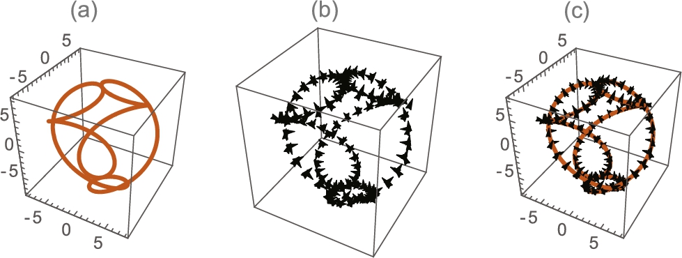
![]()
![]()
![]()
Next, we use Table to compute lists of two ordered triples. For each list, the first ordered triple consists of ![]() and the second the value of the sum of
and the second the value of the sum of ![]() and
and ![]() (
(![]() ,
, ![]() ). These ordered triples that correspond to vectors are plotted with Arrow together with Show and Graphics3D.
). These ordered triples that correspond to vectors are plotted with Arrow together with Show and Graphics3D.
![]()
![]()
![]()
![]()
![]()
![]()
![]()
For a nice view of p1 and p2, display them together with Show. See Fig. 5.23 (c).
![]()
![]()
The previous example illustrates that capturing the depth of three-dimensional curves by projections into two dimensions can be difficult. Sometimes taking advantage of three-dimensional surface plots can help. For a basic space curve, tubecurve places a “tube” of radius r around the space curve.
![]()
![]()
![]()
To illustrate the utility, we redefine torusknot that was presented in Chapter 2.
![]()
![]()
![]()
Example 5.48
For the knot torusknot}[8,3,5][2,5] we plot the curvature and torsion with Plot in Fig. 5.24.
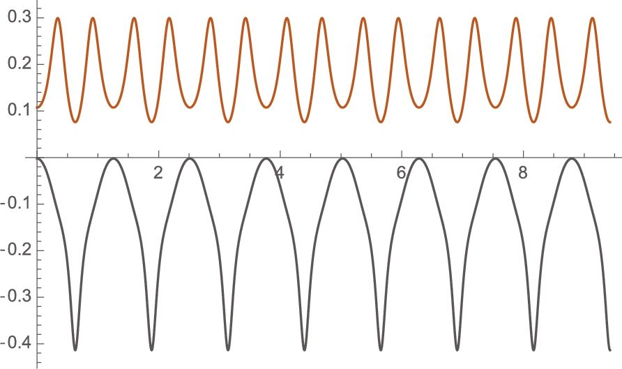
![]()
![]()
![]()
![]()
We generate a basic plot of this torus knot in 3-space with ParametricPlot3D. See Fig. 5.25 (a).
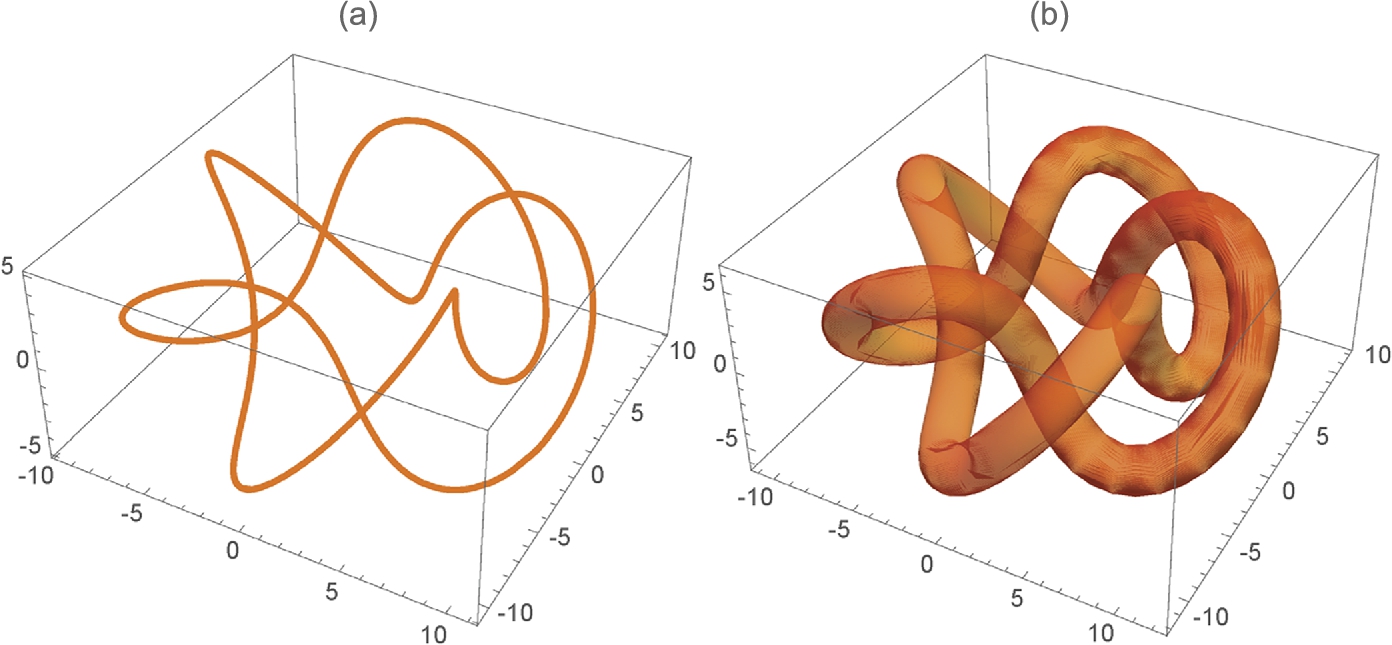
![]()
![]()
Using tubecurve, we place a “tube” around the knot. See Fig. 5.25 (b).
![]()
![]()
![]()
![]()
A more interesting graphic is obtained by placing a transparent tube around the curve
![]()
![]()
![]()
![]()
and then creating a thicker version of the curve.
![]()
![]()
As before, we use tangent, normal, and binormal to create a vector field on the curve.
![]()
![]()
![]()
![]()
![]()
![]()
![]()
![]()
![]()
A striking graph is generated by showing the three graphs together. See Fig. 5.26
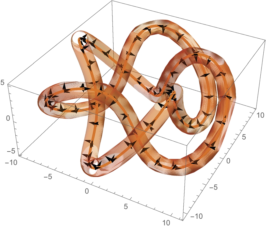
![]()
![]()
![]()
![]()
![]()
Alternatively, display the results as an array with GraphicsGrid. See Fig. 5.27.
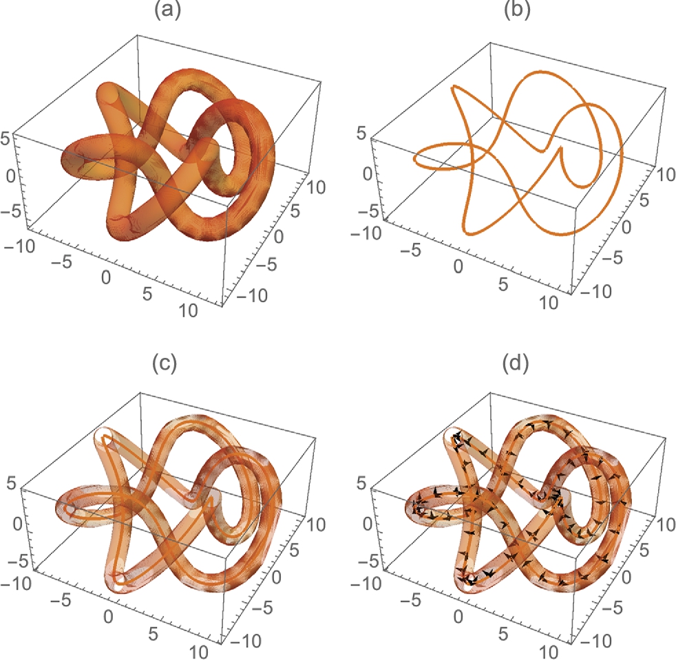
![]()
Example 5.49
The Trefoil knot is the special case of torusknot[8,3,5][2,3]][t]. We use Plot to graph its curvature and torsion in Fig. 5.28. Because we have used Tooltip, you can identify each plot by moving the cursor over the curve in Fig. 5.28.
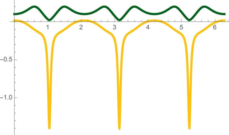
![]()
![]()
![]()
![]()
Next, we generate a thickened version of the Trefoil knot.
![]()
![]()
Three different tube plots of the Trefoil knot are generated. In p2, the result is a basic plot. In p2b, The plot is shaded according to the Rainbow color gradient. In p2c, the plot is shaded according to the knots curvature. The knot together with the three surfaces are shown together in Fig. 5.29.
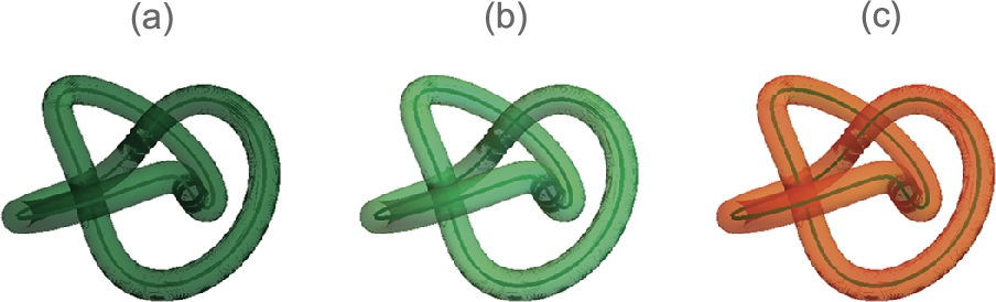
![]()
![]()
![]()
![]()
![]()
![]()
![]()
![]()
![]()
![]()
![]()
![]()
![]()
For surfaces in ![]() , extending and stating these definitions precisely becomes even more complicated. First, define the vector triple product (xyz), where
, extending and stating these definitions precisely becomes even more complicated. First, define the vector triple product (xyz), where  ,
,  , and
, and  , by
, by  . We assume that
 ![]() is a vector-valued function with domain contained in a “nice” region
is a vector-valued function with domain contained in a “nice” region ![]() and range in
and range in ![]() . The Gaussian curvature,
. The Gaussian curvature, ![]() , and the mean curvature,
, and the mean curvature, ![]() , under reasonable conditions, are given by the formulas
, under reasonable conditions, are given by the formulas
For the parametrically defined surface ![]() , the unit normal field, U, is
, the unit normal field, U, is ![]() . Observe that the expressions that result from explicitly computing U,
. Observe that the expressions that result from explicitly computing U, ![]() , and
, and ![]() are almost always so complicated that they are impossible to understand.
are almost always so complicated that they are impossible to understand.
After defining vtp to return the vector triple product of three vectors, we define gaussianc and meanc to compute ![]() and
and ![]() for a parametrically defined surface
for a parametrically defined surface ![]() .
.
![]()
![]()
![]()
![]()
![]()
![]()
![]()
![]()
![]()
![]()
![]()
![]()
]
![]()
![]()
![]()
![]()
![]()
![]()
![]()
![]()
![]()
![]()
![]()
![]()
![]()
]
Example 5.50
We illustrate the commands with the torus, first discussed in Chapter 2, and ParametricPlot3D. For convenience, we redefine torus.
![]()
![]()
In pp1, we generate a basic plot of the torus. The shading is changed in pp2. In pp3 the surface is shaded according to its Gaussian curvature while in pp4 the surface is shaded according to its mean curvature. All four plots are shown together in Fig. 5.30.
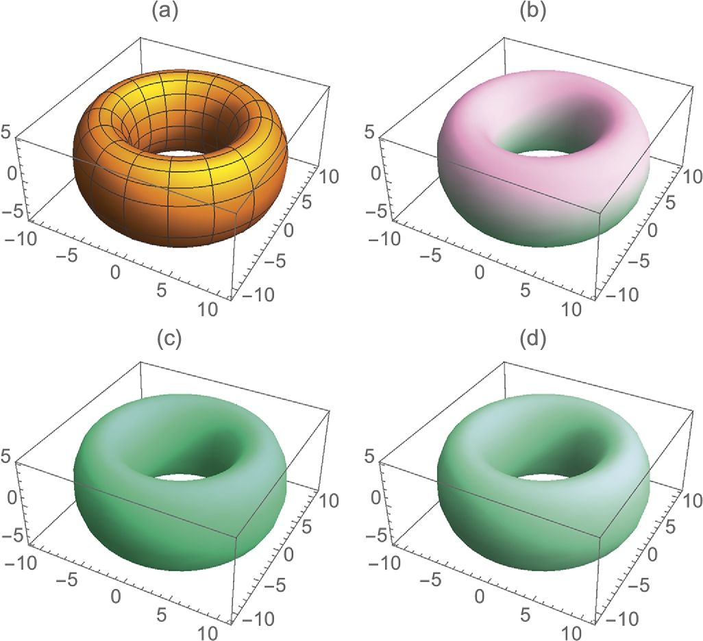
![]()
![]()
![]()
![]()
![]()
![]()
![]()
![]()
![]()
![]()
![]()
![]()
![]()
![]()
![]()
![]()
![]()
![]()
5.6 Matrices and Graphics
5.6.1 Manipulating Photographs with Built-In Functions
As introduced in Chapter 2, Mathematica contains a wide range of functions that allow you to manipulate images such as photographs quickly to achieve a variety of photographic effects.
To import a photograph or other image into Mathematica, use Import. Generally, the object that is to be imported should be in your root directory. However, Mathematica supports clicking and dragging: you can simply click on the file and drag it to the desired location in your Mathematica notebook.
For “standard” effects and manipulation of photographs, try using ImageEffect first. ImageEffect is fast and has a wide range of options. We illustrate just a few here. First, we import a graphic,
![]()
![]()

Next, we use ImageEffect to apply a variety of commonly used enhancements to the image, p1. The results are shown in Fig. 5.31.

![]()
![]()
![]()
![]()
![]()
Once you have imported an image either using Import or by selecting and dragging the image into the desired location in your Mathematica notebook, Mathematica gives you a wide range of functions to obtain information about the image.
![]()
![]()

To determine the size of your image, number of pixel columns by number of pixel rows, use ImageDimensions.
![]()
![]()
Here, we illustrate ImageAdjust with a few of its options (see Fig. 5.32).

![]()
![]()
![]()
![]()
ColorQuantize[image,n] approximates image with n colors. To see the resulting colors, use DominantColors. Observe that the colors are displayed in small squares.
![]()

To see the RGB code, click on the color or use InputForm to see the actual color codes displayed as a list.
![]()
![]()
ImageApply may give the most flexibility for dealing with a graphic as it allows you to manipulate the graphic pixel-by-pixel. Closely related commands to those discussed include ImageFilter, ImageConvolve, and ImageCorrelate. Use ?<command> to obtain detailed help regarding the capabilities of each (see Fig. 5.33).

![]()
![]()
![]()
![]()
![]()
![]()
5.6.2 Manipulating Photographs by Viewing Them as a Matrix or Array
With Mathematica, virtually every object is a list or list of lists, including images. In situations where you want to manipulate your image or photograph with more detail than that provided by the built-in Mathematica functions for manipulating Image objects, you may want to manipulate the data that determines the image directly. To do so, it is important to understand that the underlying data of an Image object is generally a matrix. Typically, the entries of the matrix for the image are single digits for black-and-white images or ordered triples of the form {r,g,b} for color jpegs. The easiest way to determine the size of the image is to use ImageDimensions[image]. The resulting list {n,m} indicates that the dimensions of image are n pixels of rows by m pixels of columns.
Mathematica contains several functions that allow you to represent matrices graphically. These commands are analogous to the corresponding ones for dealing with lists (like ListPlot) or functions (such as Plot, Plot3D, and ContourPlot).
1. MatrixPlot[A] generates a grid with the same dimensions as A. The cells are shaded according to the entries of A. The default is in color.
2. ArrayPlot[A] generates a grid with the same dimensions as A. The cells are shaded according to the entries of A. The default is in black and white.
3. ListContourPlot[A] generates a contour plot using the entries of A as the height values.
4. ReliefPlot[A] generates a relief plot using the entries of A as the height values.
Observe that ArrayPlot and MatrixPlot are virtually interchangeable. However, the entries of ArrayPlot need not be numbers. If Mathematica cannot determine how to shade a cell, the default is to shade it in a dark maroon color. Although these functions generate graphics that depend on the entries of the matrix, loosely speaking we will use phrases like “we use MatrixPlot to plot A” and “we use ArrayPlot to graph A” to describe the graphic that results from applying one of these functions to an array.
For example, consider the arrays  ,
, 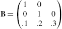 , and
, and ![]() .
.
In the first command, Mathematica shades all the cells according to its GrayLevel value. However, in the second and third commands, Mathematica cannot shade the cells in the second row and all the cells, respectively, because ordered triples cannot be evaluated by GrayLevel. However, RGBColor evaluates ordered triples so Mathematica shades the cells in Fig. 5.34 (c) according to their RGBColor value. See Fig. 5.34.

![]()
![]()
![]()
![]()
![]()
![]()
![]()
![]()
MatrixPlot is unable to graphically represent B or C. However, coloring is automatic with MatrixPlot. See Fig. 5.35.
![]()
![]()
![]()
![]()
If you need to adjust the color of a graphic, usually you can use the ColorSchemes palette to select an appropriate gradient or color function. In other situations, you might wish to create your own using Blend. To use Blend, you might need to know how various RGBColors or CMYKColors vary as the variables affecting the color change.
ArrayPlot can help us see the variability in the colors. With the following, we see how RGBColor[r,g,b] affects color for ![]() ,
, ![]() , and then
, and then ![]() . The results are shown together in Fig. 5.36. The figure can help us select appropriate values to generate our own color blending function using Blend rather than relying on Mathematica's built-in color schemes and gradients.
. The results are shown together in Fig. 5.36. The figure can help us select appropriate values to generate our own color blending function using Blend rather than relying on Mathematica's built-in color schemes and gradients.

In these calculations, t1 is a ![]() array for which each entry is an ordered triple. In the first t1, the ordered triple has the form
array for which each entry is an ordered triple. In the first t1, the ordered triple has the form ![]() , in the second the form
, in the second the form ![]() , and so on.
, and so on.
![]()
![]()
![]()
![]()
![]()
![]()
![]()
![]()
![]()
![]()
![]()
![]()
![]()
We modify the calculation slightly to see how CMYKColor varies as we adjust two parameters. Keep in mind that each t2 is a ![]() array. Each entry of t2 is an ordered quadruple, which is illustrated in the first calculation where we use Part to take the 5th element of the 8th part of t2 (see Fig. 5.37).
array. Each entry of t2 is an ordered quadruple, which is illustrated in the first calculation where we use Part to take the 5th element of the 8th part of t2 (see Fig. 5.37).
![]()
![]()
![]()
![]()
![]()
![]()
![]()
![]()
![]()
![]()
![]()
![]()
![]()
![]()
![]()
![]()
![]()
![]()
![]()
![]()
![]()
Keep in mind that you can load files into Mathematica with Import or by clicking and dragging the image to the desired location in your Mathematica notebook. Generally, the underlying structure of the loaded file is relatively easy to understand. Be careful when you import data into Mathematica. We recommend that you use ExampleData to investigate your routines before finalizing them. Although importing external files into Mathematica is easy, understanding the underlying structure of the imported data may take some time but be necessary to produce the results you desire.
We illustrate a few of the subtle differences that can be encountered with several images.
Using Import, we import a graphic into Mathematica. The result is shown in Fig. 5.38 (a).
![]()
![]()

We use ImageDimensions to determine the size of the image.
![]()
![]()
Alternatively, using Length we see that p2 has 439 rows (pixels)
![]()
439
and then counting the number of entries in the first row of p2, we see that p2 has 640 columns (pixels).
![]()
640
To convert the image to an array (matrix) that we can manipulate, we use ImageData.
![]()
After we have obtained the image data from p1 in p2, we see that it is a matrix where each entry is a list of the form ![]() , corresponding to the RGB color code for that pixel.
, corresponding to the RGB color code for that pixel.
![]()
![]()
ArrayPlot produces the negative of an image. See Fig. 5.38 (a).
![]()
To manipulate p2, it is important to understand that p2 is a ![]() array where each entry is a
array where each entry is a ![]() list, corresponding to the RGB color codes for that particular pixel.
list, corresponding to the RGB color codes for that particular pixel.
![]()
![]()
![]()
640
To convert the image to a different color, we first convert the matrix to a list of ordered triples, p3, define ![]() , apply f to p3, and then apply a color function to the result. In this example, we chose to use the Rainbow color function.
, apply f to p3, and then apply a color function to the result. In this example, we chose to use the Rainbow color function.
![]()
![]()
![]()
![]()
![]()
![]()
![]()
We show the results in Fig. 5.38. On a color printer, the results are amazing.
![]()
![]()
The results are shown side-by-side in Fig. 5.38. Printed on a color printer, the results are amazing.
![]()
Now that we understand how to manipulate an image, we can be creative. In the following, the image is scaled so that the width of the image is 70 pixels (because of ImageSize->70). We then display the small image with another graphic. Using Inset, we put the Colliseum next to a sine graph that is plotted using the same coloring gradient. See Fig. 5.39.
![]()
![]()
![]()
An alternative way to visualize the data is to use ListContourPlot. To assure that the aspect ratio of the original image is preserved, include the AspectRatio->Automatic option in the ListContourPlot command (see Fig. 5.40).

![]()
![]()
![]()
![]()
![]()
![]()
The structure of a black and white jpeg differs from that of a color one. To see so, we import a very old picture of the second author of this text,
![]()
![]()
and name the result p1. With ImageDimensions, we see that p1 is 428 pixels wide by 600 pixels tall.
![]()
![]()
We obtain the data for the image with ImageData. With Length, we see that the resulting array has 600 rows and 428 columns, confirming the result obtained with ImageDimensions. Using Short, we see the form of each entry. For the black-and-white image, each entry is a number that corresponds to a GrayLevel.
![]()
![]()
600
![]()
428
![]()
![]()
In Fig. 5.41, we illustrate the use of ListContourPlot and ReliefPlot along with various options.
![]()
![]()
![]()
![]()
![]()
![]()
![]()
![]()
ReliefPlot can help add insight to images, especially when they have geographical or biological meaning. For example, this jpeg
![]()
![]()
shows the beginning of a biological process of a cell.
With ImageDimensions, we see that p1 is a 400 pixels wide by 500 pixels tall. After obtaining the image data with ImageData, these calculations are confirmed with length.
![]()
![]()
![]()
![]()
500
![]()
500
![]()
400
Viewing p2 as a ![]() array, each entry is
array, each entry is ![]() array/vector. To easily apply a function, f, that assigns a number to each ordered triple, we use Flatten to convert the nested list/array p2 to a list of ordered triples in p3.
array/vector. To easily apply a function, f, that assigns a number to each ordered triple, we use Flatten to convert the nested list/array p2 to a list of ordered triples in p3.
![]()
![]()
![]()
200000
![]()
To apply our own color function to this data set, we convert the ordered triples to some other form. For illustrative purposes, we convert each ordered triple ![]() in p3 to the number
in p3 to the number ![]() . The result is converted back to a
. The result is converted back to a ![]() array, with Partition in p4.
array, with Partition in p4.
![]()
![]()
![]()
500
We then use ReliefPlot, ListContourPlot, and ListDensityPlot along with various options to graph the result in Fig. 5.42.
![]()
![]()
![]()
![]()
![]()
![]()
![]()
![]()
![]()
![]()
![]()