Basic Operations on Numbers, Expressions, and Functions
Keywords
Operations on numbers; Operations on functions; Two-dimensional graphics; Three-dimensional graphics; Image processing
2.1 Numerical Calculations and Built-In Functions
2.1.1 Numerical Calculations
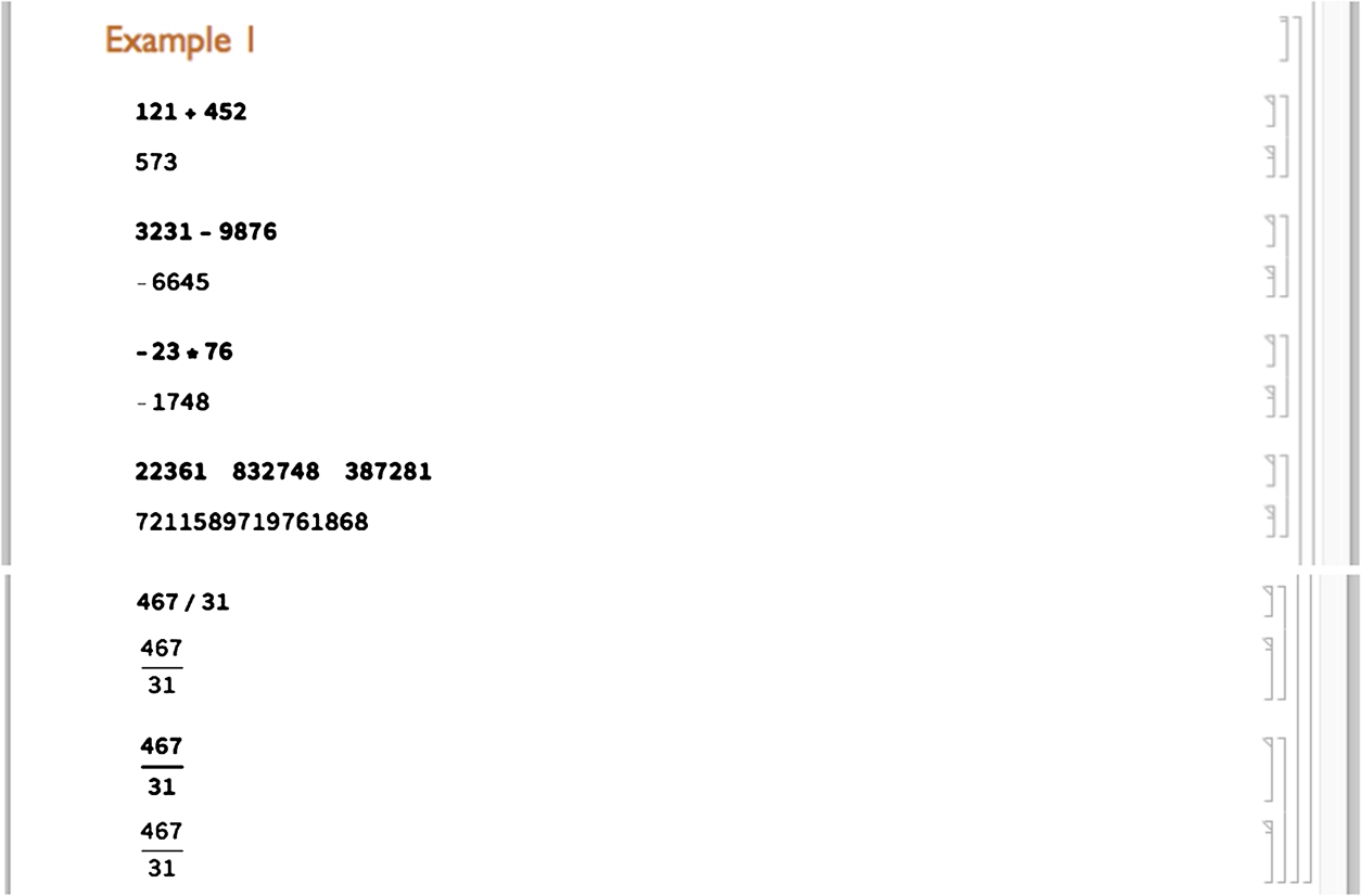
The basic arithmetic operations (addition, subtraction, multiplication, division, and exponentiation) are performed in the natural way with Mathematica. Whenever possible, Mathematica gives an exact answer and reduces fractions.
1. “a plus b,” ![]() , is entered as a+b;
, is entered as a+b;
2. “a minus b,” ![]() , is entered as a-b;
, is entered as a-b;
3. “a times b,” ab, is entered as either a*b or a b (note the space between the symbols a and b);
4. “a divided by b,” ![]() , is entered as a/b. Executing the command a/b results in a fraction reduced to lowest terms; and
, is entered as a/b. Executing the command a/b results in a fraction reduced to lowest terms; and
5. “a raised to the bth power,” ![]() , is entered as a^b.
, is entered as a^b.
Example 2.1
Calculate (a) ![]() ; (b)
; (b) ![]() ; (c)
; (c) ![]() ; (d)
; (d) ![]() ; and (e)
; and (e) ![]() .
.
Solution
These calculations are carried out in the following screen shot. In each case, the input is typed and then evaluated by pressing Enter. In the last case, the Basic Math template is used to enter the fraction.
□
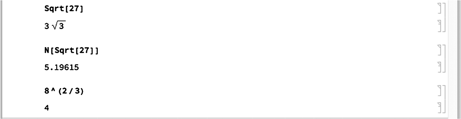
The term ![]() is entered as a^(n/m). For
is entered as a^(n/m). For ![]() , the command Sqrt[a] can be used instead. Usually, the result is returned in unevaluated form but N can be used to obtain numerical approximations to virtually any degree of accuracy. With N[expr,n], Mathematica yields a numerical approximation of expr to n digits of precision, if possible. At other times, Simplify can be used to produce the expected results.
, the command Sqrt[a] can be used instead. Usually, the result is returned in unevaluated form but N can be used to obtain numerical approximations to virtually any degree of accuracy. With N[expr,n], Mathematica yields a numerical approximation of expr to n digits of precision, if possible. At other times, Simplify can be used to produce the expected results.
Remark 2.1
If the expression b in ![]() contains more than one symbol, be sure that the exponent is included in parentheses. Entering a^n/m computes
contains more than one symbol, be sure that the exponent is included in parentheses. Entering a^n/m computes ![]() while entering a^(n/m) computes
while entering a^(n/m) computes ![]() .
.
Example 2.2
Compute (a) ![]() and (b)
and (b) ![]() .
.
Solution
(a) Mathematica automatically simplifies ![]() . We use N to obtain an approximation of
. We use N to obtain an approximation of ![]() . (b) Mathematica automatically simplifies
. (b) Mathematica automatically simplifies ![]() .
.
 □
□
When computing odd roots of negative numbers, Mathematica's results are surprising to the novice. Namely, Mathematica returns a complex number. We will see that this has important consequences when graphing certain functions.
Example 2.3
Calculate (a) ![]() and (b)
and (b) ![]() .
.
Solution
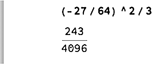
(a) Because Mathematica follows the order of operations, (-27/64)^2/3 first computes ![]() and then divides the result by 3.
and then divides the result by 3.
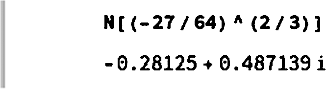
(b) On the other hand, (-27/64)^(2/3) raises ![]() to the 2/3 power. Mathematica does not automatically simplify
to the 2/3 power. Mathematica does not automatically simplify ![]() .
.

However, when we use N, Mathematica returns the numerical version of the principal root of ![]() .
.
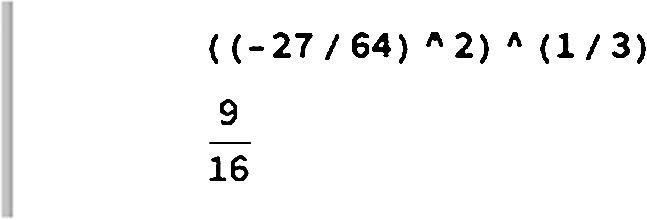
To obtain the result
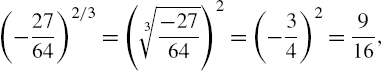
which would be expected by most algebra and calculus students, we first square ![]() and then take the third root.
and then take the third root.
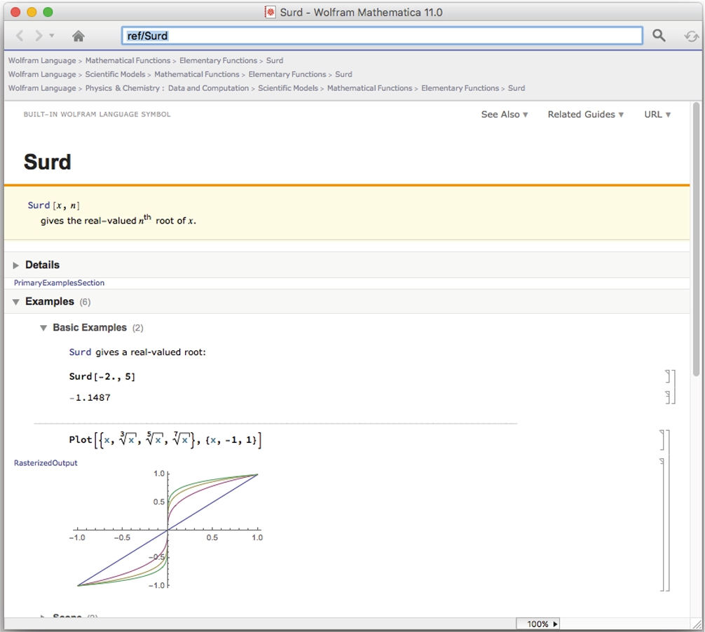
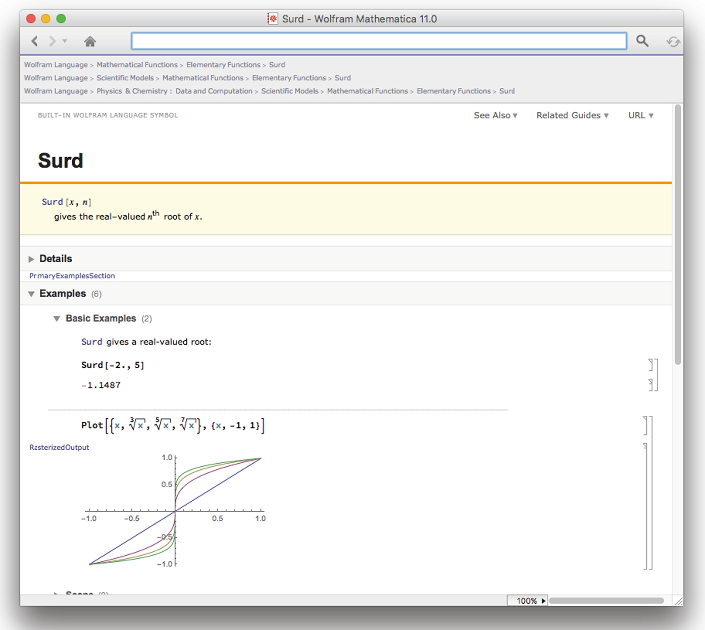
The Surd function automatically returns the real-valued nth root of x that most beginning users of Mathematica expect.
Then,
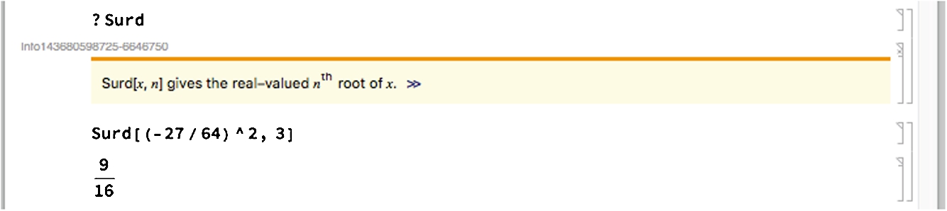
returns the result 9/16. □
2.1.2 Built-In Constants
Mathematica has built-in definitions of nearly all commonly used mathematical constants and functions. To list a few, ![]() is denoted by E,
is denoted by E, ![]() is denoted by Pi, and
is denoted by Pi, and ![]() is denoted by I. Usually, Mathematica performs complex arithmetic automatically.
is denoted by I. Usually, Mathematica performs complex arithmetic automatically.
Other built-in constants include ∞, denoted by Infinity, Euler's constant, ![]() , denoted by EulerGamma, Catalan's constant, approximately 0.915966, denoted by Catalan, and the golden ratio,
, denoted by EulerGamma, Catalan's constant, approximately 0.915966, denoted by Catalan, and the golden ratio, ![]() , denoted by GoldenRatio.
, denoted by GoldenRatio.
Example 2.4
Entering
![]()
2.7182818284590452353602874713526624977572470937000
returns a 50-digit approximation of e. Entering
![]()
3.141592653589793238462643
returns a 25-digit approximation of π. Entering
![]()
![]()
performs the division ![]() and writes the result in standard form.
and writes the result in standard form.
2.1.3 Built-In Functions
Functions frequently encountered by beginning users include the exponential function, Exp[x]; the natural logarithm, Log[x]; the absolute value function, Abs[x]; the trigonometric functions Sin[x], Cos[x], Tan[x], Sec[x], Csc[x], and Cot[x]; the inverse trigonometric functions ArcSin[x], ArcCos[x], ArcTan[x], ArcSec[x], ArcCsc[x], and ArcCot[x]; the hyperbolic trigonometric functions Sinh[x], Cosh[x], and Tanh[x]; and their inverses ArcSinh[x], ArcCosh[x], and ArcTanh[x]. Generally, Mathematica tries to return an exact value unless otherwise specified with N.
Several examples of the natural logarithm and the exponential functions are given next. Mathematica often recognizes the properties associated with these functions and simplifies expressions accordingly.
Example 2.5
Entering
![]()
![]()
![]()
0.00673795
returns an approximation of ![]() . Entering
. Entering
Exp[x] computes ![]() . Enter E to compute
. Enter E to compute ![]() .
.
![]()
3
computes ![]() . Entering
. Entering
Log[x] computes ![]() .
. ![]() and
and ![]() are inverse functions (
are inverse functions (![]() and
and ![]() ) and Mathematica uses these properties when simplifying expressions involving these functions.
) and Mathematica uses these properties when simplifying expressions involving these functions.
![]()
π
computes ![]() . Entering
. Entering
![]()
5
computes ![]() . Entering
. Entering
Abs[x] returns the absolute value of x, ![]() .
.
![]()
![]()
computes ![]() . Entering
. Entering
![]()
![]()
![]()
0.965926
computes the exact value of ![]() and then an approximation. Although Mathematica cannot compute the exact value of
and then an approximation. Although Mathematica cannot compute the exact value of ![]() , entering
, entering
![]()
1.47032
returns an approximation of ![]() . Similarly, entering
. Similarly, entering
![]()
0.339837
returns an approximation of ![]() and entering
and entering
![]()
0.841069
returns an approximation of ![]() .
.
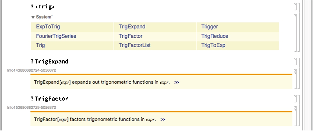
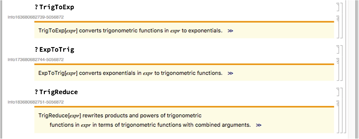
Mathematica is able to apply many identities that relate the trigonometric and exponential functions using the functions TrigExpand, TrigFactor, TrigReduce, TrigToExp, and ExpToTrig.
Example 2.6
Mathematica does not automatically apply the identity ![]() .
.
![]()
![]()
To apply the identity, we use Simplify. Generally, Simplify[expression] attempts to simplify expression.
![]()
1
Use TrigExpand to multiply expressions or to rewrite trigonometric functions. In this case, entering
Many of the algebraic manipulation commands can be accessed from the AlgebraicManipulation palette.

![]()
![]()
writes ![]() in terms of trigonometric functions with argument x. We use the TrigReduce function to convert products to sums.
in terms of trigonometric functions with argument x. We use the TrigReduce function to convert products to sums.
![]()
![]()
We use TrigExpand to write
![]()
![]()
![]()
![]()
in terms of trigonometric functions with argument x. We use ExpToTrig to convert exponential expressions to trigonometric expressions.
![]()
![]()
Similarly, we use TrigToExp to convert trigonometric expressions to exponential expressions.
![]()
![]()
Usually, you can use Simplify to apply elementary identities.
![]()
![]()
A Word of Caution
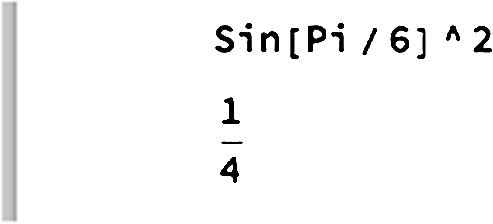
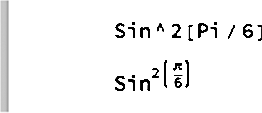
Remember that there are certain ambiguities in traditional mathematical notation. For example, the expression ![]() is usually interpreted to mean “compute
is usually interpreted to mean “compute ![]() and square the result.” That is,
and square the result.” That is, ![]() . The symbol sin is not being squared; the number
. The symbol sin is not being squared; the number ![]() is squared. With Mathematica, we must be especially careful and follow the standard order of operations exactly, especially when using InputForm. We see that entering
is squared. With Mathematica, we must be especially careful and follow the standard order of operations exactly, especially when using InputForm. We see that entering
computes ![]() while
while
raises the symbol Sin to the power ![]() . Mathematica interprets
. Mathematica interprets ![]() to be the product of the symbols sin2 and
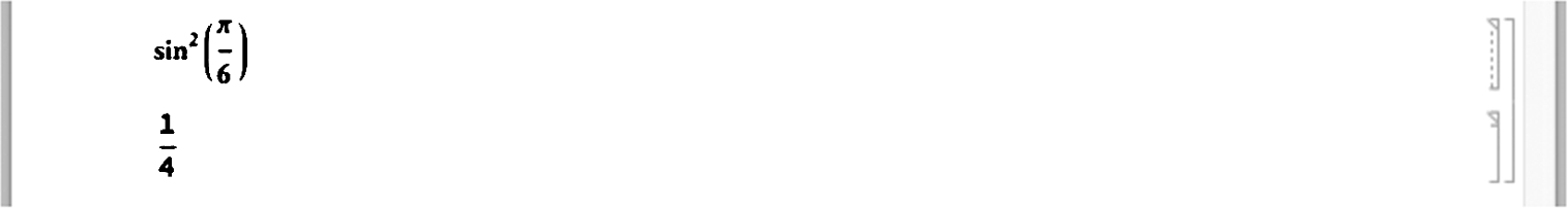
to be the product of the symbols sin2 and ![]() . However, using TraditionalForm we are able to evaluate
. However, using TraditionalForm we are able to evaluate ![]() with Mathematica using conventional mathematical notation.
with Mathematica using conventional mathematical notation.
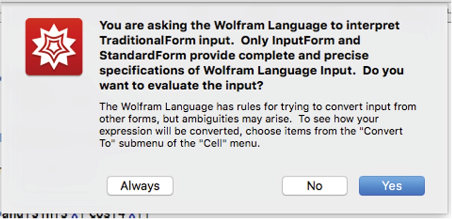
Be aware, however, that traditional mathematical notation does contain certain ambiguities and Mathematica may not return the result you expect if you enter input using TraditionalForm unless you are especially careful to follow the standard order of operations, as the following warning message indicates.
Example 2.7
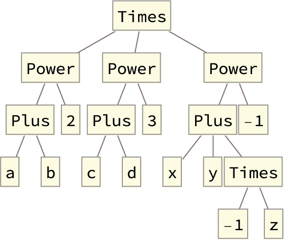
As stated, Mathematica follows the order of operations exactly. To see how Mathematica performs a calculation, TreeForm presents the sequence graphically.
For example, for the calculation ![]() , TreeForm gives us the results shown in Fig. 2.1.
, TreeForm gives us the results shown in Fig. 2.1.
![]()
2.2 Expressions and Functions: Elementary Algebra
2.2.1 Basic Algebraic Operations on Expressions
Expressions involving unknowns are entered in the same way as numbers. Mathematica performs standard algebraic operations on mathematical expressions. For example, the commands
1. Factor[expression] factors expression;
2. Expand[expression] multiplies expression;
3. Together[expression] writes expression as a single fraction; and
4. Simplify[expression] performs basic algebraic manipulations on expression and returns the simplest form it finds.
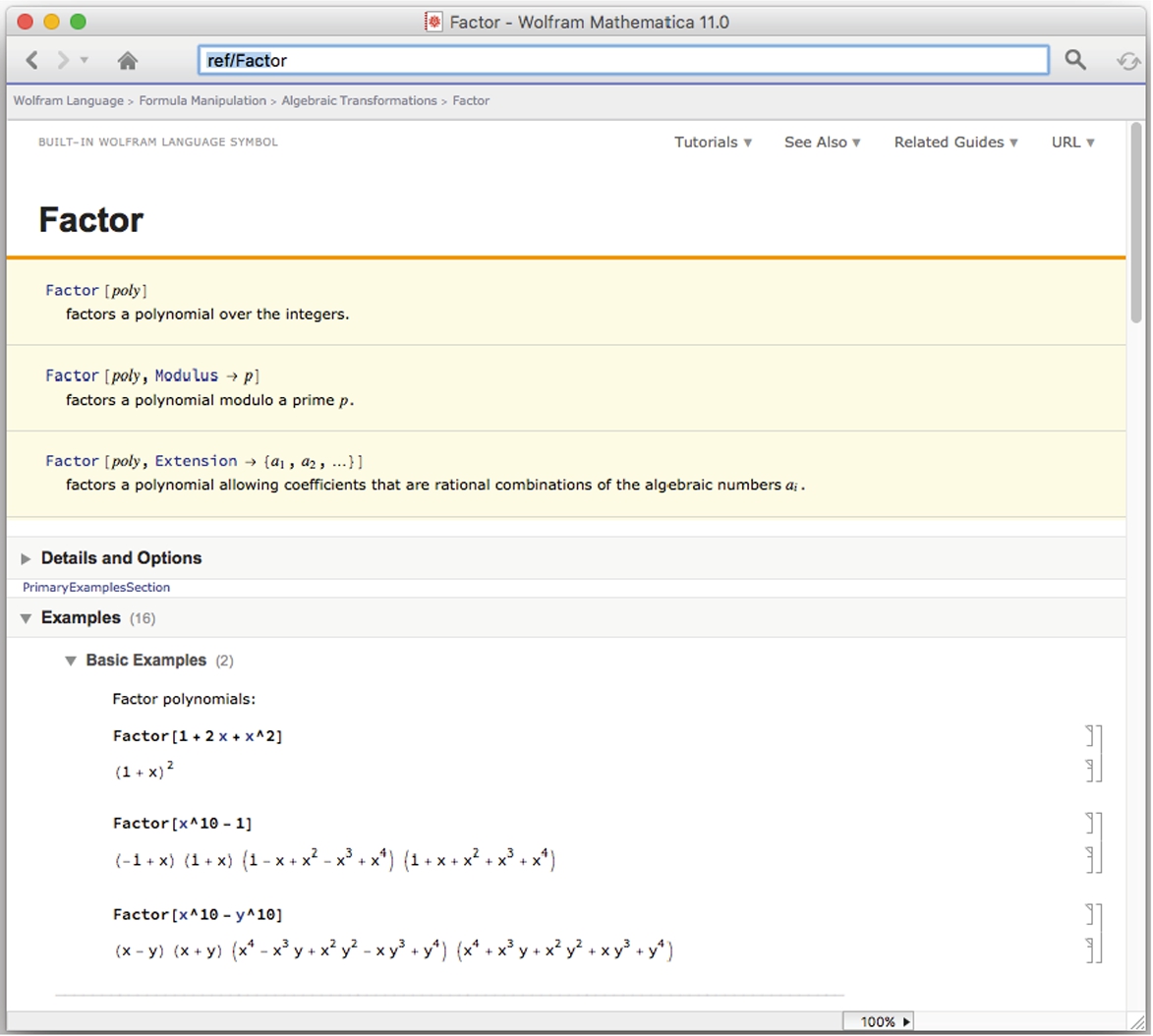
For basic information about any of these commands (or any other) enter ?command as we do here for Factor.
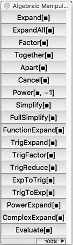
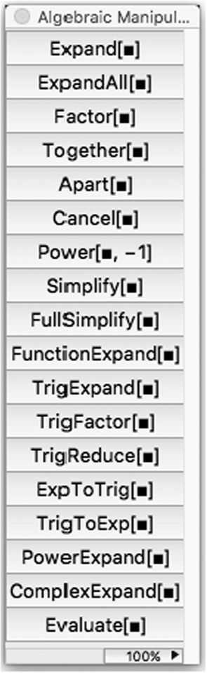
Many of the algebraic manipulation commands can be accessed from the AlgebraicManipulation palette.
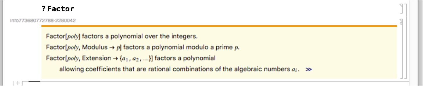
or access the Documentation Center as we do here for Factor.
When entering expressions, be sure to include a space or * between variables to denote multiplication to avoid any ambiguity or confusion. For example, Mathematica interprets 4x to be the product of x and 4. On the other hand, Mathematica interprets x4 to be a new symbol with the name “x4.” Similarly, xy is interpreted as a symbol with the name “xy” while x y and x*y are interpreted as the product of x and y, xy.
Example 2.8
(a) Factor the polynomial ![]() . (b) Expand the expression
. (b) Expand the expression ![]() . (c) Write the sum
. (c) Write the sum ![]() as a single fraction.
as a single fraction.
Solution
The result obtained with Factor indicates that ![]() . When typing the command, be sure to include a space, or *, between the x and y terms to denote multiplication. xy represents an expression while x y or x*y denotes x multiplied by y.
. When typing the command, be sure to include a space, or *, between the x and y terms to denote multiplication. xy represents an expression while x y or x*y denotes x multiplied by y.
![]()
![]()
We use Expand to compute the product ![]() and Together to express
and Together to express ![]() as a single fraction.
as a single fraction.
![]()
![]()
![]()
![]() □
□
To factor an expression like ![]() , use Factor with the Extension option.
, use Factor with the Extension option.
Factor[x̂2-3] returns ![]() .
.
![]()
![]()
Similarly, use Factor with the Extension option to factor expressions like ![]() .
.
![]()
![]()
![]()
![]()
Mathematica does not automatically simplify ![]() , to the expression x
, to the expression x
![]()
![]()
because without restrictions on x, ![]() . The command PowerExpand[expression] simplifies expression assuming that all variables are positive. Alternatively, you can use Assumptions to tell Mathematica to assume that
. The command PowerExpand[expression] simplifies expression assuming that all variables are positive. Alternatively, you can use Assumptions to tell Mathematica to assume that ![]() or to assume that
or to assume that ![]() .
.
![]()
x
![]()
−x
Alternatively, PowerExpand will automatically make “appropriate” assumptions when simplifying expressions.
![]()
x
Thus, entering
![]()
![]()
returns ![]() but entering
but entering
![]()
![]()
![]()
![]()
![]()
returns ![]() . However, if
. However, if ![]() and
and ![]() ,
, ![]() .
.
![]()
![]()
![]()
In general, a space is not needed between a number and a symbol to denote multiplication when a symbol follows a number. That is, 3dog means “3 times variable dog; dog3 is a variable with name dog3. Mathematica interprets 3 dog, dog*3, and dog 3 as “3 times variable dog. However, when multiplying two variables, either include a space or * between the variables.
1. cat dog means “variable cat times variable dog.”
2. cat*dog means “variable cat times variable dog.”
3. But, catdog is interpreted as a variable catdog.
The command Apart[expression] computes the partial fraction decomposition of expression; Cancel[expression] factors the numerator and denominator of expression then reduces expression to lowest terms.
Example 2.9
(a) Determine the partial fraction decomposition of ![]() . (b) Simplify
. (b) Simplify ![]() .
.
Solution
Apart is used to see that ![]() . Then, Cancel is used to find that
. Then, Cancel is used to find that ![]() . In this calculation, we have assumed that
. In this calculation, we have assumed that ![]() , an assumption made by Cancel but not by Simplify.
, an assumption made by Cancel but not by Simplify.
![]()
![]()
![]()
![]() □
□
In addition, Mathematica has several built-in functions for manipulating parts of fractions.
1. Numerator[fraction] yields the numerator of fraction.
2. ExpandNumerator[fraction] expands the numerator of fraction.
3. Denominator[fraction] yields the denominator of fraction.
4. ExpandDenominator[fraction] expands the denominator of fraction.
Example 2.10
Given ![]() , (a) factor both the numerator and denominator; (b) reduce
, (a) factor both the numerator and denominator; (b) reduce ![]() to lowest terms; and (c) find the partial fraction decomposition of
to lowest terms; and (c) find the partial fraction decomposition of ![]() .
.
Solution
The numerator of ![]() is extracted with Numerator. We then use Factor together with %, which is used to refer to the most recent output, to factor the result of executing the Numerator command.
is extracted with Numerator. We then use Factor together with %, which is used to refer to the most recent output, to factor the result of executing the Numerator command.
![]()
![]()
![]()
![]()
Similarly, we use Denominator to extract the denominator of the fraction. Again, Factor together with % is used to factor the previous result, which corresponds to the denominator of the fraction.
![]()
![]()
![]()
![]()
Cancel is used to reduce the fraction to lowest terms.
![]()
![]()
Finally, Apart is used to find its partial fraction decomposition.
![]()
![]() □
□
You can also take advantage of the AlgebraicManipulation palette, which is accessed by going to Palettes under the Mathematica menu, followed by AlgebraicManipulation, to evaluate expressions.
Example 2.11
Simplify ![]() .
.
Solution
First, we type the expression.
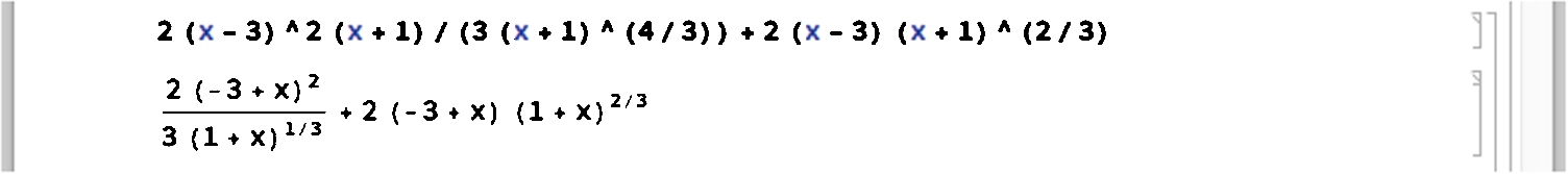
Then, select the expression.
![]()
Move the cursor to the palette and click on Simplify. Mathematica simplifies the expression.
![]() □
□
2.2.2 Naming and Evaluating Expressions
In Mathematica, objects can be named. Naming objects is convenient: we can avoid typing the same mathematical expression repeatedly (as we did in Example 2.10) and named expressions can be referenced throughout a notebook or Mathematica session. Every Mathematica object can be named – expressions, functions, graphics, and so on can be named with Mathematica. Objects are named by using a single equals sign (=).
Because every built-in Mathematica function begins with a capital letter, we adopt the convention that every mathematical object we name in this text will begin with a lowercase letter. Consequently, we will be certain to avoid any possible ambiguity with any built-in Mathematica objects.
With Mathematica 11, the default option is to display known objects in black and unknown objects in blue. Thus, in the following screen shot,
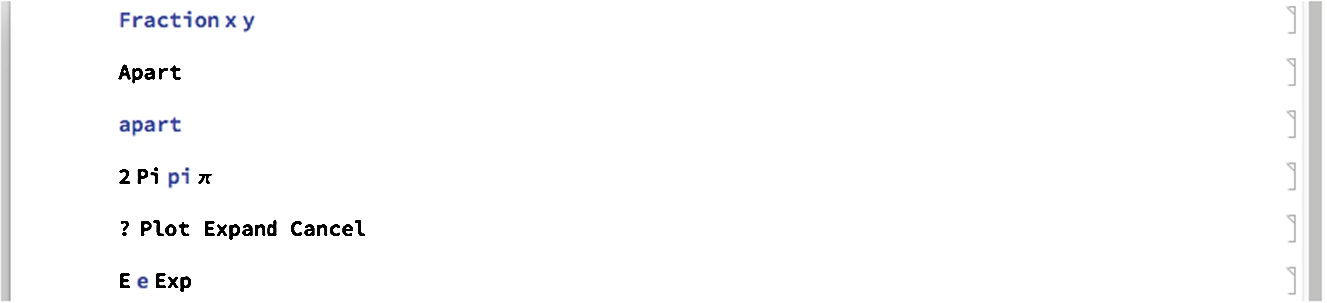
Fraction, x, y, apart, pi, and e are in blue; Apart, 2, Pi, π, ?, Plot, Expand, Cancel, Exp, and E are in black.
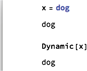
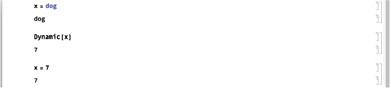
To automatically update named variables, Dynamic[x] returns the current value of x.
Thus, Dynamic[x] returns dog.
However, when we enter ![]() afterwards, Dynamic[x] is automatically updated to the new value of x.
afterwards, Dynamic[x] is automatically updated to the new value of x.
Expressions are easily evaluated using ReplaceAll, which is abbreviated with /. and obtained by typing a backslash (/) followed by a period (.), together with Rule, which is abbreviated with -> and obtained by typing a dash (minus sign) (-) followed by a greater than sign (>). For example, entering the command
x^2 /. x->3
returns the value of the expression ![]() if
if ![]() . Note, however, this does not assign the symbol x the value 3: entering x=3 assigns x the value 3.
. Note, however, this does not assign the symbol x the value 3: entering x=3 assigns x the value 3.
Example 2.12
Evaluate ![]() if
if ![]() ,
, ![]() , and
, and ![]() .
.
Solution
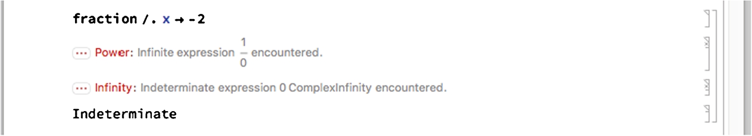
To avoid retyping ![]() , we define fraction to be
, we define fraction to be ![]() .
.
![]()
![]()
![]()
/. is used to evaluate fraction if ![]() and then if
and then if ![]() .
.
![]()
![]()
![]()
![]()
When we try to replace each x in fraction by 2, we see that the result is undefined: division by 0 is always undefined.
However, when we use Cancel to first simplify and then use ReplaceAll to evaluate,
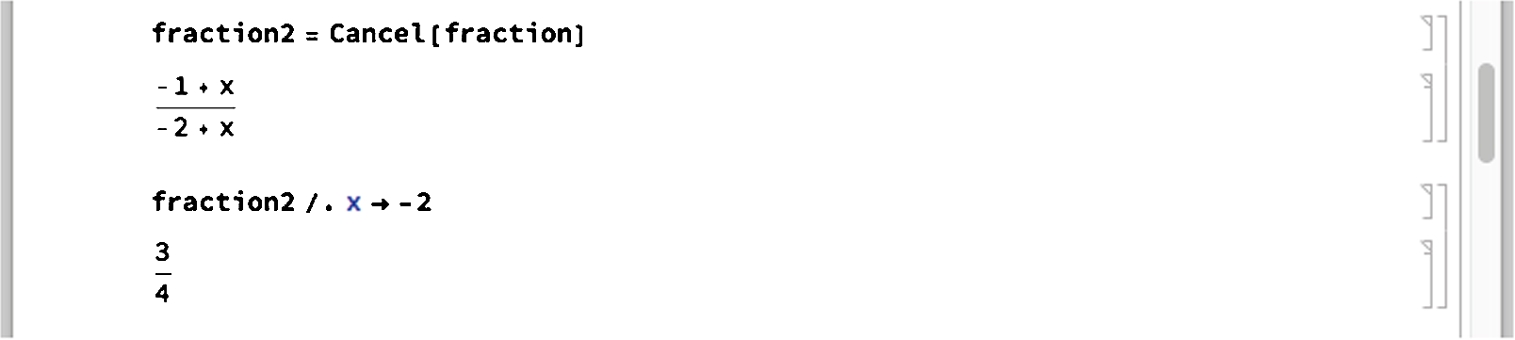
we see that the result is 3/4. The result indicates that ![]() . We confirm this result with Limit.
. We confirm this result with Limit.
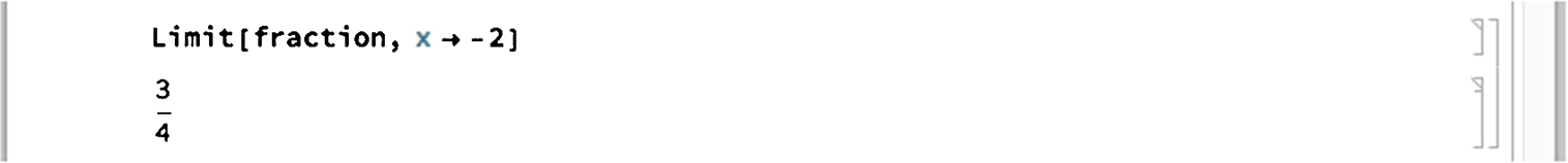
Generally, Limit[f[x],x->a] attempts to compute ![]() . The Limit function is discussed in more detail in the next chapter. □
. The Limit function is discussed in more detail in the next chapter. □
2.2.3 Defining and Evaluating Functions
It is important to remember that functions, expressions, and graphics can be named anything that is not the name of a built-in Mathematica function or command. As previously indicated, every built-in Mathematica object begins with a capital letter so every user-defined function, expression, or other object in this text will be assigned a name using lowercase letters, exclusively. This way, the possibility of conflicting with a built-in Mathematica command or function is completely eliminated. Because definitions of functions and names of objects are frequently modified, we introduce the command Clear. Clear[expression] clears all definitions of expression, if any. You can see if a particular symbol has a definition by entering ?symbol.
In Mathematica, an elementary function of a single variable, ![]()
![]() , is typically defined using the form
, is typically defined using the form
f[x_]=expression in x or f[x_]:=expression in x.
Notice that when you first define a function, you must always enclose the argument in square brackets ([...]) and place an underline (or blank) “_” after the argument on the left-hand side of the equals sign in the definition of the function.
Example 2.13
Entering
![]()
![]()
defines and computes ![]() . Entering
. Entering
![]()
![]()
computes ![]() . Entering
. Entering
![]()
![]()
computes ![]() . Entering
. Entering
![]()
![]()
computes ![]() . Entering
. Entering
![]()
![]()
computes and simplifies ![]() and names the result n1. Entering
and names the result n1. Entering
![]()
![]()
evaluates n1 if ![]() . Entering
. Entering
![]()
![]()
computes and simplifies ![]() and names the result n2. Entering
and names the result n2. Entering
![]()
![]()
evaluates n2 if ![]() .
.
Often, you will need to evaluate a function for the values in a list,
Once ![]() has been defined, Map[f,list] returns the list
has been defined, Map[f,list] returns the list
Also,
1. Table[f[n],{n,n1,n2}] returns the list
2. Table[(n,f[n]),{n,n1,n2}] returns the list of ordered pairs
Example 2.14
Entering
![]()
![]()
![]()
![]()
2
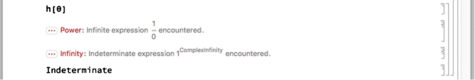
defines ![]() and then computes
and then computes ![]() . Because division by 0 is always undefined,
. Because division by 0 is always undefined, ![]() is undefined.
is undefined.
However, ![]() is defined for all
is defined for all ![]() . In the following, we use RandomReal together with Table to generate 6 random numbers “close” to 0 and name the resulting list t1. Because we are using RandomReal, your results will almost certainly differ from those here.
. In the following, we use RandomReal together with Table to generate 6 random numbers “close” to 0 and name the resulting list t1. Because we are using RandomReal, your results will almost certainly differ from those here.
![]()
![]()
We then use Map to compute ![]() for each of the values in the list t1.
for each of the values in the list t1.
From the result, we might correctly deduce that ![]() . We can compute the limit with the Limit function, which will be discussed in more detail in Chapter 3. For now, we remark that Limit[f[x],x->a] attempts to compute
. We can compute the limit with the Limit function, which will be discussed in more detail in Chapter 3. For now, we remark that Limit[f[x],x->a] attempts to compute ![]() .
.
![]()
e
In each of these cases, do not forget to include the “blank” (or underline) (_) on the left-hand side of the equals sign and right bracket in the definition of each function. Remember to always include arguments of functions in square brackets.
Example 2.15
Entering
![]()
![]()
![]()
![]()
defines the recursively-defined function defined by ![]() ,
, ![]() , and
, and ![]() . For example,
. For example, ![]() ;
; ![]() . We use Table to create a list of ordered pairs
. We use Table to create a list of ordered pairs ![]() for
for ![]() .
.
The ![]() we have defined here return the Fibonacci number
we have defined here return the Fibonacci number ![]() . Fibonacci[n] also returns the nth Fibonacci number.
. Fibonacci[n] also returns the nth Fibonacci number.
![]()
![]()
In the preceding examples, the functions were defined using each of the forms f[x_]:=... and f[x_]=.... As a practical matter, when defining “routine” functions with domains consisting of sets of real numbers and ranges consisting of sets of real numbers, either form can be used. Defining a function using the form f[x_]=... instructs Mathematica to define f and then compute and return f[x] (immediate assignment); defining a function using the form f[x_]:=... instructs Mathematica to define f. In this case, f[x] is not computed and, thus, Mathematica returns no output (delayed assignment). The form f[x_]:=... should be used when Mathematica cannot evaluate f[x] unless x is a particular value, as with recursively-defined functions or piecewise-defined functions which we will discuss shortly.
Generally, if attempting to define a function using the form f[x_]=... produces one or more error messages, use the form f[x_]:=... instead.
To define piecewise-defined functions, we usually use Condition (/;) as illustrated in the following example. In simple situations we take advantage of Piecewise.
Example 2.16
Entering
![]()
![]()
defines ![]() for
for ![]() . Entering
. Entering
![]()
0
is evaluated because ![]() . However, both of the following commands are returned unevaluated. In the first case, −1 is not greater than 0 (
. However, both of the following commands are returned unevaluated. In the first case, −1 is not greater than 0 (![]() is not defined for
is not defined for ![]() ). In the second case, Mathematica does not know the value of a so it cannot determine if it is or is not greater than 0.
). In the second case, Mathematica does not know the value of a so it cannot determine if it is or is not greater than 0.
![]()
![]()
![]()
![]()
Entering
![]()
defines ![]() for
for ![]() . Now, the domain of
. Now, the domain of ![]() is all real numbers. That is, we have defined the piecewise-defined function
is all real numbers. That is, we have defined the piecewise-defined function
We can now evaluate ![]() for any real number t.
for any real number t.
![]()
1
![]()
0
![]()
10
However, ![]() still returns unevaluated because Mathematica does not know if
still returns unevaluated because Mathematica does not know if ![]() or if
or if ![]() .
.
![]()
![]()
Recursively-defined functions are handled in the same way. The following example shows how to define a periodic function.
Example 2.17
Entering
![]()
![]()
![]()
![]()
![]()
defines the recursively-defined function ![]() . For
. For ![]() ,
, ![]() is defined by
is defined by
For ![]() ,
, ![]() . Entering
. Entering
![]()
1
computes ![]() . We use Table to create a list of ordered pairs
. We use Table to create a list of ordered pairs ![]() for 25 equally spaced values of x between 0 and 6.
for 25 equally spaced values of x between 0 and 6.
![]()
![]()
![]()
![]()
![]()
We will discuss additional ways to define, manipulate, and evaluate functions as needed. However, Mathematica's extensive programming language allows a great deal of flexibility in defining functions, many of which are beyond the scope of this text. These powerful techniques are discussed in detail in texts like Wellin's Programming with Mathematica: An Introduction [18], Gray's Mastering Mathematica: Programming Methods and Applications [9], Wellin's Essentials of Programming in Mathematica [19] and Maeder's The Mathematica Programmer II and Programming in Mathematica [12,13].
2.3 Graphing Functions, Expressions, and Equations
One of the best features of Mathematica is its graphics capabilities. In this section, we discuss methods of graphing functions, expressions, and equations and several of the options available to help graph functions.
2.3.1 Functions of a Single Variable
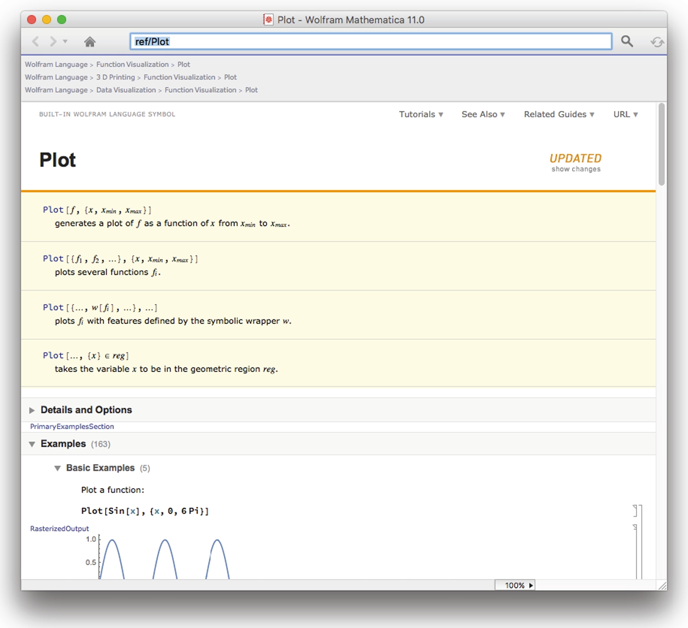
The commands
Plot[f[x],{x,a,b}] and Plot[f[x],{x,a,x1,x2,...,xn,b}]
graph the function ![]() on the intervals
on the intervals ![]() and
and ![]() , respectively. Mathematica returns information about the basic syntax of the Plot command with ?Plot or use the Documentation Center to obtain detailed information regarding Plot.
, respectively. Mathematica returns information about the basic syntax of the Plot command with ?Plot or use the Documentation Center to obtain detailed information regarding Plot.
Remember that every Mathematica object can be assigned a name, including graphics. Use Show to combine graphics together. Show[p1,p2,...,pn] displays the graphics p1, p2, ..., pn together. Show[GraphicsRow[{p1,p2,...,pn}]] displays the graphics p1, p2, ..., pn in a row. Show[GraphicsColumn[{p1,p2,...,pn}]] displays the graphics p1, p2, ..., pn in a column.
Show[GraphicsGrid[{{p11,p12,...,p1m},{p21,p22,...,p2m},...,
    {pn1,pn2,...,pnm}}]]
displays the graphics p11, pp12, ..., pnm in an n-row by m-column array.
Example 2.18
Graph ![]() and
and ![]() for
for ![]() .
.
Solution
Entering
![]()
graphs ![]() for
for ![]() and names the result p1. The plot is shown in Fig. 2.2 (a). With
and names the result p1. The plot is shown in Fig. 2.2 (a). With
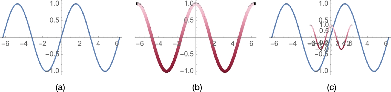
 for −2π ⩽ x ⩽ 2π. (b) A “reddish” plot of
  for −2π ⩽ x ⩽ 2π. (c) Combining two graphics with Epilog and Inset.
![]()
![]()
![]()
we create a slightly thicker plot of ![]() and shade the plot using the ValentineTones color gradient. See Fig. 2.2 (b).
and shade the plot using the ValentineTones color gradient. See Fig. 2.2 (b).
Show[p1,p2,...,pn] shows the graphics p1, ..., pn. You can also use Show to rerender graphics. Using Show with the Epilog option together with Inset, we place a small version of the cosine plot in the sine plot. See Fig. 2.2 (c).
![]()
![]()
Multiple graphics can be shown in rows, columns, or grids using GraphicsRow (to display several graphics as a row), GraphicsColumn (to display several graphics as a column) or GraphicsGrid (to display several graphics as a grid, array or matrix), respectively. Thus,
![]()
generates Fig. 2.2.
A different way of approaching the problem would be to graph the two functions to scale and then show them together. Include a semi-colon (;) at the end of a command to suppress the result. In the following, we graph ![]() in blue and
in blue and ![]() in red, naming the plots p1 and p2 respectively. Neither is displayed because we include a semi-colon at the end of each command. We then combine the graphics with Show. The result is shown to scale because the option AspectRatio->Automatic is included in the Show command (see Fig. 2.3).
in red, naming the plots p1 and p2 respectively. Neither is displayed because we include a semi-colon at the end of each command. We then combine the graphics with Show. The result is shown to scale because the option AspectRatio->Automatic is included in the Show command (see Fig. 2.3).
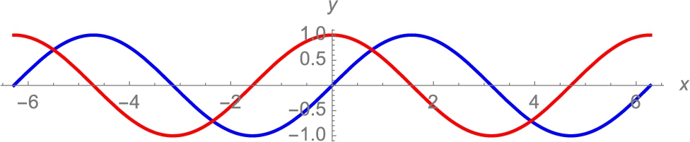 in blue and in red graphed to scale on the interval [−2π,2π]. (For interpretation of the colors in this figure, the reader is referred to the web version of this chapter.)
![]()
![]()
![]()
![]()
![]() □
□
Be careful when graphing functions with discontinuities. Often Mathematica will catch discontinuities. In other cases, it doesn't and you might need to use the Exclusions option to generate a more accurate plot.
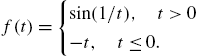
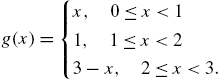
Example 2.19
Graph ![]() for
for ![]() where
where ![]() for
for ![]() and
and ![]() for
for ![]() .
.
Solution
After defining ![]() ,
,
![]()
![]()
![]()
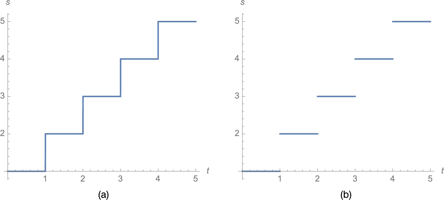
we use Plot to graph ![]() for
for ![]() in Fig. 2.4 (a).
in Fig. 2.4 (a).
![]()
![]()
Of course, Fig. 2.4 (a) is not completely precise: vertical lines are never the graphs of functions. In this case, discontinuities occur at ![]() , and 5. If we were to redraw the figure by hand, we would erase the vertical line segments, and then for emphasis place open dots at
, and 5. If we were to redraw the figure by hand, we would erase the vertical line segments, and then for emphasis place open dots at ![]() ,
, ![]() ,
, ![]() ,
, ![]() , and
, and ![]() and then closed dots at
and then closed dots at ![]() ,
, ![]() ,
, ![]() ,
, ![]() , and
, and ![]() . In cases like this where Plot does not automatically detect discontinuities you can specify them with Exclusions. See Fig. 2.4 (b).
. In cases like this where Plot does not automatically detect discontinuities you can specify them with Exclusions. See Fig. 2.4 (b).
![]()
![]()
![]()
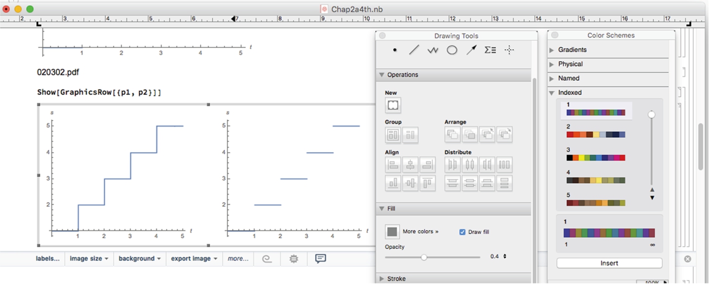
To fine-tune graphics, use the Drawing Tools and Graphics Inspector palettes, which are accessed under Graphics in the menu.
□
Entering Options[Plot] lists all Plot options and their default values. The most frequently used options include PlotStyle, DisplayFunction, AspectRatio, PlotRange, PlotLabel, and AxesLabel.
1. PlotStyle controls the color and thickness of a plot. PlotStyle-> GrayLevel[w], where ![]() instructs Mathematica to generate the plot in GrayLevel[w]. GrayLevel[0] corresponds to black and GrayLevel[1] corresponds to white. Color plots can be generated using RGBColor. RGBColor[1,0,0] corresponds to red, RGBColor[0,1,0] corresponds to green, and RGBColor[0,0,1] corresponds to blue. You can also use any of the named colors listed on the Color Schemes palette. If you prefer CMYK color coding, use CMYKColor[c,m,y,k] to help achieve the desired effects in your graphics.
instructs Mathematica to generate the plot in GrayLevel[w]. GrayLevel[0] corresponds to black and GrayLevel[1] corresponds to white. Color plots can be generated using RGBColor. RGBColor[1,0,0] corresponds to red, RGBColor[0,1,0] corresponds to green, and RGBColor[0,0,1] corresponds to blue. You can also use any of the named colors listed on the Color Schemes palette. If you prefer CMYK color coding, use CMYKColor[c,m,y,k] to help achieve the desired effects in your graphics.

PlotStyle->Dashing[{a1,a2,...,an}] indicates that successive segments be dashed with repeating lengths of ![]() ,
, ![]() , …,
, …, ![]() . The thickness of the plot is controlled with PlotStyle->Thickness[w], where w is the fraction of the total width of the graphic. For a single plot, the PlotStyle options are combined with PlotStyle->{{option1, option2, ... , optionn}].
. The thickness of the plot is controlled with PlotStyle->Thickness[w], where w is the fraction of the total width of the graphic. For a single plot, the PlotStyle options are combined with PlotStyle->{{option1, option2, ... , optionn}].
2. A plot is not displayed when the option DisplayFunction-> Identity is included or when a semi-colon (;) is included at the end of the command. Including the option DisplayFunction->$ DisplayFunction in Show or Plot commands instructs Mathematica to display graphics.
3. The ratio of height to width of a plot is controlled by AspectRatio. The default is 1/GoldenRatio. Generally, a plot is drawn to scale when the option AspectRatio-> Automatic is included in the Plot or Show command.
4. PlotRange controls the horizontal and vertical axes. PlotRange->{c,d} specifies that the vertical axis displayed corresponds to the interval ![]() while PlotRange->{{a,b}, {c,d}} specifes that the horizontal axis displayed corresponds to the interval
while PlotRange->{{a,b}, {c,d}} specifes that the horizontal axis displayed corresponds to the interval ![]() and that the vertical axis displayed corresponds to the interval
and that the vertical axis displayed corresponds to the interval ![]() .
.
5. PlotLabel->"titleofplot" labels the plot titleofplot.
6. AxesLabel->{"xaxislabel","yaxislabel"} labels the x-axis with xaxislabel and the y-axis with yaxislabel.
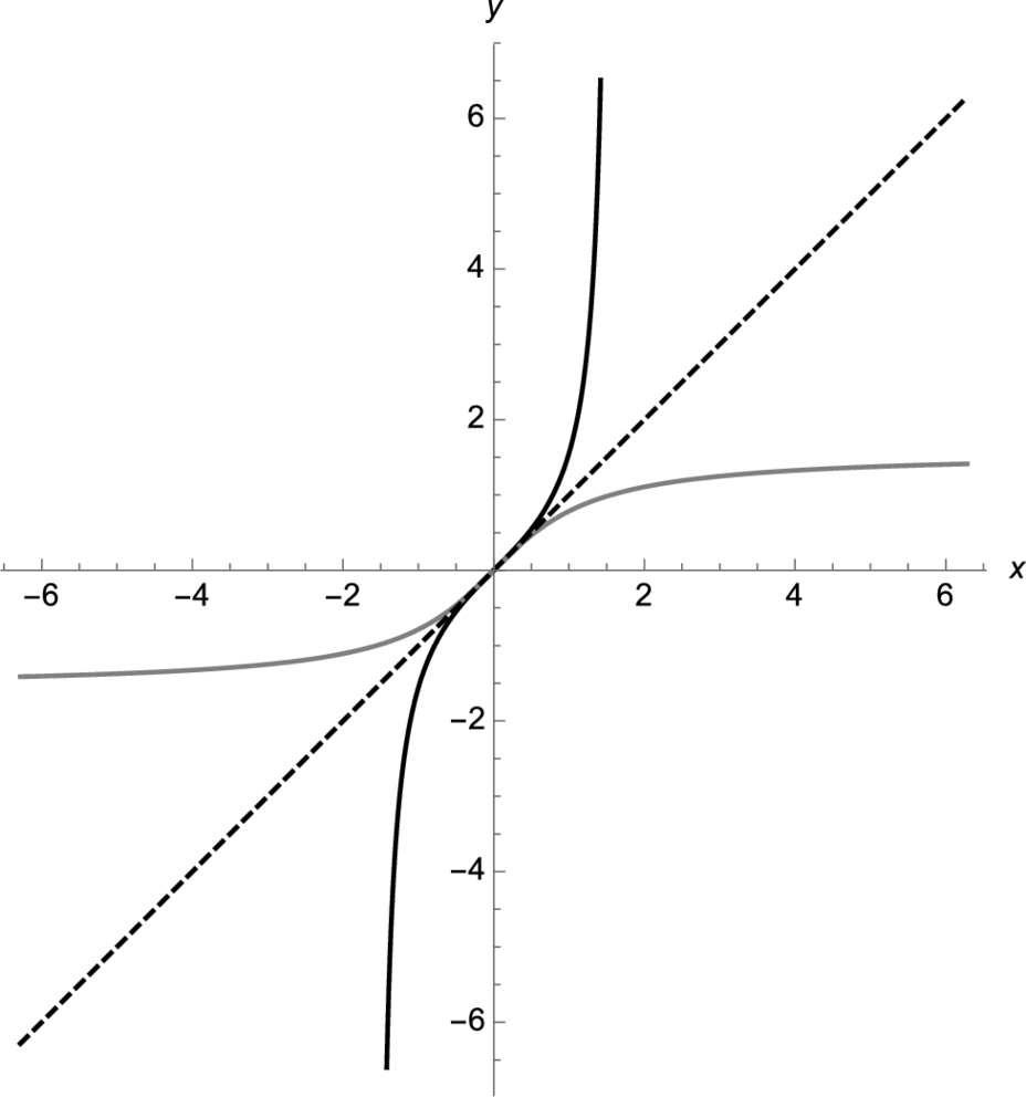
Example 2.20
Graph ![]() ,
, ![]() , and
, and ![]() together with their inverse functions.
together with their inverse functions.
Solution
In p2 and p3, we use Plot to graph ![]() and
and ![]() , respectively. Neither plot is displayed because we include a semi-colon at the end of the Plot commands. p1, p2, and p3 are displayed together with Show in Fig. 2.5 (a). The plot is shown to scale; the graph of
, respectively. Neither plot is displayed because we include a semi-colon at the end of the Plot commands. p1, p2, and p3 are displayed together with Show in Fig. 2.5 (a). The plot is shown to scale; the graph of ![]() is in black,
is in black, ![]() is in gray, and
is in gray, and ![]() is dashed.
is dashed.
 ,
,  , and y = x. (b) ,
  , and y = x.
![]()
![]()
![]()
![]()
![]()
![]()
![]()
![]()
The command Plot[{f1[x],f2[x],...,fn[x]},{x,a,b}] plots ![]() ,
, ![]() , …,
, …, ![]() together for
together for ![]() . Simple PlotStyle options are incorporated with
. Simple PlotStyle options are incorporated with
PlotStyle->{option1,option2,...,optionn
where optioni corresponds to the plot of ![]() . Multiple options are incorporated using
. Multiple options are incorporated using
PlotStyle->{{options1},{options2},...,{optionsn}}
where optionsi are the options corresponding to the plot of ![]() .
.
In the following, we use Plot to graph ![]() ,
, ![]() , and
, and ![]() together. The plot in Fig. 2.5 (b) is shown to scale; the graph of
together. The plot in Fig. 2.5 (b) is shown to scale; the graph of ![]() is in black,
is in black, ![]() is in gray, and
is in gray, and ![]() is dashed.
is dashed.
![]()
![]()
![]()
![]()
![]()
![]()
![]()
![]()
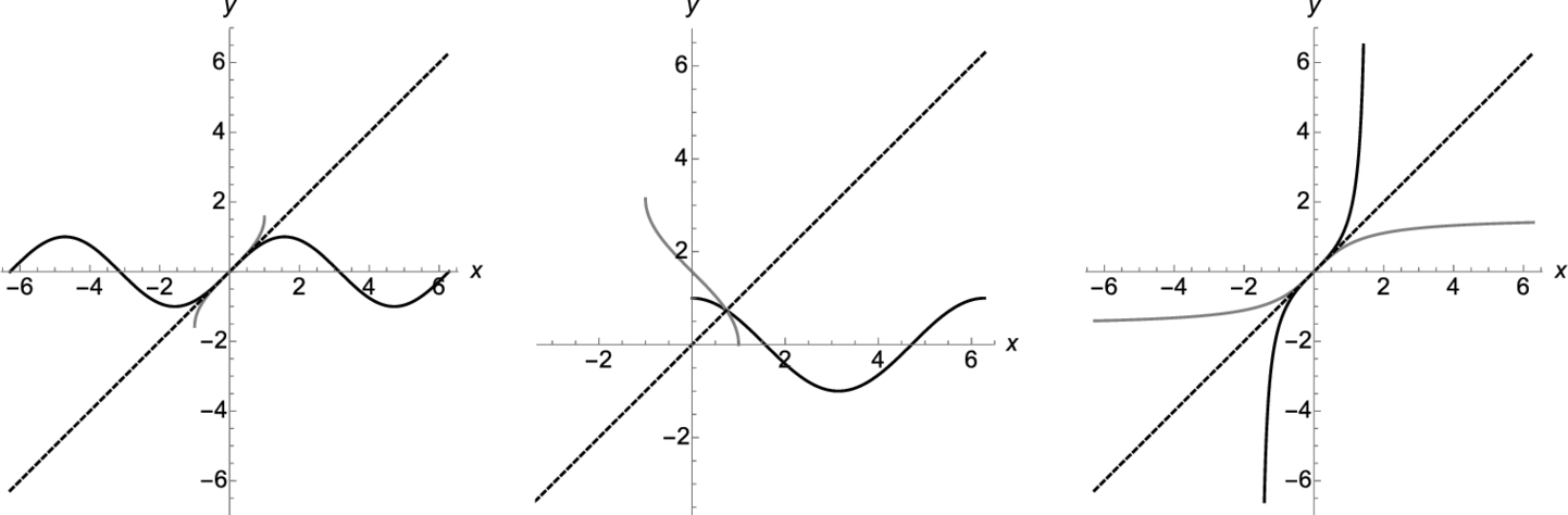
We use the same approach to graph ![]() ,
, ![]() , and
, and ![]() in Fig. 2.6.
in Fig. 2.6.
 ,
,  , and y = x.
![]()
![]()
![]()
![]()
![]()
![]()
![]()
![]()
Use Show together with GraphicsRow to display graphics in rectangular arrays. Entering
![]()
shows the three plots p2, p3, and t1c in a row as shown in Fig. 2.7. □
Example 2.21
Inverse Functions
![]() and
and ![]() are inverse functions if
are inverse functions if
If ![]() and
and ![]() are inverse functions, their graphs are symmetric about the line
are inverse functions, their graphs are symmetric about the line ![]() . The command
. The command
Composition[f1,f2,f3,...,fn,x]
computes the composition
For two functions ![]() and
and ![]() , it is usually easiest to compute the composition
, it is usually easiest to compute the composition ![]() with f[g[x]] or f[x]//g.
with f[g[x]] or f[x]//g.
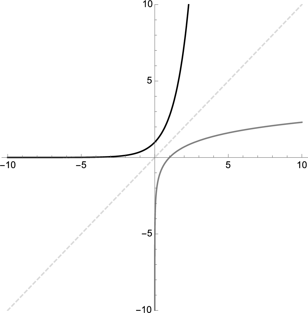
Show that
are inverse functions.
Solution
When using Mathematica, Exp[x] represents the function ![]() . Similarly, Log[x] represents the natural logarithm function,
. Similarly, Log[x] represents the natural logarithm function, ![]() .
.
After defining ![]() and
and ![]() ,
,
![]() and
and ![]() are not returned because a semi-colon is included at the end of each command.
are not returned because a semi-colon is included at the end of each command.
![]()
![]()
![]()
x
![]()
![]()
we compute and simplify the compositions ![]() and
and ![]() . Because both results simplify to
. Because both results simplify to ![]() ,
, ![]() and
and ![]() are inverse functions. Observe that Simplify does not automatically reduce
are inverse functions. Observe that Simplify does not automatically reduce ![]() . To do so, we use PowerExpand.
. To do so, we use PowerExpand.
![]()
x
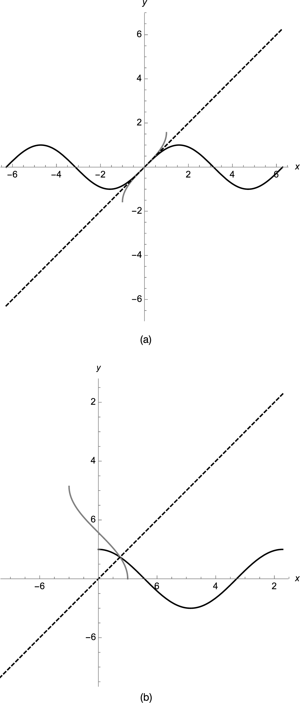
To see that the graphs of ![]() and
and ![]() are symmetric about the line
are symmetric about the line ![]() , we use Plot to graph
, we use Plot to graph ![]() ,
, ![]() , and
, and ![]() together in Fig. 2.8. Because Tooltip is being applied to the set of functions being plotted, you can identify each curve by sliding the cursor over the curve: when the cursor is placed over a curve, Mathematica displays its definition. In the Plot command, observe how we are able to graph all three functions,
together in Fig. 2.8. Because Tooltip is being applied to the set of functions being plotted, you can identify each curve by sliding the cursor over the curve: when the cursor is placed over a curve, Mathematica displays its definition. In the Plot command, observe how we are able to graph all three functions, ![]() ,
, ![]() , and
, and ![]() together as well as control how each graph is plotted using the PlotStyle option. The range (y-axis) displayed is controlled using the PlotRange option. The option AspectRatio->1 instructs Mathematica to display the axes in a
together as well as control how each graph is plotted using the PlotStyle option. The range (y-axis) displayed is controlled using the PlotRange option. The option AspectRatio->1 instructs Mathematica to display the axes in a ![]() (square) ratio. In this case, because the domains and ranges are the same, the resulting plot is drawn to scale. If the domains and ranges are not the same and you wish to have the plot displayed to scale, use the option AspectRatio->Automatic.
(square) ratio. In this case, because the domains and ranges are the same, the resulting plot is drawn to scale. If the domains and ranges are not the same and you wish to have the plot displayed to scale, use the option AspectRatio->Automatic.
 in gray, and y = x dashed in light gray.
![]()
![]()
![]()
In the plot, observe that the graphs of ![]() and
and ![]() are symmetric about the line
are symmetric about the line ![]() . The plot also illustrates that the domain and range of a function and its inverse are interchanged:
. The plot also illustrates that the domain and range of a function and its inverse are interchanged: ![]() has domain
has domain ![]() and range
and range ![]() ;
; ![]() has domain
has domain ![]() and range
and range ![]() . □
. □
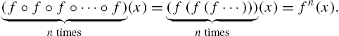
For repeated compositions of a function with itself, Nest[f,x,n] computes the composition
Example 2.22
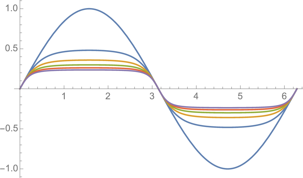
Graph ![]() ,
, ![]() ,
, ![]() ,
, ![]() ,
, ![]() , and
, and ![]() if
if ![]() for
for ![]() .
.
Solution
After defining ![]() ,
,
![]()
we graph ![]() in p1 with Plot
in p1 with Plot
![]()
and then illustrate the use of Nest by computing ![]() .
.
![]()
![]()
Next, we use Table together with Nest to create the list of functions
Because the resulting output is rather long, we include a semi-colon at the end of the Table command to suppress the resulting output.
Table[f[i],{i,a,b,istep}] computes ![]() for i values from a to b using increments of
for i values from a to b using increments of ![]() .
.
![]()
We then graph the functions in toplot on the interval ![]() with Plot, applying the Tooltip function to the list being plotted so they can easily be identified. Last, we use Show to display p1 and p2 together in Fig. 2.9.
with Plot, applying the Tooltip function to the list being plotted so they can easily be identified. Last, we use Show to display p1 and p2 together in Fig. 2.9.
![]()
![]()
In the plot, we see that repeatedly composing sine with itself has a flattening effect on ![]() . □
. □
When graphing functions involving odd roots, Mathematica's results may be surprising to the beginner. The key is to use the Surd function or remember that Mathematica follows the order of operations exactly and understand that without restrictions on x, ![]() .
.
Example 2.23
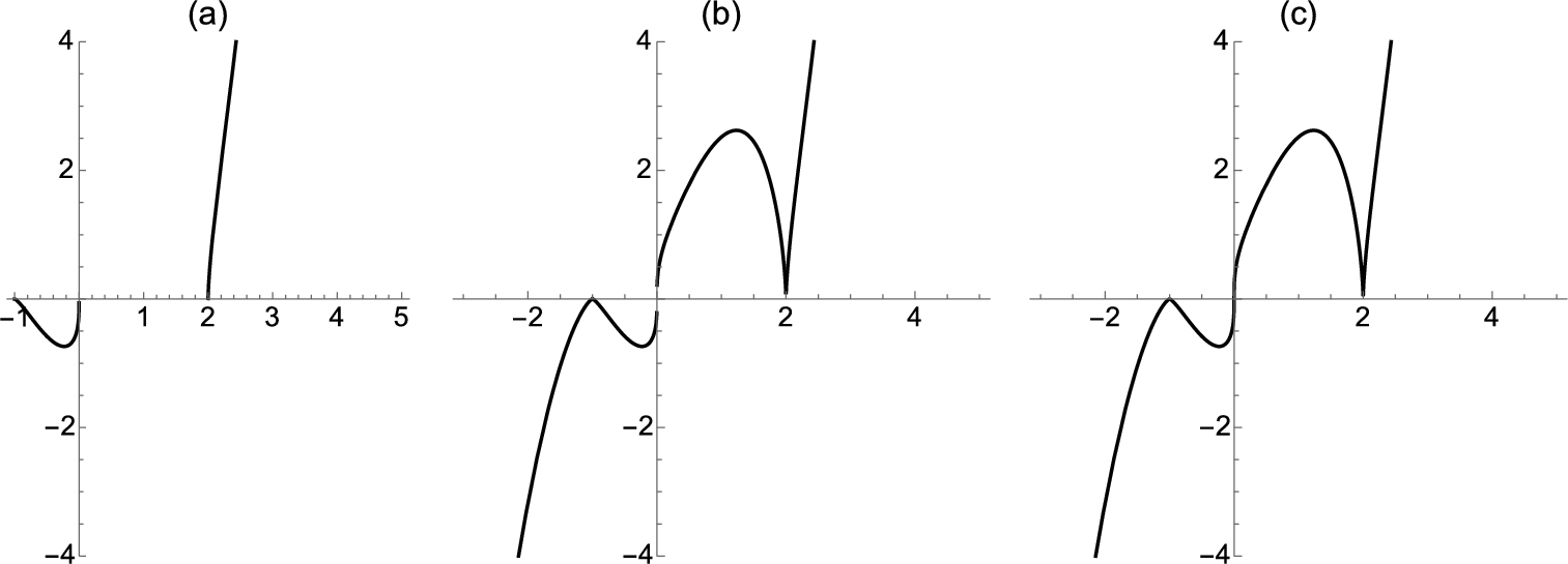
Graph ![]() .
.
Solution
Entering
![]()
![]()
![]()
![]()
does not produce the graph we expect (see Fig. 2.10 (a)) because many of us consider ![]() to be a real-valued function with domain
to be a real-valued function with domain ![]() . Generally, Mathematica does return a real number when computing the odd root of a negative number. For example,
. Generally, Mathematica does return a real number when computing the odd root of a negative number. For example, ![]() has three solutions
has three solutions
![]()
![]()
![]()
![]()
![]()
When computing an odd root of a negative number, Mathematica has many choices (as illustrated above) and chooses a root with positive imaginary part – the result is not a real number.
![]()
![]()
To obtain real values when computing odd roots of negative numbers, first let ![]() Sign[x] returns
Sign[x] returns ![]() . Then, for the reduced fraction
. Then, for the reduced fraction ![]() with m odd,
with m odd, ![]() . See Fig. 2.10 (b).
. See Fig. 2.10 (b).
![]()
![]()
![]()
Alternatively, use the Surd function to obtain the desired results. Surd[x,n] returns the real-valued nth root of x.
![]()
![]()
![]()
![]()
All three graphics are shown in Fig. 2.10 using Show together with GraphicsRow.
![]() □
□
The command
ListPlot[{{x1,y1},{x2,y2},...,{xn,yn}}]
plots the list of points ![]() . The size of the points in the resulting plot is controlled with the option PlotStyle->PointSize[w], where w is the fraction of the total width of the graphic. For two-dimensional graphics, the default value is 0.008. The command
. The size of the points in the resulting plot is controlled with the option PlotStyle->PointSize[w], where w is the fraction of the total width of the graphic. For two-dimensional graphics, the default value is 0.008. The command
ListPlot[{y1,y2,..,yn}]
plots the list of points ![]() . To connect successive points with line segments, use the command ListLinePlot.
. To connect successive points with line segments, use the command ListLinePlot.
ListLinePlot[{x1,y1},{x2,y2},...,{xn,yn}}]
connects the consecutive points ![]() ,
, ![]() , …,
, …, ![]() with line segments.
with line segments.
Solution
The “principal trigonometric values” are usually interpreted to mean the values of the functions ![]() and
and ![]() at the angles
at the angles ![]() ,
, ![]() ,
, ![]() ,
, ![]() ,
, ![]() ,
, ![]() ,
, ![]() ,
, ![]() , π,
, π, ![]() ,
, ![]() ,
, ![]() ,
, ![]() ,
, ![]() ,
, ![]() ,
, ![]() , and 2π.
, and 2π.
We begin by defining these points in prinvals. These points are then plotted in lp1 with ListPlot. We illustrate the use of the PlotStyle, AspectRatio, and PlotLabel options.
![]()
![]()
![]()
![]()
![]()
![]()
![]()
Next, we define prinlines to be a set of ordered pairs that will draw line segments between connected points. These lines are graphed by using Map to apply ListLinePlot to each ordered pair in prinlines. Generally, Map[f,list] applies the function f to each element of list. We use Show and illustrate the use of the AspectRatio and PlotLabel options to graph these line segments in lp2.
![]()
![]()
![]()
![]()
![]()
![]()
![]()
![]()
![]()
![]()
In lp3, we use Plot to graph the functions ![]() and
and ![]() . In the color version of this text, the CMYKColor code corresponds to a deep red. The graph is drawn to scale because we include the option AspectRatio->Automatic.
. In the color version of this text, the CMYKColor code corresponds to a deep red. The graph is drawn to scale because we include the option AspectRatio->Automatic.
![]()
![]()
![]()
Finally, we use Show to display all four graphics together in lp4.
![]()
The four images are displayed as a graphics grid using Show together with GraphicsGrid in Fig. 2.11.
![]() □
□
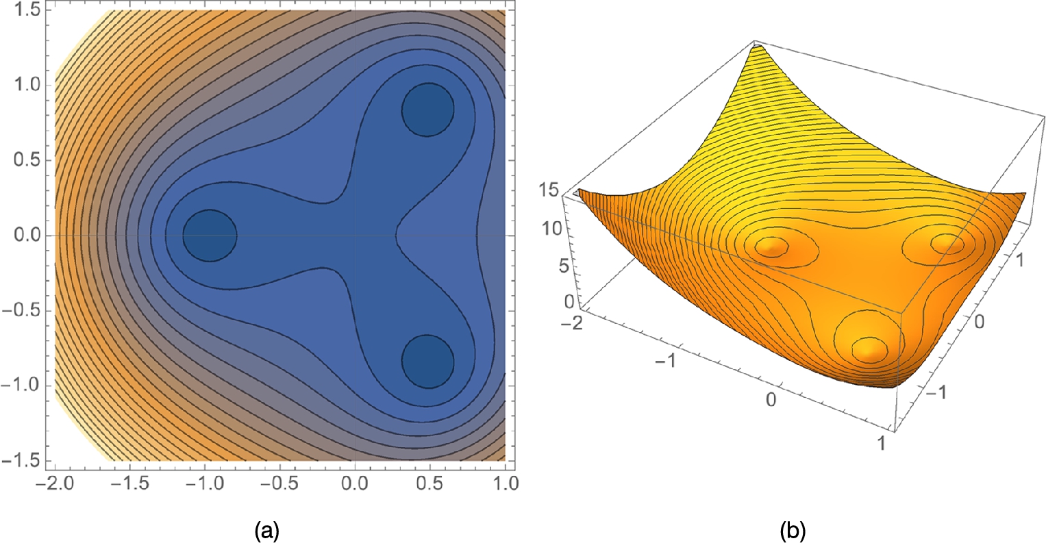
A comprehensive discussion of Mathematica's extensive graphics capabilities cannot be reasonably covered in a single section of a text so our approach is to address issues that might of interest or present a different point of view to the beginning user of Mathematica. In the previous example, we saw that ![]() has three solutions, two of which are complex. To visualize this graphically, observe that the zeros of
has three solutions, two of which are complex. To visualize this graphically, observe that the zeros of ![]() are the level curves of
are the level curves of ![]() (x, y real) corresponding to 0. In a plot of
(x, y real) corresponding to 0. In a plot of ![]() , the solutions are the zeros. Shortly we will discuss ContourPlot and Plot3D. For now, we remark that
, the solutions are the zeros. Shortly we will discuss ContourPlot and Plot3D. For now, we remark that
![]()
![]()
![]()
![]()
![]()
![]()
generates several level curves of ![]() (Fig. 2.12 (a)) and a 3-d plot of
(Fig. 2.12 (a)) and a 3-d plot of ![]() (Fig. 2.12 (b)) that help us see the zeros of the original equation. In the 3-d plot, note how we use the MeshFunctions option to generate contours on the 3-d plot.
(Fig. 2.12 (b)) that help us see the zeros of the original equation. In the 3-d plot, note how we use the MeshFunctions option to generate contours on the 3-d plot.
2.3.2 Parametric and Polar Plots in Two Dimensions
For parametrically defined functions, ![]() ,
, ![]() ,
, ![]() , use ParametricPlot. ParametricPlot[{x[t],y[t]},{t,a,b}] attempts to graph the parametrically defined functions
, use ParametricPlot. ParametricPlot[{x[t],y[t]},{t,a,b}] attempts to graph the parametrically defined functions ![]() ,
, ![]() ,
, ![]() .
.
To graph the polar function, ![]() , use PolarPlot.
, use PolarPlot.
PolarPlot[f[theta],{theta,alpha,beta}]
attempts to graph ![]() for
for ![]() .
.

Example 2.25
The Unit Circle
The unit circle is the set of points ![]() exactly 1 unit from the origin,
exactly 1 unit from the origin, ![]() , and, in rectangular coordinates, has equation
, and, in rectangular coordinates, has equation ![]() . The unit circle is the classic example of a relation that is neither a function of x nor a function of y. The top half of the unit circle is given by
. The unit circle is the classic example of a relation that is neither a function of x nor a function of y. The top half of the unit circle is given by ![]() and the bottom half is given by
and the bottom half is given by ![]() .
.
![]()
![]()
![]()
![]()
Each point ![]() on the unit circle is a function of the angle, t, that subtends the x-axis, which leads to a parametric representation of the unit circle,
on the unit circle is a function of the angle, t, that subtends the x-axis, which leads to a parametric representation of the unit circle, ![]() , which we graph with ParametricPlot.
, which we graph with ParametricPlot.
![]()
![]()
![]()
![]()
Using the change of variables ![]() and
and ![]() to convert from rectangular to polar coordinates, a polar equation for the unit circle is
to convert from rectangular to polar coordinates, a polar equation for the unit circle is ![]() . We use PolarPlot to graph
. We use PolarPlot to graph ![]() .
.
![]()
![]()
![]()
We display p1, p2, and p3 side-by-side using Show together with GraphicsRow in Fig. 2.13. Of course, they all look the same, just in different colors (or shades of gray if you are reading the printed version of this text).
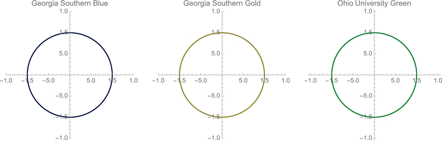
![]()
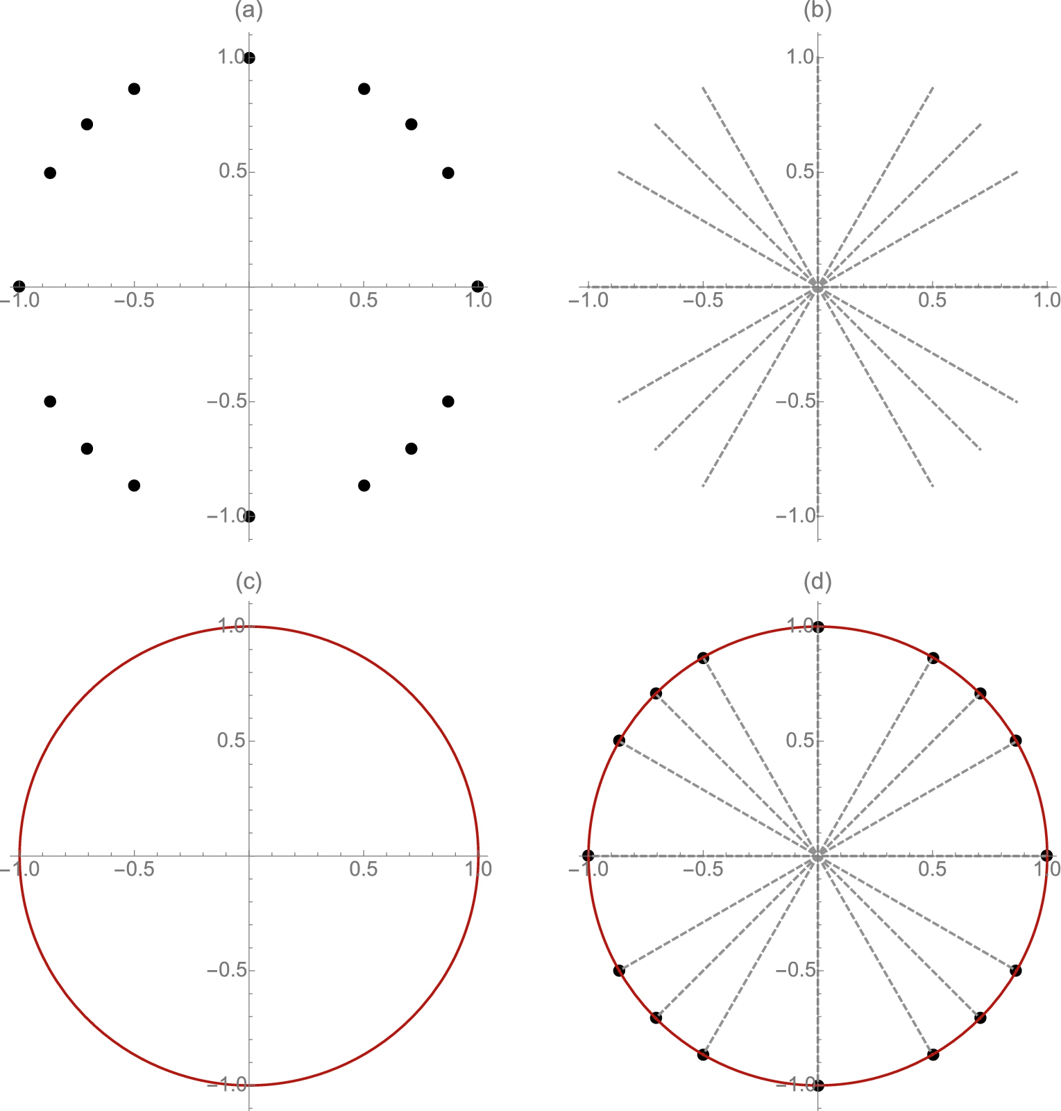
To illustrate several other features of Mathematica's extensive graphics capability, we elaborate on the example and construct a unit circle that can be used as a handout in a trigonometry, pre-calculus, or calculus class.
In p1, we graph the unit circle.
![]()
![]()
Next, we use ParametricPlot to connect the principal value points on the unit circle with line segments by observing that the parametric equations ![]() ,
, ![]() ,
, ![]() graphs a line segment connecting
graphs a line segment connecting ![]() and
and ![]() .
.
![]()
![]()
![]()
![]()
![]()
![]()
![]()
![]()
![]()
![]()
![]()
![]()
![]()
![]()
![]()
![]()
![]()
![]()
![]()
![]()
Next, we use the graphics primitive Text to label the principal values on the unit circle.

![]()
![]()
![]()
![]()
![]()
![]()
![]()
![]()
![]()
![]()
![]()
![]()
Our last step is to combine these graphics objects together and show them as a single image with Show.
![]()
![]()
In the following example, the equations of the parametrically defined functions involve integrals.
Remark 2.2
Topics from calculus are discussed in Chapter 3. For now, we state that Integrate[f[x],{x,a,b}] attempts to evaluate ![]() .
.
Rather than explicitly stating the color as in the previous example, we use gradients from the Color Scheme palette to adjust the colors in the resulting graphics (see Fig. 2.14).

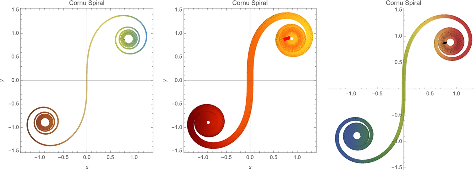
Example 2.26
Cornu Spiral
Solution
We begin by defining x and y. Notice that Mathematica can evaluate these integrals, even though the results are in terms of the FresnelS and FresnelC functions, which are defined in terms of integrals:

![]()
![]()
![]()
![]()
We use ParametricPlot to graph the Cornu spiral in Fig. 2.15. The option AspectRatio->Automatic instructs Mathematica to generate the plot to scale; PlotLabel->"Cornu spiral" labels the plot. Rather than explicitly stating the color, we use gradients from the Color Scheme palette to adjust the color of the plot.
![]()
![]()
![]()
![]()
![]()
![]()
![]()
![]()
![]()
![]()
![]()
![]()
We use Show together with GraphicsRow to display the three graphics together in Fig. 2.15.
![]() □
□
Observe that the graph of the polar equation ![]() ,
, ![]() is the same as the graph of the parametric equations
is the same as the graph of the parametric equations
so both ParametricPlot and PolarPlot can be used to graph polar equations.
Example 2.27
Graph (a) ![]() ,
, ![]() ; (b)
; (b) ![]() ,
, ![]() ; (c) (“The Butterfly”)
; (c) (“The Butterfly”) ![]() ,
, ![]() ; and (d) (“The Lituus”)
; and (d) (“The Lituus”) ![]() ,
, ![]() .
.
Solution
For (a) and (b) we use ParametricPlot. First define r and then use ParametricPlot to generate the graph of the polar curve. No graphics are displayed because we place a semi-colon at the end of each command. We illustrate the use of various options, particularly the PlotStyle and PlotLabel options in each.
![]()
![]()
![]()
![]()
![]()
![]()
For (b), we use the option PlotRange->{{-30,30},{-30,30}} to indicate that the range displayed on both the vertical and horizontal axes corresponds to the interval ![]() . To help assure that the resulting graphic appears “smooth”, we increase the number of points that Mathematica samples when generating the graph by including the option PlotPoints->200.
. To help assure that the resulting graphic appears “smooth”, we increase the number of points that Mathematica samples when generating the graph by including the option PlotPoints->200.
![]()
![]()
![]()
![]()
![]()
![]()
![]()
For (c) and (d), we use PolarPlot. Using standard mathematical notation, we know that ![]() . However, when defining r with Mathematica, be sure you use the form
. However, when defining r with Mathematica, be sure you use the form ![]() , not
, not ![]() , which Mathematica will not interpret in the way intended.
, which Mathematica will not interpret in the way intended.
![]()
![]()
![]()
![]()
![]()
![]()
![]()
![]()
![]()
![]()
![]()
Finally, we use Show together with GraphicsGrid to display all four graphs as a graphics array in Fig. 2.16. pp1 and pp2 are shown in the first row; pp3 and pp4 in the second.

![]() □
□
2.3.3 Three-Dimensional and Contour Plots; Graphing Equations
An elementary function of two variables, ![]() , is typically defined using the form
, is typically defined using the form
f[x_,y_]=expression in x and y.
For delayed evaluation, use f[x_,y_]:=... rather than f[x_,y_]=... (immediate evaluation). Once a function has been defined, a basic graph is generated with Plot3D:
Plot3D[f[x,y],{x,a,b},{y,c,d}]
graphs ![]() for
for ![]() and
and ![]() .
.
For details regarding Plot3D and its options enter ?Plot3D or ??Plot3D or access the Documentation Center to obtain information about the Plot3D command, as we do here.
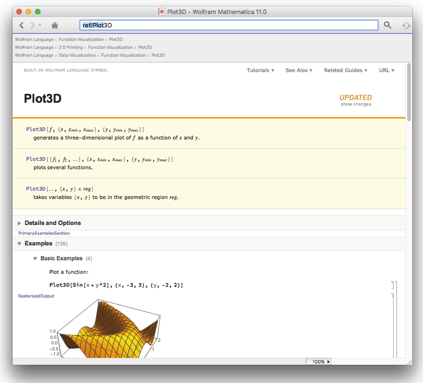
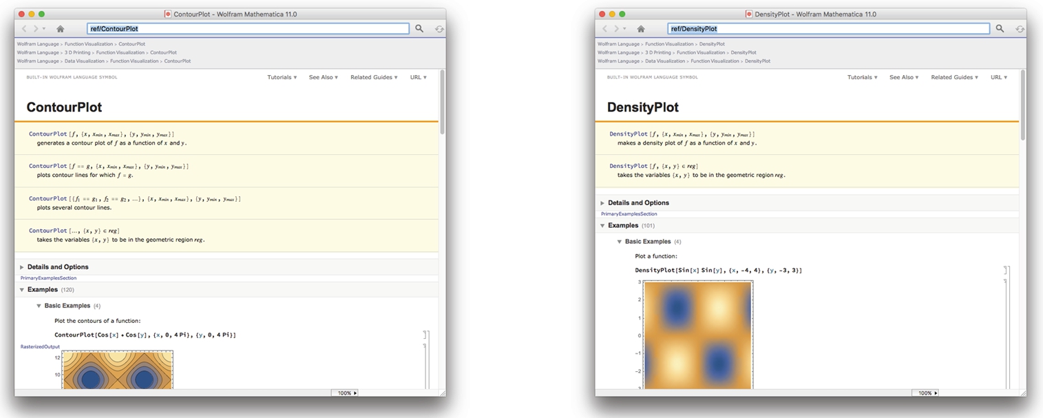
Graphs of several level curves of ![]() are generated with
are generated with
ContourPlot[f[x,y],{x,a,b},{y,c,d}].
A density plot of ![]() is generated with
is generated with
DensityPlot[f[x,y],{x,a,b},{y,c,d}].
For details regarding ContourPlot (DensityPlot) and its options enter ?ContourPlot (?DensityPlot) or ??ContourPlot (??DensityPlot) or access the Documentation Center.
Example 2.28
Let ![]() . (a) Calculate
. (a) Calculate ![]() . (b) Graph
. (b) Graph ![]() and several contour plots of
and several contour plots of ![]() on a region containing the origin,
on a region containing the origin, ![]() .
.
Solution
After defining ![]() , we evaluate
, we evaluate ![]() .
.
![]()
![]()
![]()
![]()
Next, we use Plot3D to graph ![]() for
for ![]() and
and ![]() in Fig. 2.17. We illustrate the use of the Axes, Boxed, PlotPoints, MeshFunctions, PlotStyle, and ColorFunction options.
in Fig. 2.17. We illustrate the use of the Axes, Boxed, PlotPoints, MeshFunctions, PlotStyle, and ColorFunction options.

![]()
![]()
![]()
Use MeshFunctions to modify the standard rectangular grid. In Fig. 2.17 (b), we use the level curves of the function for the grid.
![]()
![]()
![]()
We use the GrayTones color gradient to shade the graph. (Fig. 2.17 (c))
![]()
![]()
![]()
![]()
Use Opacity to make a “clear” plot. (See Fig. 2.17 (d).) We use Show together with GraphicsGrid to display all four plots together in Fig. 2.17.
![]()
![]()
![]()
![]()
![]()
Four contour plots are generated with ContourPlot. The second through fourth illustrate the use of the PlotPoints, Frame, ContourShading, Axes, AxesOrigin, ColorFunction, and Contours options. (See Fig. 2.18.)
![]()
![]()
![]()
![]()
![]()
![]()
![]()
![]()
![]()
![]()
![]()
![]()
![]()
Fig. 2.18 shows the graphics array generated with the previous commands. With Mathematica 11, if you want to adjust your array, drag and move the objects within the graphic. □
With Mathematica 11, you can adjust the viewing angle of a three-dimensional graphics by selecting the graphic and dragging it to the desired position.
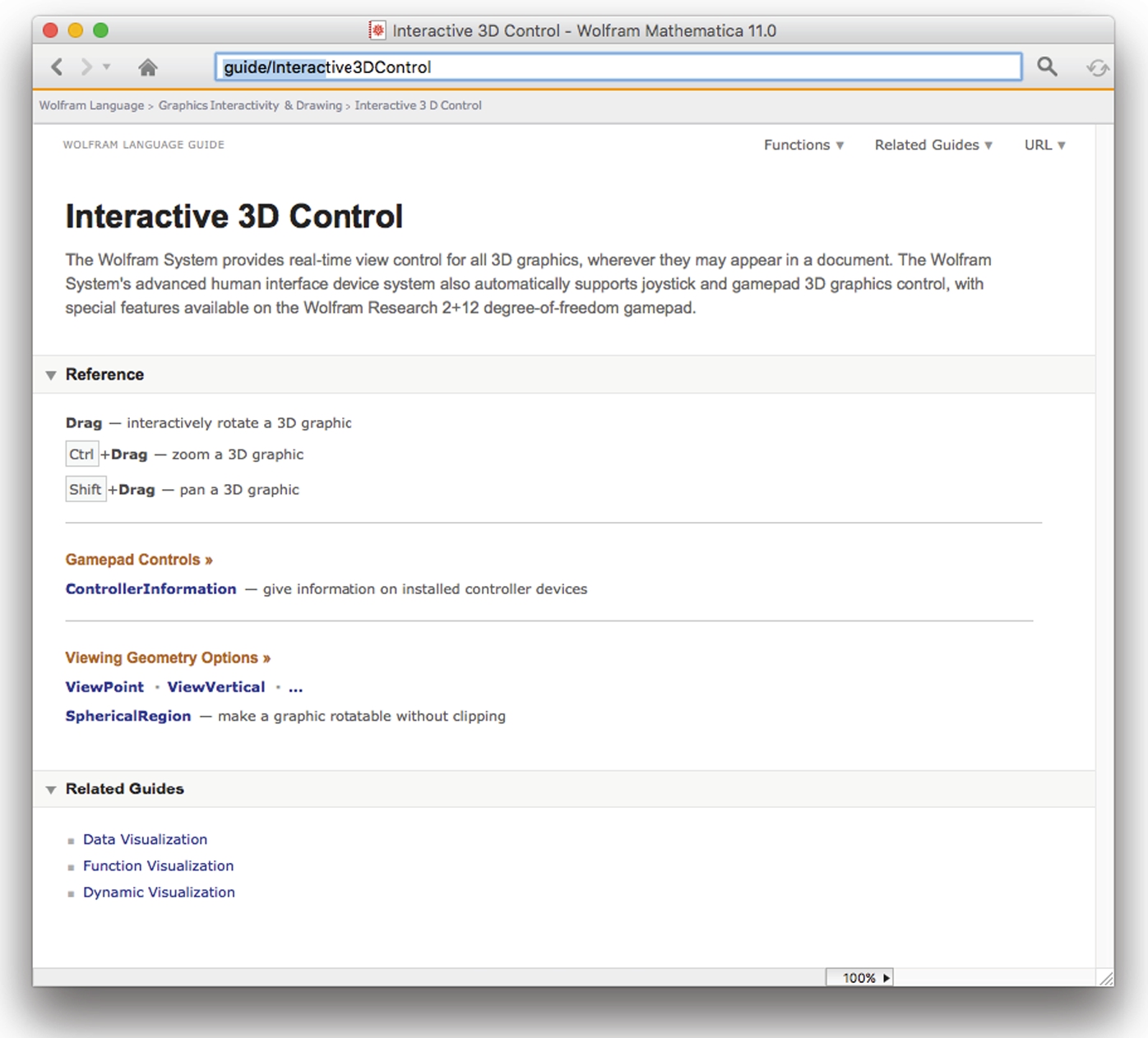
Manually, use the ViewPoint option.
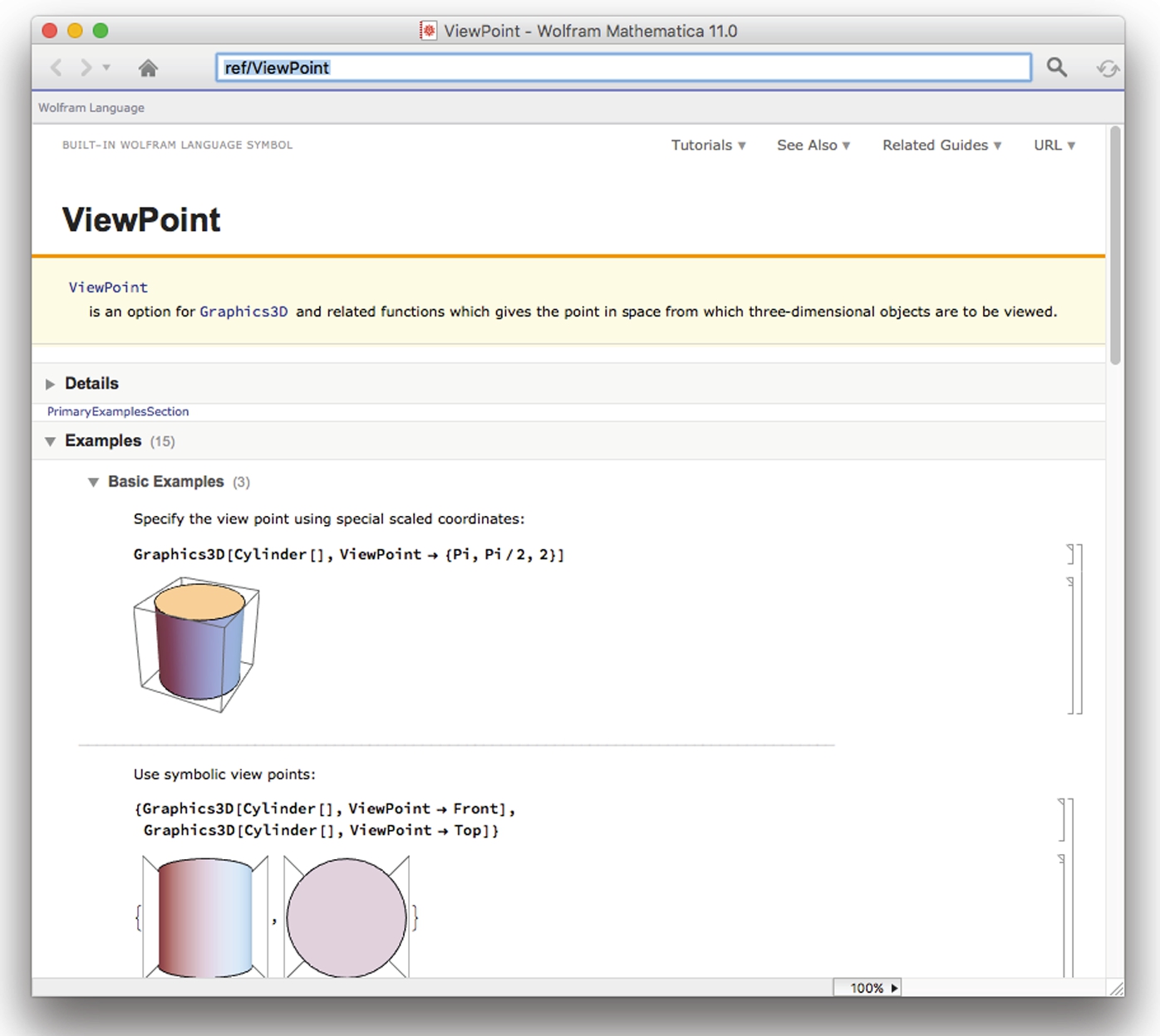
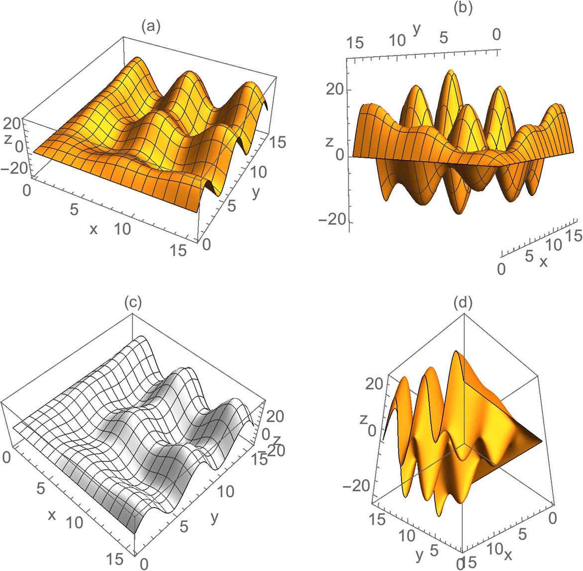
Fig. 2.19 shows four different views of the graph of ![]() for
for ![]() and
and ![]() . The options AxesLabel, BoxRatios, ViewPoint, PlotPoints, Shading, and Mesh are also illustrated.
. The options AxesLabel, BoxRatios, ViewPoint, PlotPoints, Shading, and Mesh are also illustrated.
 for 0 ⩽ x ⩽ 5π.
![]()
![]()
![]()
![]()
![]()
![]()
![]()
![]()
![]()
![]()
![]()
![]()
![]()
![]()
![]()
![]()
![]()
![]()
![]()
![]()
ContourPlot is especially useful when graphing equations. The graph of the equation ![]() , where C is a constant, is the same as the contour plot of
, where C is a constant, is the same as the contour plot of ![]() corresponding to C. That is, the graph of
corresponding to C. That is, the graph of ![]() is the same as the level curve of
is the same as the level curve of ![]() corresponding to
corresponding to ![]() .
.
Use ContourPlot to graph equations of the form ![]() with
with
ContourPlot[f[x,y]==g[x,y],{x,a,b},{y,c,d}].
Example 2.29
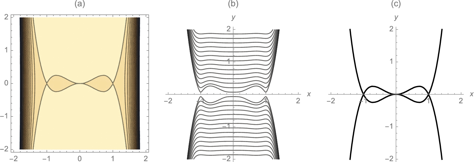
Graph the equation ![]() for
for ![]() .
.
Solution
We define ![]() to be the left-hand side of the equation
to be the left-hand side of the equation ![]() and then use ContourPlot to graph eq for
and then use ContourPlot to graph eq for ![]() in Fig. 2.20.
in Fig. 2.20.
![]()
![]()
![]()
![]()
![]()
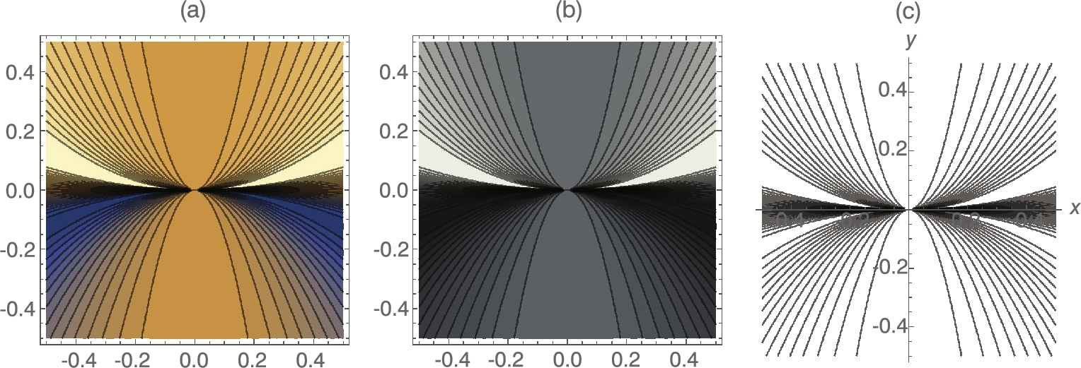
To graph the contour plots of ![]() for particular values of C, create a list of the values of C for which you want the contour plots and then use the option Contours->List of C values.
for particular values of C, create a list of the values of C for which you want the contour plots and then use the option Contours->List of C values.
For example, here we use Table to create a list of 30 equally spaced values of ![]() for
for ![]() .
.
![]()
Next, we use ContourPlot to graph ![]() for each C-value in vals and illustrate various options associated with the ContourPlot function.
for each C-value in vals and illustrate various options associated with the ContourPlot function.
![]()
![]()
![]()
![]()
![]()
![]()
![]()
![]()
Finally, we use Show together with GraphicsRow to display all three graphics side-by-side in Fig. 2.20.
![]() □
□
Equations can be plotted together, as with the commands Plot and Plot3D, with
ContourPlot[{eq1,eq2,...,eqn},{x,a,b},{y,c,d}].
Example 2.30
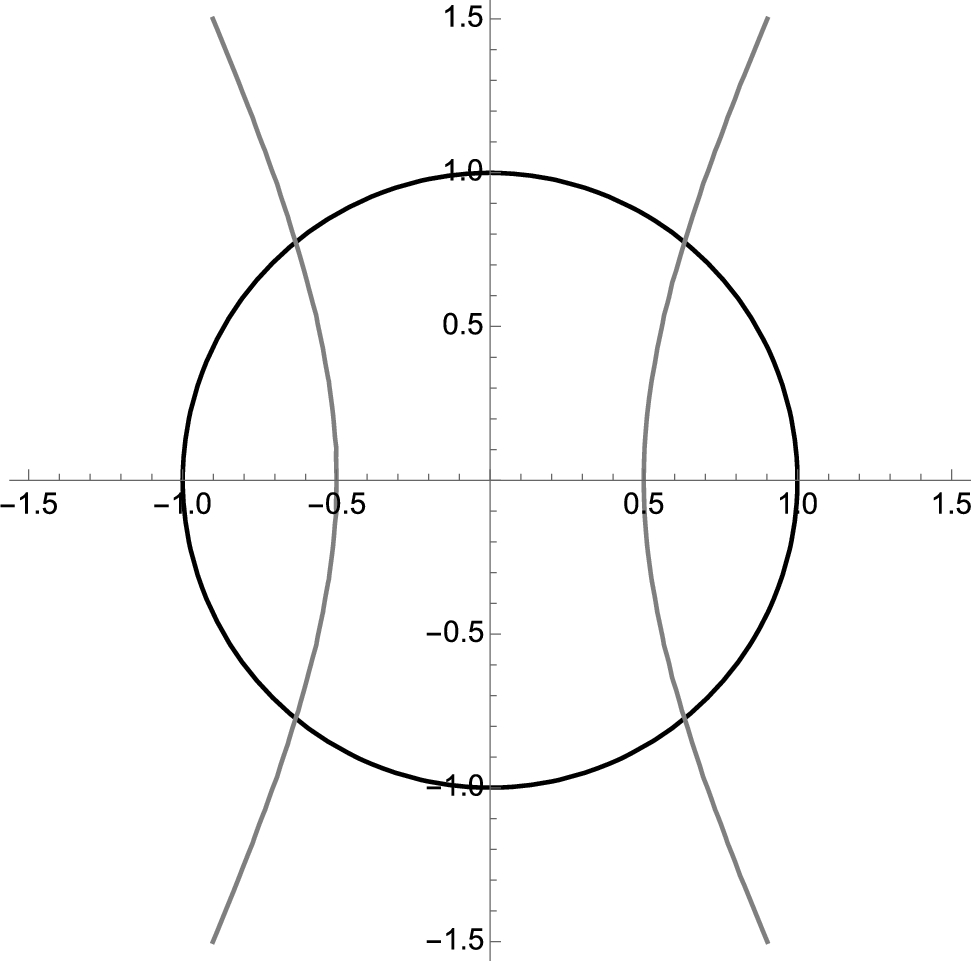
Graph the equations ![]() and
and ![]() for
for ![]() .
.
Solution
We use ContourPlot to graph the equations together on the same axes in Fig. 2.21. The graph of ![]() is the unit circle while the graph of
is the unit circle while the graph of ![]() is a hyperbola.
is a hyperbola.
![]()
![]()
![]()
![]()
From Fig. 2.21, we see four intersection points. To solve an equation of the form ![]() for x, use Solve. Solve[f[x]==g[x],x] attempts to solve the equation
for x, use Solve. Solve[f[x]==g[x],x] attempts to solve the equation ![]() for x. For a system of two equations in two variables, try using Solve[{f[x,y]==0,g[x,y]==0},{x,y}] to solve the system
for x. For a system of two equations in two variables, try using Solve[{f[x,y]==0,g[x,y]==0},{x,y}] to solve the system ![]() ,
, ![]() . Solve will be discussed in more detail in the next section.
. Solve will be discussed in more detail in the next section.
![]()
![]() □
□
Example 2.31
Conic Sections
A conic section is a graph of the equation
Except when the conic is degenerate, the conic ![]() is a (an)
is a (an)
1. Ellipse or circle if ![]() ;
;
2. Parabola if ![]() ; or
; or
3. Hyperbola if ![]() .
.
Graph the conic section ![]() for
for ![]() and for a, b, and c equal to all possible combinations of −1, 1, and 2.
and for a, b, and c equal to all possible combinations of −1, 1, and 2.
Solution
We begin by defining conic to be the equation ![]() and then use Permutations to produce all possible orderings of the list of numbers
and then use Permutations to produce all possible orderings of the list of numbers ![]() , naming the resulting output vals.
, naming the resulting output vals.
![]()
![]()
![]()
![]()
Next we define the function p. Given a1, b1, and c1, p defines toplot to be the equation obtained by replacing a, b, and c in conic by a1, b1, and c1, respectively. Then, toplot is graphed for ![]() . The function p returns a graphics object.
. The function p returns a graphics object.
![]()
![]()
![]()
![]()
![]()
]
We then use Map to compute p for each ordered triple in vals. The resulting output, named graphs, is a set of six graphics objects.
![]()
Partition is then used to partition graphs into three element subsets. The resulting array of graphics objects named toshow is displayed with Show and GraphicsGrid in Fig. 2.22.
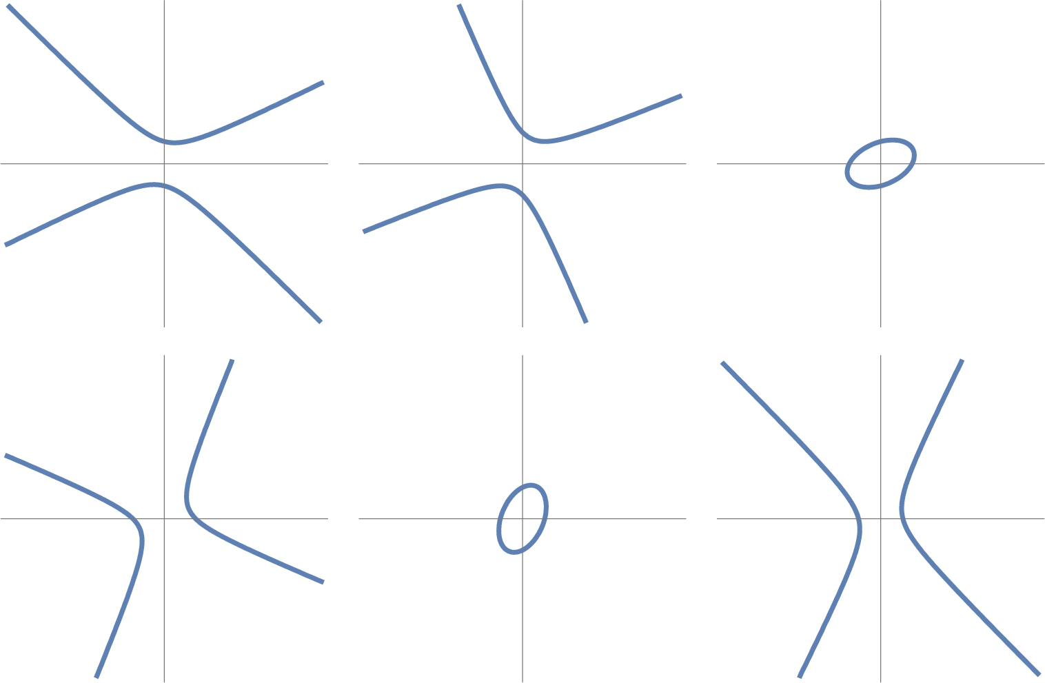
![]() □
□
Studying how parameter values affect the conic is particularly well-suited to a Manipulate object as illustrated in the following commands and then in Fig. 2.23.
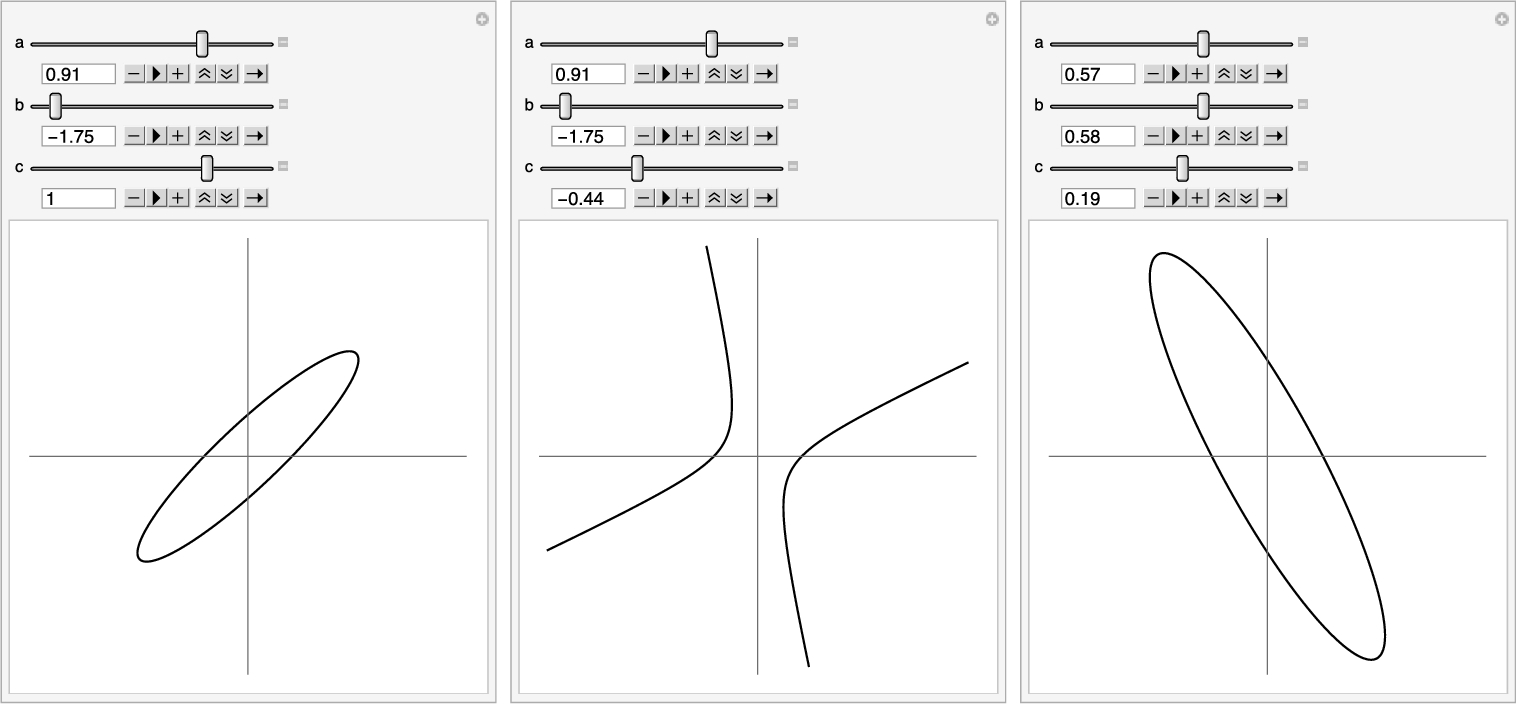
![]()
![]()
![]()
![]()
![]()
2.3.4 Parametric Curves and Surfaces in Space
The command
ParametricPlot3D[{x[t],y[t],z[t]},{t,a,b}]
generates the three-dimensional curve 
![]() and the command
and the command
ParametricPlot3D[{x[u,v],y[u,v],z[u,v]},{u,a,b},{v,c,d}]
plots the surface 
![]() ,
, ![]() .
.
Entering Information[ParametricPlot3D] or ??ParametricPlot3D returns a description of the ParametricPlot3D command along with a list of options and their current settings.
Example 2.32
Umbilic Torus NC
A parametrization of umbilic torus NC is given by ![]() ,
, ![]() ,
, ![]() , where
, where
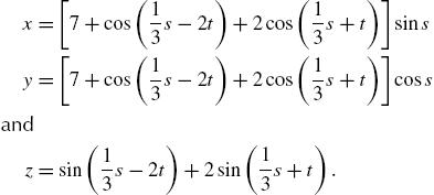
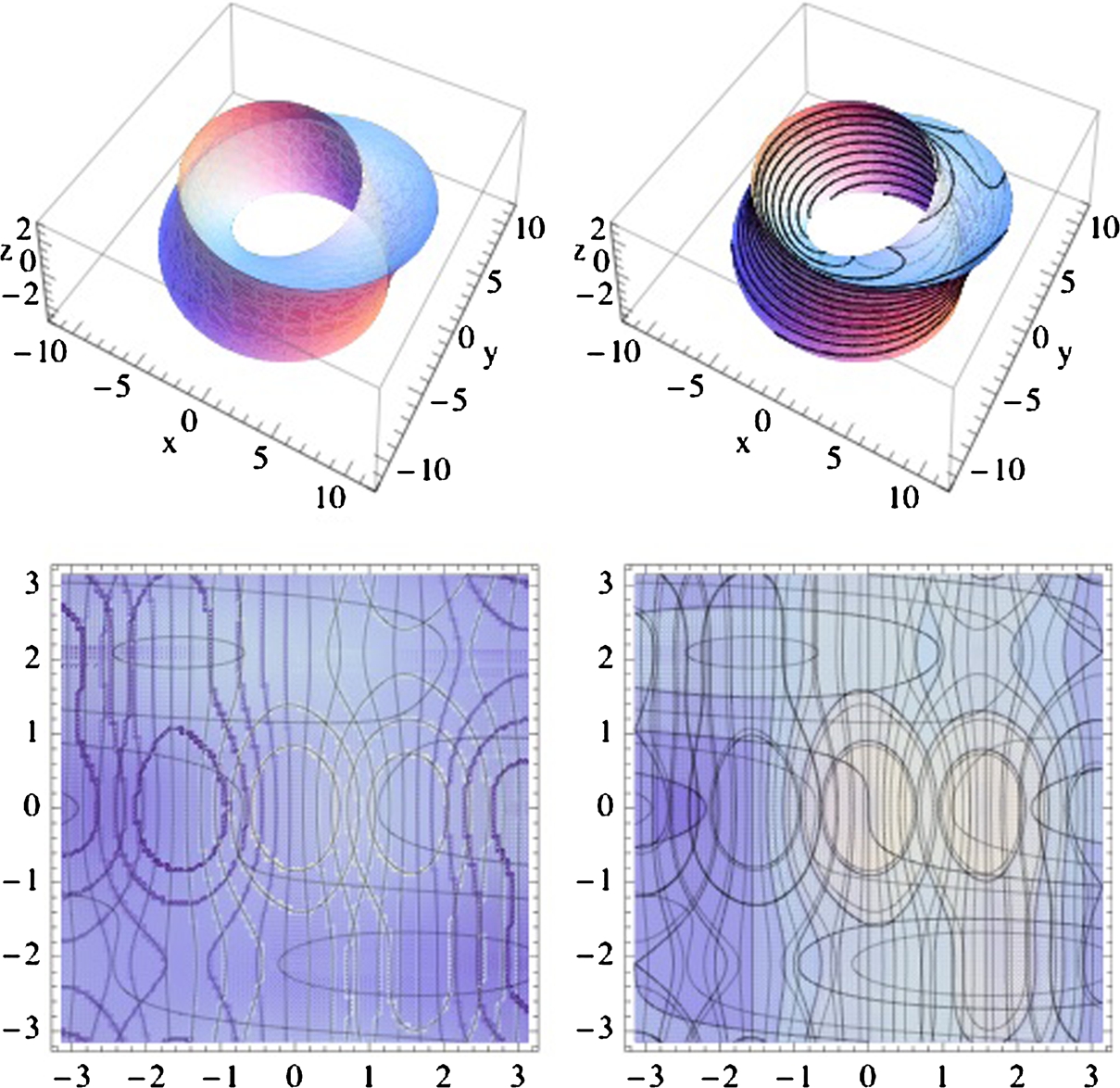
Graph the torus.
Solution
We define ![]() ,
, ![]() ,
, ![]() , and
, and ![]() .
.
![]()
![]()
![]()
![]()
![]()
![]()
The torus is then graphed with ParametricPlot3D, DensityPlot, and ContourPlot in Fig. 2.24. In the plots, we illustrate the Mesh, MeshFunctions, PlotPoints, and PlotRange options. All four plots are shown together with Show and GraphicsGrid. Notice that DensityPlot and ContourPlot yield very similar results: a basic density plot is similar to a basic contour plot but without the contour lines.
![]()
![]()
![]()
![]()
![]()
![]()
![]()
![]()
![]()
![]()
![]()
![]()
![]()
![]()
![]()
![]()
![]()
![]()
![]()
![]()
![]()
![]()
![]()
![]() □
□
Example 2.33
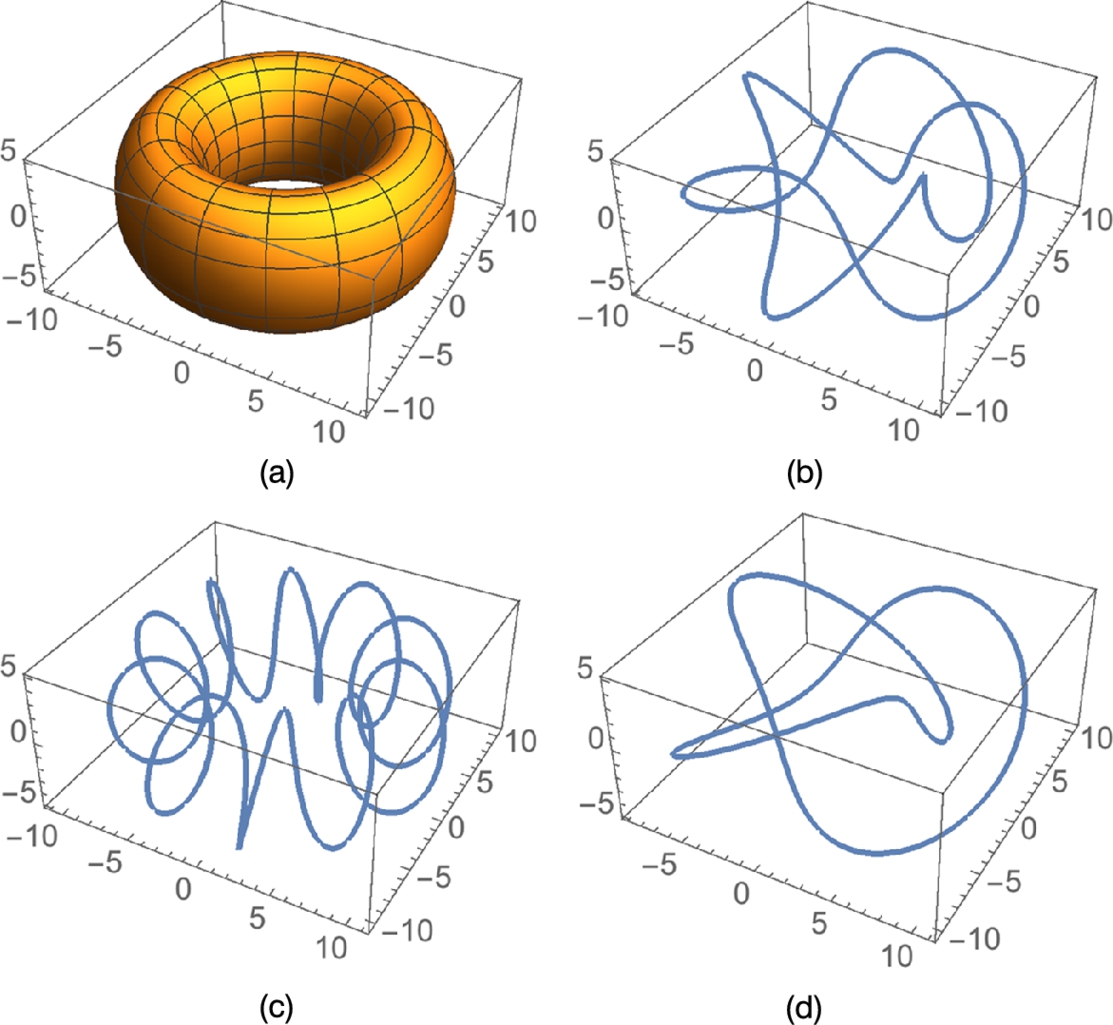
Gray's Torus Example
A parametrization of an elliptical torus is given by
For positive integers p and q, the curve with parametrization
winds around the elliptical torus and is called a torus knot.
Plot the torus if ![]() ,
, ![]() , and
, and ![]() and then graph the torus knots for
and then graph the torus knots for ![]() and
and ![]() ,
, ![]() and
and ![]() , and
, and ![]() and
and ![]() .
.
Solution
We begin by defining torus and torusknot.
![]()
![]()
![]()
![]()
Next, we use ParametricPlot3D to generate all four graphs
![]()
![]()
![]()
![]()
![]()
![]()
![]()
![]()
and show the result as a graphics array with Show and GraphicsGrid in Fig. 2.25.
![]()
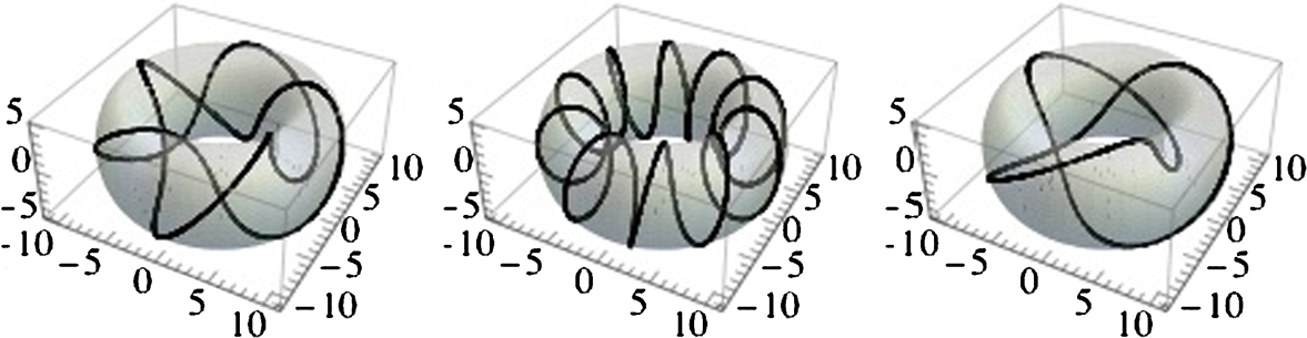
If we take advantage of a few options, such as eliminating the mesh (Mesh->False) and increasing the opacity (PlotStyle->Opacity[.4]), we can produce a graphic of the knot on the torus. After using the PlotStyle option together with Opacity, we produce a nearly transparent torus. Then, each knot is plotted. To assure smooth plots, we increase the number of points plotted with PlotPoints and also increase the thickness of the curve with Thickness.
![]()
![]()
![]()
![]()
![]()
![]()
![]()
![]()
![]()
![]()
We use Show twice together with GraphicsRow to first display the torus with each knot and then display all three graphics side-by-side in Fig. 2.26.
![]() □
□
Example 2.34
Quadric Surfaces
The quadric surfaces are the three-dimensional objects corresponding to the conic sections in two dimensions. A quadric surface is a graph of
where A, B, C, D, E, F, G, H, I, and J are constants.
The intersection of a plane and a quadric surface is a conic section.
Several of the basic quadric surfaces, in standard form, and a parametrization of the surface are listed in the following table.
| Name | Parametric Equations |
| Ellipsoid | |
|
|
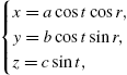 −π/2 ⩽ t ⩽ π/2, −π ⩽ r ⩽ π −π/2 ⩽ t ⩽ π/2, −π ⩽ r ⩽ π |
| Hyperboloid of One Sheet | |
|
|
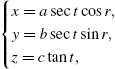 −π/2 < t < π/2, −π ⩽ r ⩽ π −π/2 < t < π/2, −π ⩽ r ⩽ π |
| Hyperboloid of Two Sheets | |
|
|
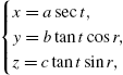 −π/2 < t < π/2 or π/2 < t < 3π/2, −π ⩽ r ⩽ π −π/2 < t < π/2 or π/2 < t < 3π/2, −π ⩽ r ⩽ π |
Graph the ellipsoid with equation ![]() , the hyperboloid of one sheet with equation
, the hyperboloid of one sheet with equation ![]() , and the hyperboloid of two sheets with equation
, and the hyperboloid of two sheets with equation ![]() .
.
Solution
A parametrization of the ellipsoid with equation ![]() is given by
is given by
which is graphed with ParametricPlot3D.
![]()
![]()
![]()
![]()
![]()
![]()
A parametrization of the hyperboloid of one sheet with equation ![]() is given by
is given by
Because ![]() and
and ![]() are undefined if
are undefined if ![]() , we use ParametricPlot3D to graph these parametric equations on a subinterval of
, we use ParametricPlot3D to graph these parametric equations on a subinterval of ![]() ,
, ![]() .
.
![]()
![]()
![]()
![]()
![]()
![]()
pp1 and pp2 are shown together in Fig. 2.27 using Show and GraphicsRow.

 . (b) Plot of
  .
.
![]()
For (c), we take advantage of the ContourPlot3D function:
ContourPlot3D[f[x,y,z],{x,a,b},{y,c,d},{z,u,v}]
graphs several level surfaces of ![]() .
.
We use ContourPlot3D to graph the equation ![]() in Fig. 2.28 (a), illustrating the use of the PlotPoints, Axes, AxesLabel, and BoxRatios options. In Fig. 2.28 (b), several level surfaces are drawn that illustrate the use of the Opacity function with the ContourStyle and Mesh options.
in Fig. 2.28 (a), illustrating the use of the PlotPoints, Axes, AxesLabel, and BoxRatios options. In Fig. 2.28 (b), several level surfaces are drawn that illustrate the use of the Opacity function with the ContourStyle and Mesh options.
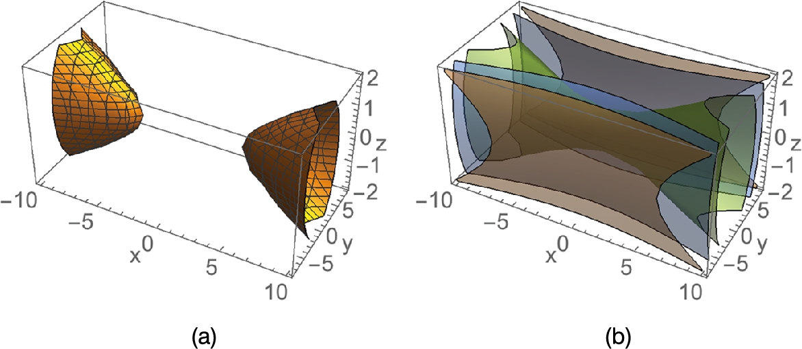
 generated with ContourPlot3D. (b) Several level surfaces of
  .
.
![]()
![]()
![]()
![]()
![]()
![]()
![]()
![]()
![]()
![]()
![]() □
□
ContourPlot3D is especially useful in plotting equations involving three variables x, y, and z for which it is difficult to solve for one variable as a function of the other two.
Example 2.35
Cross-Cap
The Cross-Cap has equation
We use ContourPlot3D to generate the plot of the Cross-Cap shown in Fig. 2.29

![]()
![]()
![]()
![]()
Example 2.36
A homotopy from the Roman surface to the Boy surface is given by
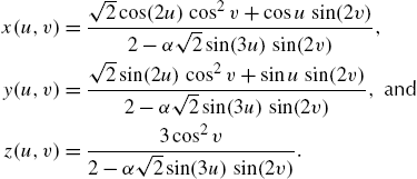
Here, ![]() gives the Roman surface and
gives the Roman surface and ![]() gives the Boy surface.
gives the Boy surface.
If f and g are functions from X to Y, a homotopy from f to g is a continuous function H from ![]() to Y satisfying
to Y satisfying ![]() and
and ![]() .
.
To see the homotopy we first define x, y, z, and ![]() .
.
![]()
![]()
![]()
![]()
![]()
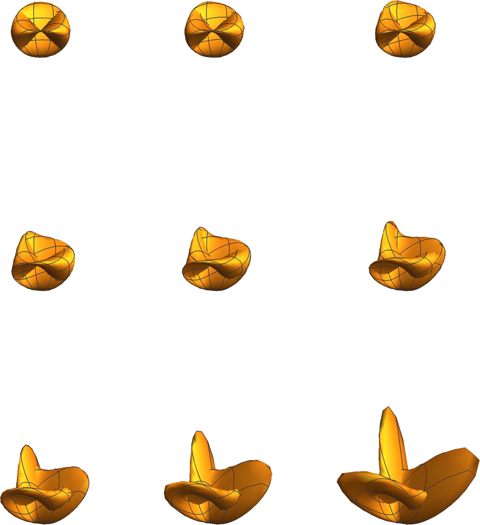
We then use Table together with ParametricPlot3D to parametrically plot x, y, and z, ![]() ,
, ![]() for nine equally spaced values of α between 0 and 1. Note that if the semi-colon is omitted at the end of the command, the nine plots are displayed.
for nine equally spaced values of α between 0 and 1. Note that if the semi-colon is omitted at the end of the command, the nine plots are displayed.
![]()
![]()
![]()
![]()
We then use Partition to partition smalltable into three element subsets. The resulting ![]() array of graphics is shown as a grid with Show together with GraphicsGrid in Fig. 2.30.
array of graphics is shown as a grid with Show together with GraphicsGrid in Fig. 2.30.
![]()
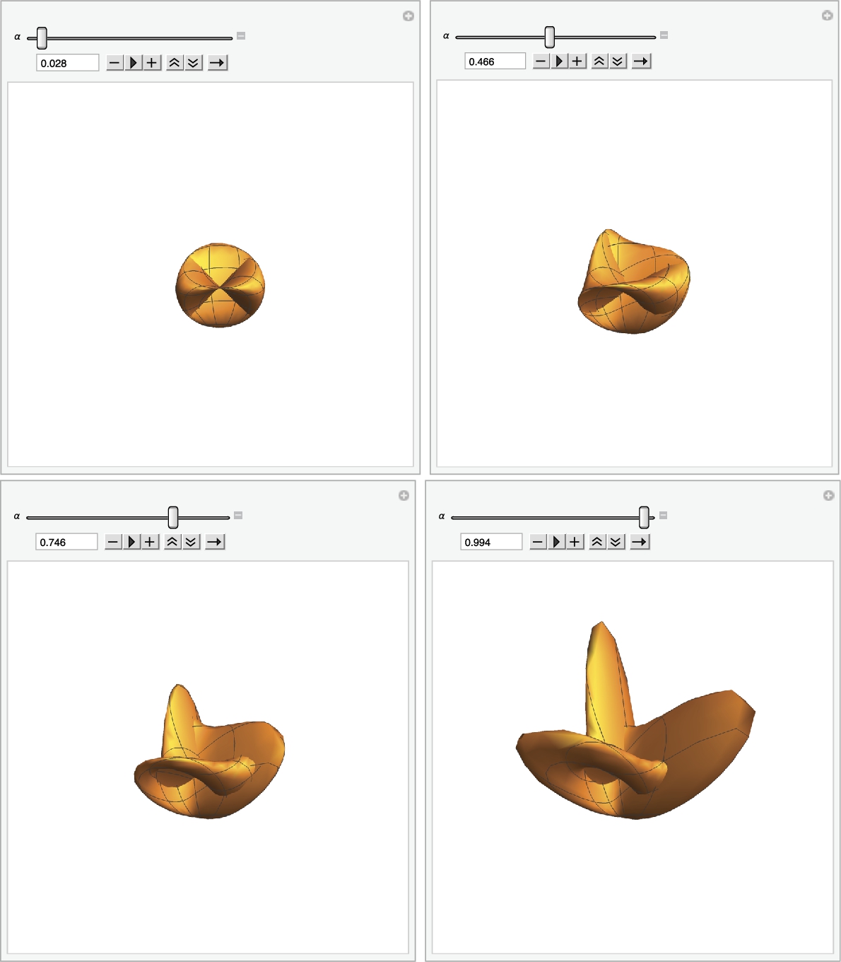
Another way of seeing the transformation is to use Manipulate. Manipulate is very powerful. In its most basic form, Manipulate[f[x],{x,a,b}] creates an interactive display of ![]() for x values from a to b. Because the previous commands depended only on α, we combine the commands into a single Manipulate object that depends on α.
for x values from a to b. Because the previous commands depended only on α, we combine the commands into a single Manipulate object that depends on α.
![]()
![]()
![]()
![]()
![]()
![]()
![]()
![]()
![]()
![]()
![]()
![]()
Several images from the result are shown in Fig. 2.31.
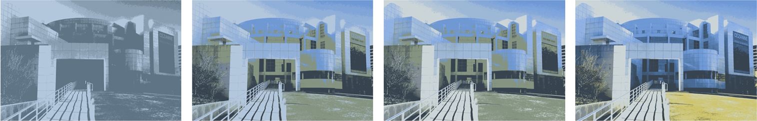
Manipulation of graphics is discussed in more detail in Section 5.6, Matrices and Graphics. Here, we simply illustrate a few quick ways to manipulate a basic jpeg that illustrate a few of the features of Mathematica 11.
Mathematica 11 provides numerous ways to adjust digital images.
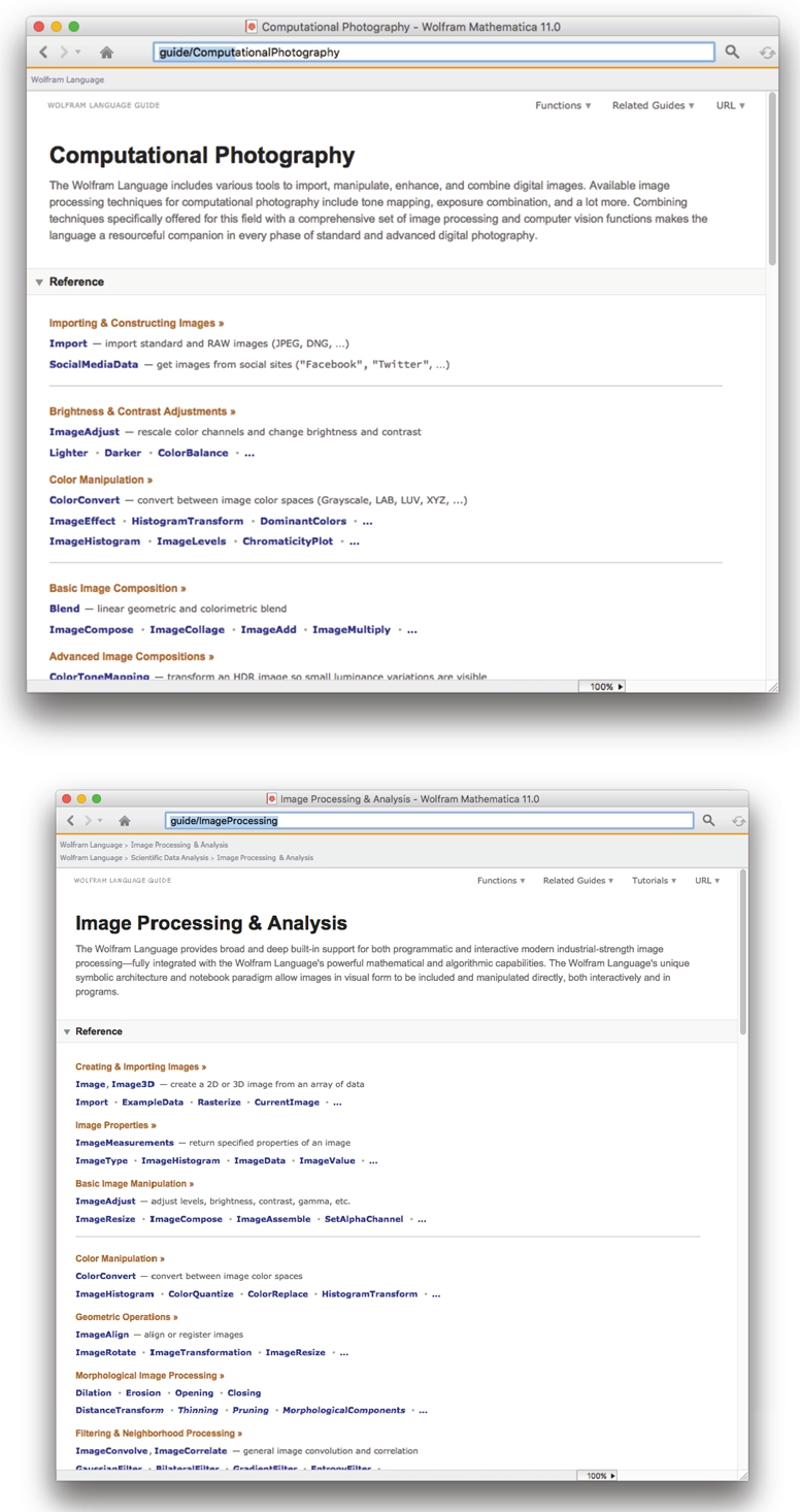
Generally, be sure the graphics file that you want to adjust is in the same folder/directory as the open Mathematica notebook. Use Import["file"] to import the file into your open Mathematica notebook. Keep in mind that these graphics can be assigned names just like any other Mathematica objects. Thus, use assign, =, to assign a name to each graphic as you make adjustments. Finally, use Export, Export["file.ext",expr] to export your modified graphic expr using the name file.ext, where ext is usually something similar to jpg or pdf. You can then move those graphics into your favorite photography or printing program so you can fine-tune the adjustments and then print the results.
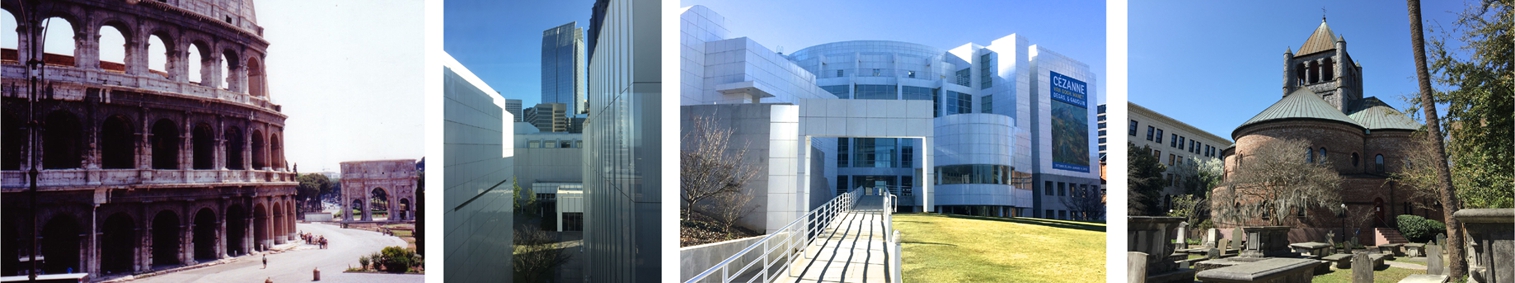
Example 2.37
We use Import to import a few graphics into Mathematica. The four graphs are displayed in a row using Show and GraphicsRow in Fig. 2.32.
![]()
![]()
![]()
![]()
![]()
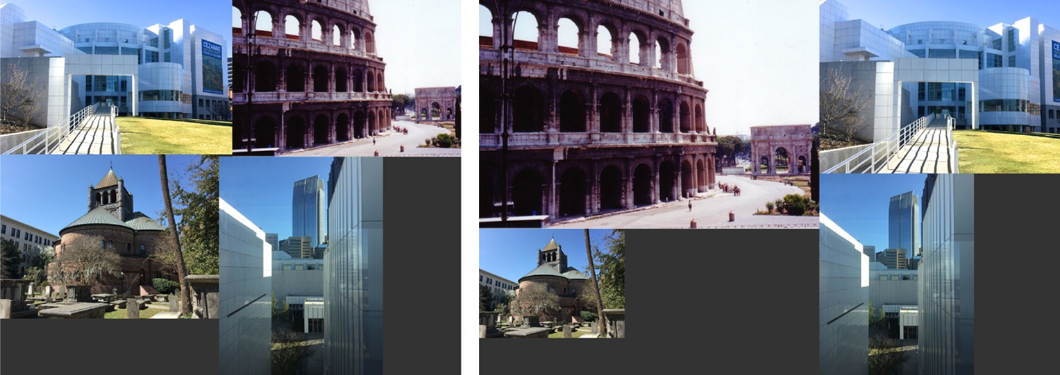
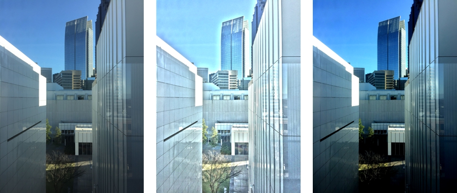
Mathematica's tools for editing digital images are quite extensive. Here, we illustrate just a few of the basic available functions. You can combine graphics together with ImageCollage. The command
ImageCollage[{n1->image1,n2->image2,...,nm->imagem}]
creates a collage that weights the various images according to the n-value (see Fig. 2.33).
![]()
![]()
![]()
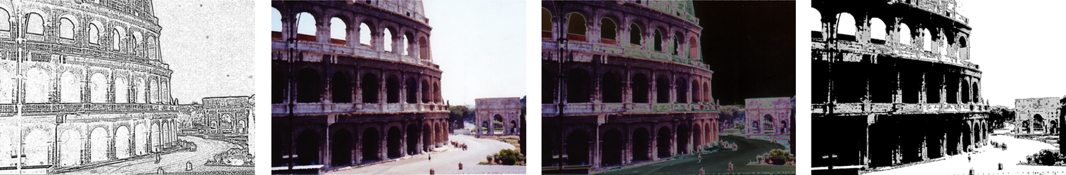
ImageEffect can be used to apply various effects to an image. Use ?ImageEffect for a comprehensive discussion of the different effects that are available (see Fig. 2.34).
![]()
![]()
![]()
![]()
![]()
DominantColors returns a list of the dominant colors in a graphic (see Fig. 2.35).
![]()
![]()
You can then use commands like ColorQuantize to approximate an image with n discrete colors. Later, we will use ImageApply to change the colors of individual pixels.
![]()
![]()
![]()
![]()
![]()
ColorToneMapping transforms an image so that you can see small variations in color. On the other hand, ImageAdjust adjusts the color levels (see Fig. 2.36).
![]()
![]()
![]()
2.3.5 Miscellaneous Comments
Clearly, Mathematica's graphics capabilities are extensive and volumes could be written about them. You can see many commands that we haven't discussed here by using ? to see those commands that contain the string Plot.
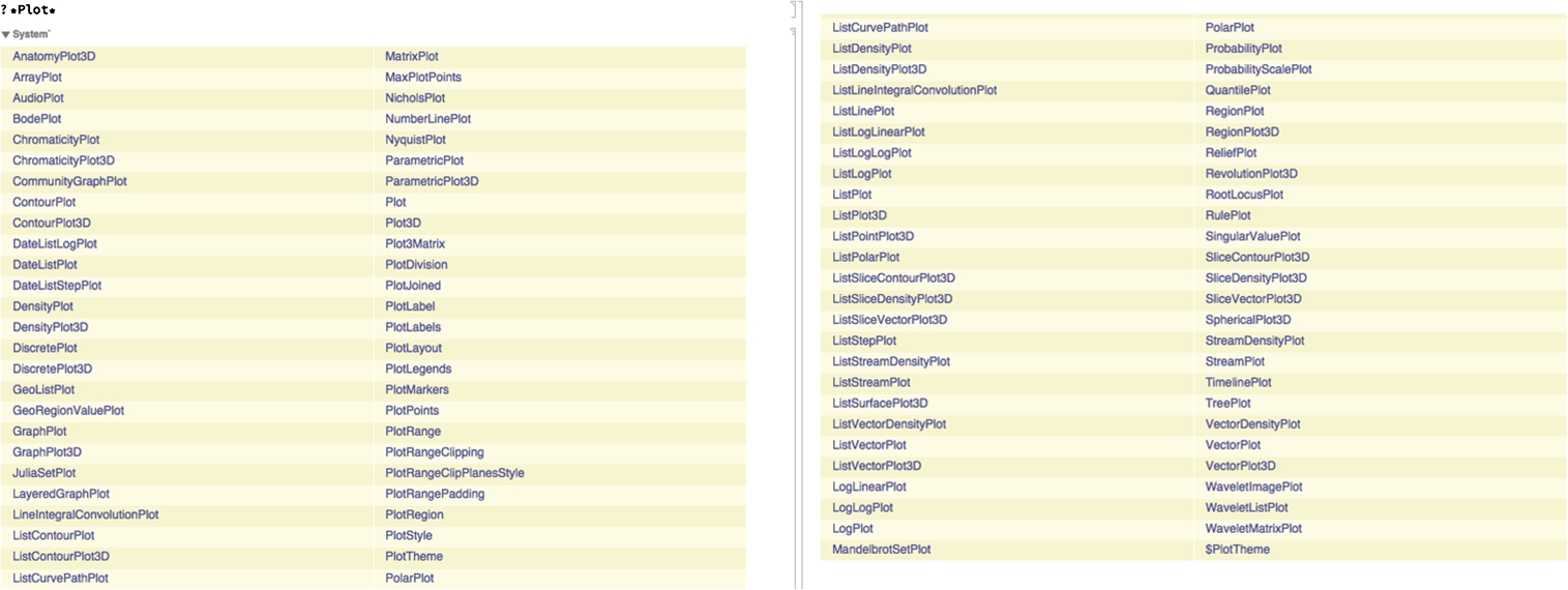
You can obtain detailed information regarding any of these commands from the Documentation Center by clicking on the command's name.
For now, we briefly mention a few of the ones that were not discussed previously. To plot lists of numbers or lists of ordered pairs, use ListPlot or ListLinePlot, which are discussed in more detail in Chapter 4. For matrices and other arrays use commands such as MatrixPlot or ArrayPlot that are discussed in more detail in Chapter 4.
Example 2.38
Cellular Automaton
Very loosly speaking, a cellular automaton is a discrete function that assigns values to subsequent rows based on the values of the cells in the previous row(s). For a concise discussion of cellular automaton refer to Weisstein (Weisstein, Eric W. “Cellular Automaton.” From MathWorld–A Wolfram Web Resource. http://mathworld.wolfram.com/CellularAutomaton.html), CellularAutomatan is a powerful command that allows you to investigate (quite complicated) cellular automaton. In its simplest form,
CellularAutomaton[rule,initialvalues,n]
returns the first n generations of the cellular automaton following the specified rule and having the indicated initial values.
The simplest cellular automaton are called elementary cellular automaton (Weisstein, Eric W. “Elementary Cellular Automaton.” From MathWorld–A Wolfram Web Resource. http://mathworld.wolfram.com/ElementaryCellularAutomaton.html). Based on basic counting principals, there are 256 elementary cellular automaton. They are cataloged by number. With
![]()
![]()
![]()
![]()
![]()
we calculate the first five generations of the elementary cellular automaton with a 1 at position 0 on generation 0 using Rule 146. To calculate the first 100 generations, we use CellularAutomaton[146, {{1},0}, 100]. The resulting array is rather large so we use ArrayPlot to visualize it in Fig. 2.37 (a). Using our color scheme, the cells with value 1 are shaded in red and those with 0 are in light green.
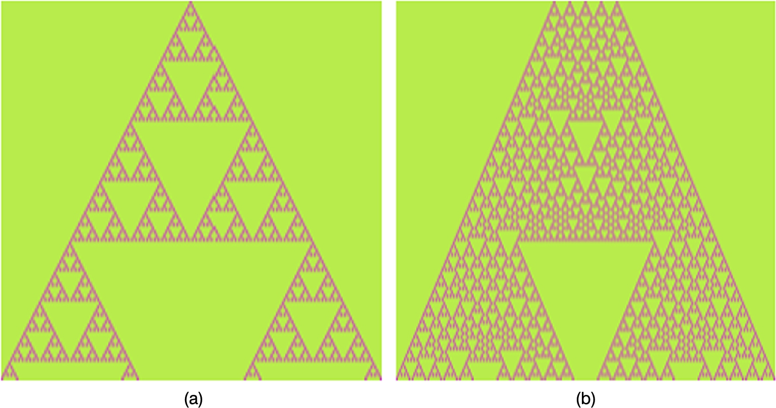
![]()
![]()
In this case the grid is initially spaced so that positions 1, 11, 21, 31, and 41 have the value one. The first three generations using Rule 146 are calculated.
![]()
![]()
![]()
![]()
![]()
![]()
![]()
![]()
![]()
![]()
To see how the situation evolves over 100 generations is more easily seen using ArrayPlot. See Fig. 2.37 (b)
![]()
![]()
![]()
![]()
Of the 256 elementary cellular automaton, many are equivalent. To see that some of them are equivalent, we create a plot of the 256 elementary cellular automaton for 50 generations as done with Rule 146. All 256 plots are shown on the left in Fig. 2.38 (a). With Union, we remove and sort the ones that are identically equal. Those are shown on the right in Fig. 2.38 (b).
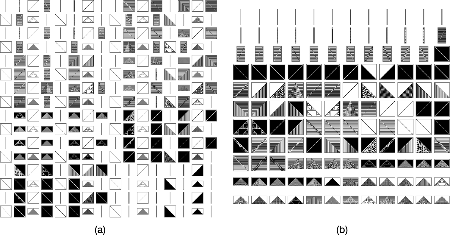
![]()
![]()
![]()
![]()
![]()
![]()
![]()
![]()
To see the plots together with the rule number, use Table. Each ordered pair returned consists of the rule number and the 50 generation plot. To display the ordered pairs in an organized fashion, we use Grid. Of course, the result is quite large so just a portion of the actual grid is displayed in Fig. 2.39.
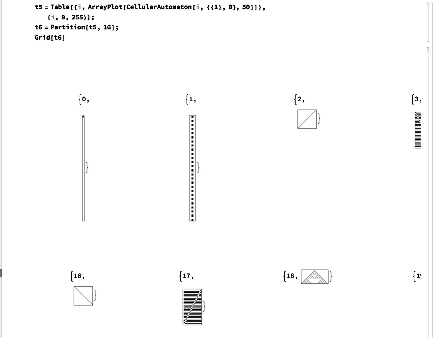
![]()
![]()
![]()
![]()
Note that MatrixPlot and ArrayPlot are discussed in more detail in Chapter 5.
For graphs that involve points or nodes or connecting them by edges (graph theory), you can use GraphPlot to help investigate some problems. For trees, use TreePlot.
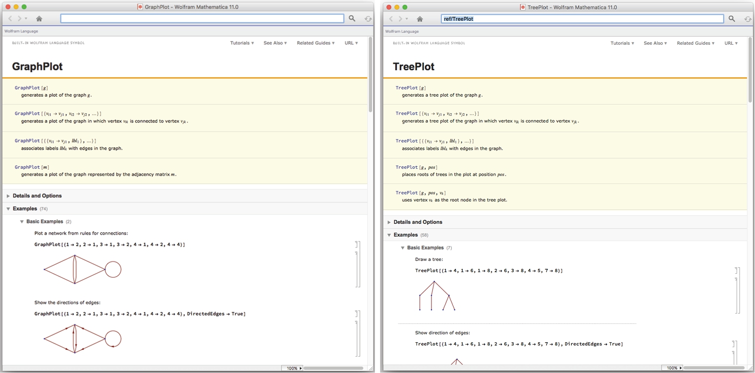
Example 2.39
Graceful graphs don't have multiple edges or loops.
We generate O with GraphPlot and display the result in Fig. 2.40 (a).
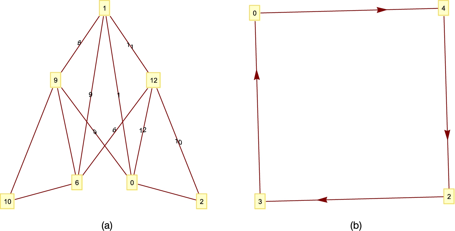
![]()
![]()
![]()
![]()
![]() is shown in Fig. 2.40 (b).
is shown in Fig. 2.40 (b).
![]()
![]()
Replacing GraphPlot with TreePlot gives us Fig. 2.41.
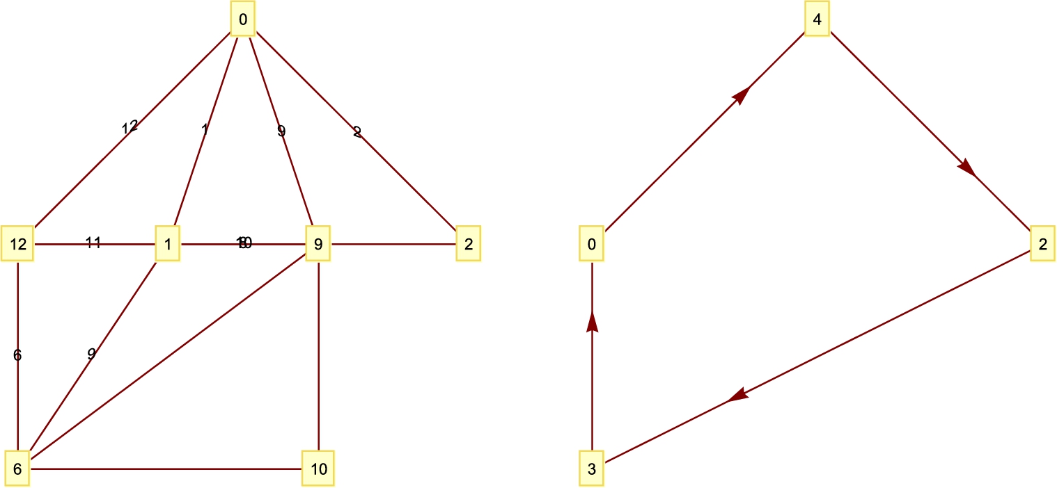
![]()
![]()
![]()
![]()
![]()
![]()
2.4 Solving Equations
2.4.1 Exact Solutions of Equations
Mathematica can find exact solutions to many equations and systems of equations, including exact solutions to polynomial equations of degree four or less. Because a single equals sign “=” is used to name objects and assign values in Mathematica, equations in Mathematica are of the form
left-hand side==right-hand side.
The “double-equals” sign “==” between the left-hand side and right-hand side specifies that the object is an equation. For example, to represent the equation ![]() in Mathematica, type 3x+7==4. The command Solve[lhs==rhs,x] solves the equation
in Mathematica, type 3x+7==4. The command Solve[lhs==rhs,x] solves the equation ![]() for x. If the only unknown in the equation
for x. If the only unknown in the equation ![]() is x and Mathematica does not need to use inverse functions to solve for x, the command Solve[lhs==rhs] solves the equation
is x and Mathematica does not need to use inverse functions to solve for x, the command Solve[lhs==rhs] solves the equation ![]() for x. Hence, to solve the equation
for x. Hence, to solve the equation ![]() , both the commands Solve[3x+7==4] and Solve[3x+7==4,x] return the same result.
, both the commands Solve[3x+7==4] and Solve[3x+7==4,x] return the same result.
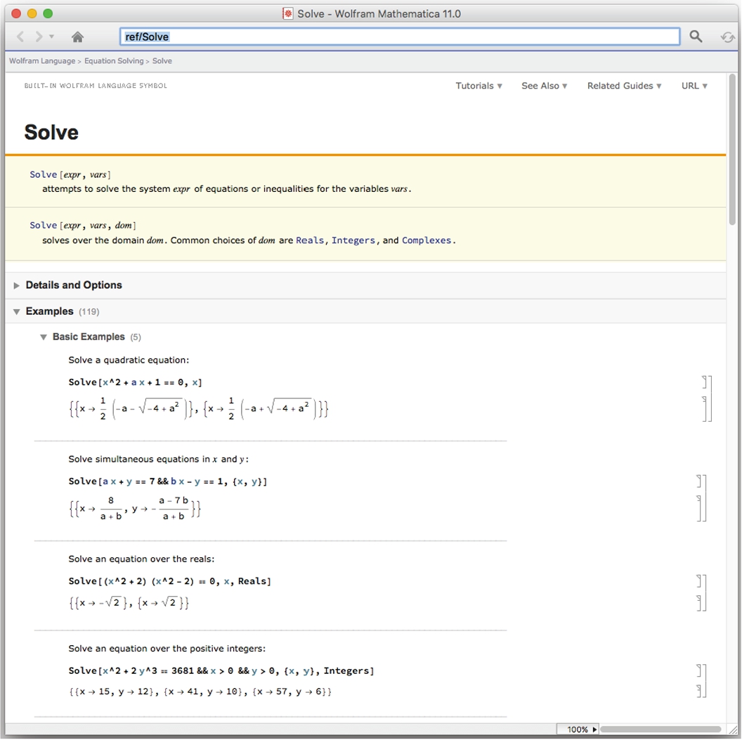
Example 2.40
Solve the equations ![]() ,
, ![]() , and
, and ![]() .
.
Solution
In each case, we use Solve to solve the indicated equation. Be sure to include the double equals sign “==” between the left and right-hand sides of each equation. Thus, the result of entering
![]()
![]()
means that the solution of ![]() is
is ![]() and the result of entering
and the result of entering
![]()
![]()
means that the solution of ![]() is
is ![]() . On the other hand, the equation
. On the other hand, the equation ![]() has two imaginary roots. We see that entering
has two imaginary roots. We see that entering
![]()
![]()
yields all three solutions. Thus, the solutions of ![]() are
are ![]() and
and ![]() . Remember that the Mathematica symbol I represents the complex number
. Remember that the Mathematica symbol I represents the complex number ![]() . In general, Mathematica can find the exact solutions of any polynomial equation of degree four or less. □
. In general, Mathematica can find the exact solutions of any polynomial equation of degree four or less. □
Observe that the results of a Solve command are a list.
Mathematica can also solve equations involving more than one variable for one variable (literal equations) in terms of other unknowns.
Example 2.41
(a) Solve the equation ![]() for h. (b) Solve the equation
for h. (b) Solve the equation ![]() for a.
for a.
Solution
These equations involve more than one unknown so we must specify the variable for which we are solving in the Solve commands. Thus, entering
![]()
![]()
solves the equation ![]() for h. (Be sure to include a space or * between π and r.) Similarly, entering
for h. (Be sure to include a space or * between π and r.) Similarly, entering
![]()
![]()
solves the equation ![]() for a. □
for a. □
If Mathematica needs to use inverse functions to solve an equation, you must be sure to specify the variable(s) for which you want Mathematica to solve.
Example 2.42
Find a solution of ![]() .
.
Solution
When the command Solve[Sin[x]^2-2Sin[x]-3==0] is entered, Mathematica solves the equation for Sin[x]. However, when the command
Solve[Sin[x]^2-2Sin[x]-3==0,x]
is entered, Mathematica attempts to solve the equation for x.
![]()
![]()
![]()
![]()
![]()
Mathematica's result indicates that the solutions to the equation are ![]() and
and ![]() , where C is any integer.
, where C is any integer. ![]() is not a real number so in the context of solving the equation, we ignore the complex-valued solutions. Therefore this equation has infinitely many solutions of the form
is not a real number so in the context of solving the equation, we ignore the complex-valued solutions. Therefore this equation has infinitely many solutions of the form ![]() ,
, ![]() , ±1, ±2, ...;
, ±1, ±2, ...; ![]() has no solutions. □
has no solutions. □
Example 2.43
Let ![]() ,
, ![]() . (a) Solve
. (a) Solve ![]() . (b) Graph
. (b) Graph ![]() and
and ![]() .
.
Solution
After defining ![]() , we use D to compute
, we use D to compute ![]() and then use Solve to solve
and then use Solve to solve ![]() .
.
D[f[x],x] computes ![]() ; D[f[x],{x,n}] computes
; D[f[x],{x,n}] computes ![]() . Topics from calculus are discussed in more detail in Chapter 3.
. Topics from calculus are discussed in more detail in Chapter 3.
![]()
![]()
![]()
![]()
![]()
![]()
![]()
As in the previous example, the solutions are given as a sequence of conditionals: ![]() ,
, ![]() and
and ![]() , where C is an integer. Of these infinitely many solutions,
, where C is an integer. Of these infinitely many solutions, ![]() ,
, ![]() , and
, and ![]() are in the interval
are in the interval ![]() .
.
To verify by hand, we use the identity ![]() and factor:
and factor:
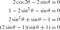
so ![]() or
or ![]() . Because we are assuming that
. Because we are assuming that ![]() , we obtain the solutions
, we obtain the solutions ![]() ,
, ![]() , or
, or ![]() . We perform the same steps with Mathematica.
. We perform the same steps with Mathematica.
expression /. x->y replaces all occurrences of x in ![]() by y.
by y.
![]()
![]()
![]()
![]()
![]()
![]()
Finally, we graph ![]() and
and ![]() with Plot in Fig. 2.42. Note that the plot is drawn to scale because we include the option AspectRatio->Automatic.
with Plot in Fig. 2.42. Note that the plot is drawn to scale because we include the option AspectRatio->Automatic.
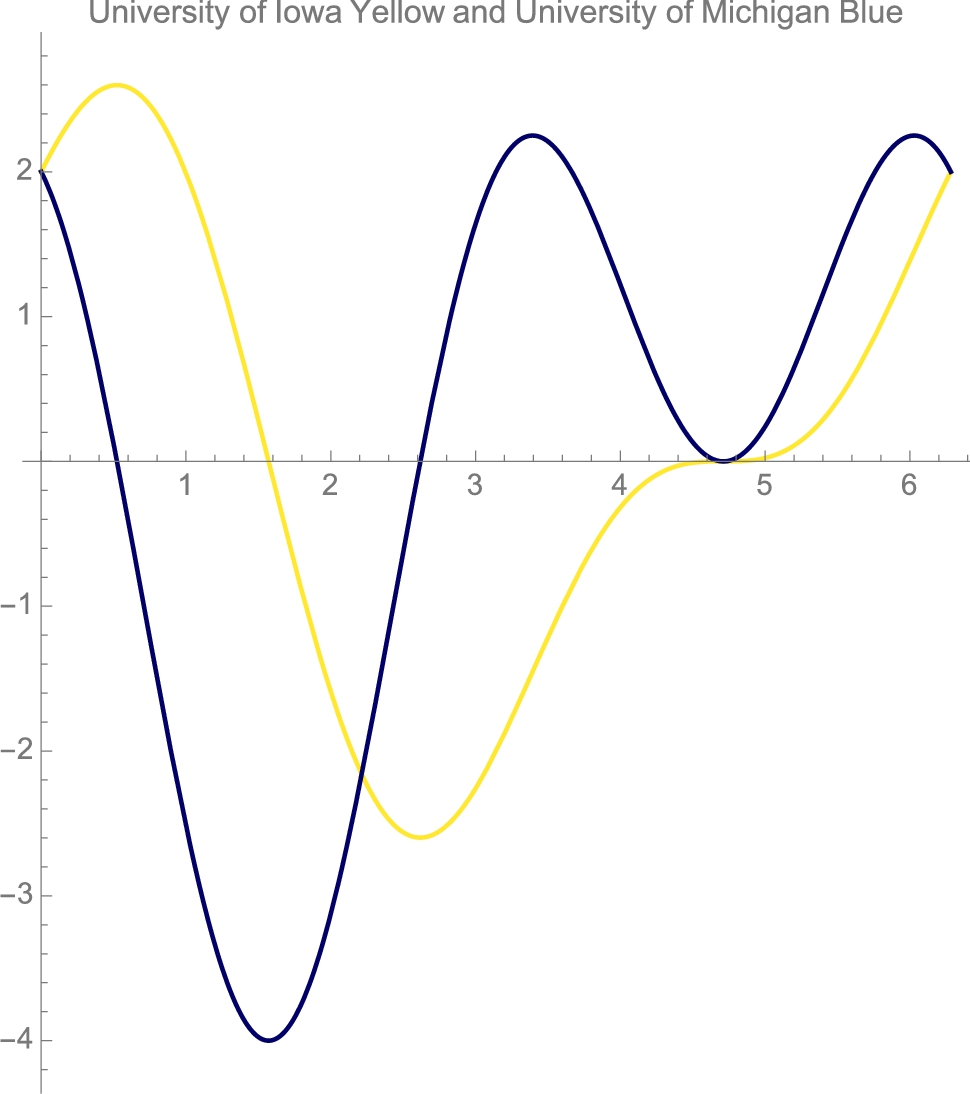
![]()
![]()
![]() □
□
We can also use Solve to find the solutions, if any, of various types of systems of equations. Entering
Solve[{lhs1==rhs1,lhs2==rhs2},{x,y}]
solves a system of two equations for x and y while entering
Solve[{lhs1==rhs1,lhs2==rhs2}]
attempts to solve the system of equations for all unknowns. In general, Solve can find the solutions to a system of linear equations. In fact, if the systems to be solved are inconsistent or dependent, Mathematica's output indicates so.
Example 2.44
Solve each system: (a) ![]() ; (b)
; (b) 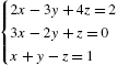 ; (c)
; (c) 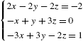 ; and (d)
 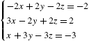 .
.
Solution
In each case we use Solve to solve the given system. For (a), the result of entering
![]()
![]()
means that the solution of ![]() is
is ![]() , which is the point of intersection of the lines with equations
, which is the point of intersection of the lines with equations ![]() and
and ![]() . See Fig. 2.43 (a).
. See Fig. 2.43 (a).
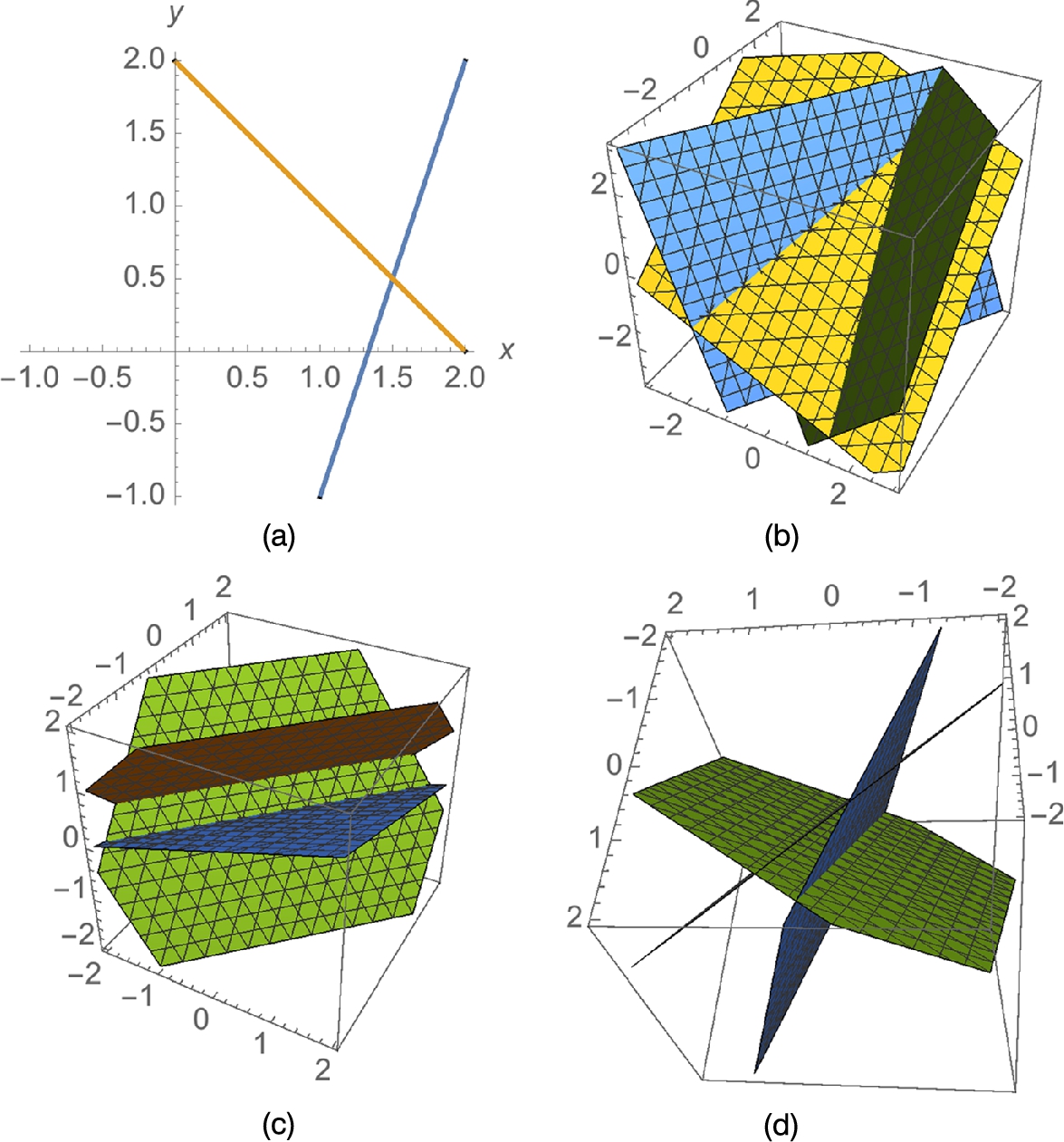
![]()
![]()
![]()
![]()
(b) We can verify that the results returned by Mathematica are correct. First, we name the system of equations sys and then use Solve to solve the system of equations naming the result sols.
![]()
![]()
![]()
![]()
We verify the result by substituting the values obtained with Solve back into sys with ReplaceAll (/.).
![]()
![]()
means that the solution of 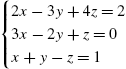 is
is ![]() , which is the point of intersection of the planes with equations
, which is the point of intersection of the planes with equations ![]() ,
, ![]() ,
, ![]() . See Fig. 2.43 (b).
. See Fig. 2.43 (b).
![]()
![]()
![]()
To better see the intersection point, click within the graphic and then drag to an appropriate viewing angle.
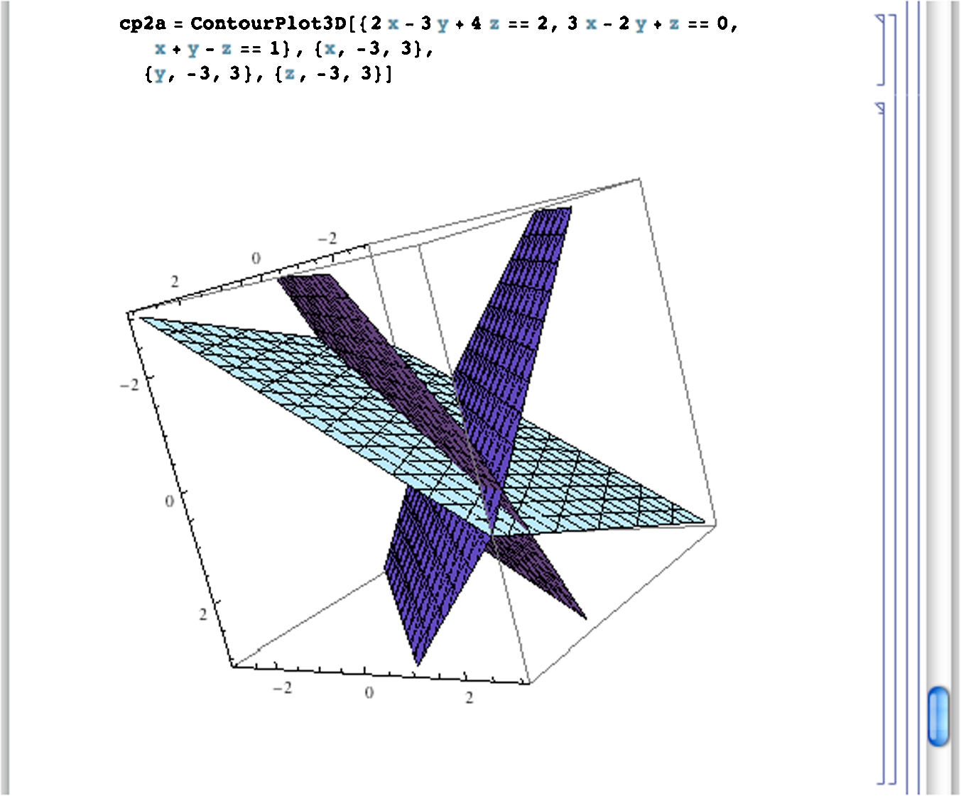
(c) When we use Solve to solve this system, Mathematica returns {}, which indicates that the system has no solution; the system is inconsistent.
![]()
{}
To see that the planes with equations ![]() ,
, ![]() , and
, and ![]() have no points in common, graph them with in Fig. 2.43 (c).
have no points in common, graph them with in Fig. 2.43 (c).
![]()
![]()
![]()
To better see that the planes do not intersect, we click and drag the graphic to an appropriate viewing angle.
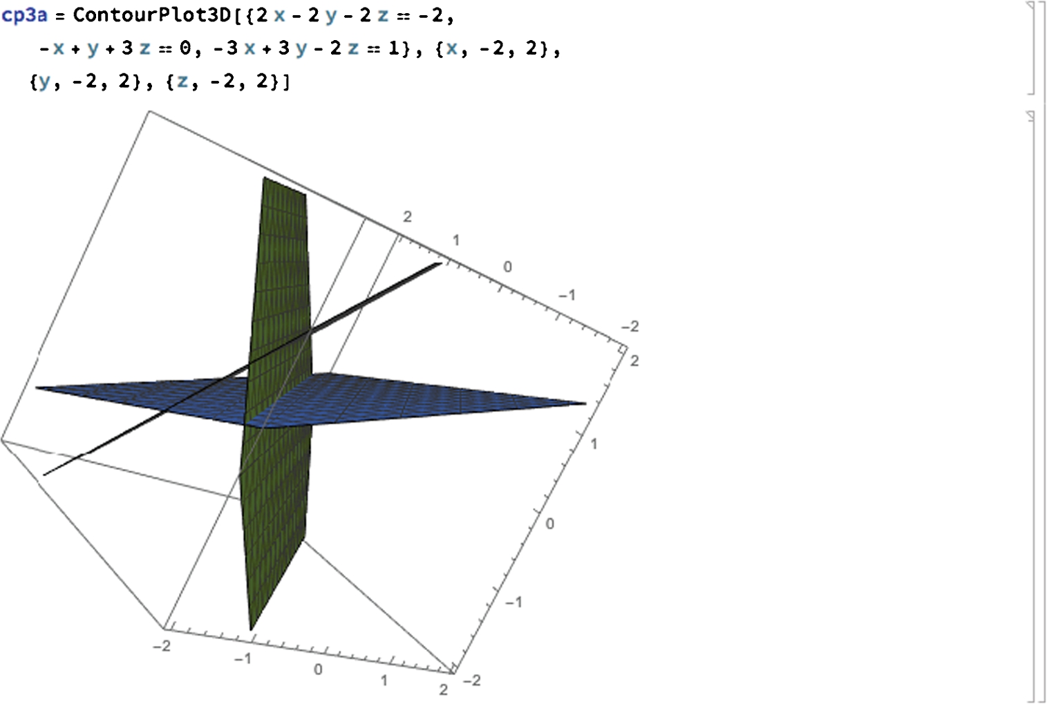
(d) On the other hand, when we use Solve to solve this system, Mathematica's result indicates that the system has infinitely many solutions. That is, all ordered triples of the form ![]() are solutions of the system.
are solutions of the system.
![]()
![]()
![]()
We see that the intersection of the three planes is a line with ContourPlot3D. See Fig. 2.43 (d).
![]()
![]()
![]()
![]() □
□
We can often use Solve to find solutions of a nonlinear system of equations as well.
Example 2.45
Solve the systems (a) ![]() and (b)
and (b) ![]() (a, b greater than zero) for x and y.
(a, b greater than zero) for x and y.
Solution
The graphs of the equations are both ellipses. We use ContourPlot to graph each equation, naming the results cp1 and cp2, respectively, and then use Show to display both graphs together in Fig. 2.44 (a). The solutions of the system correspond to the intersection points of the two graphs. Alternatively, the solutions of the system correspond to the intersection points of the level curves of ![]() and
and ![]() corresponding to 0. See Fig. 2.44 (b).
corresponding to 0. See Fig. 2.44 (b).
![]()
![]()
![]()
![]()
![]()
![]()
![]()
![]()
![]()
![]()
Finally, we use Solve to find the solutions of the system.
.1in
![]()
![]()
For (b), we also use Solve to find the solutions of the system. However, because the unknowns in the equations are a, b, m, x, and y, we must specify that we want to solve for x and y in the Solve command.
![]()
![]() □
□
Although Mathematica can find the exact solution to every polynomial equation of degree four or less, exact solutions to some equations may not be meaningful. In those cases, Mathematica can provide approximations of the exact solutions using either the N[expression] or the expression // N commands.
Example 2.46
Approximate the solutions to the equations (a) ![]() ; and (b)
; and (b) ![]() .
.
Solution
Each of these is a polynomial equation with degree less than five so Solve will find the exact solutions of each equation. However, the solutions are quite complicated so we use N to obtain approximate solutions of each equation. For (a), entering
![]()
![]()
![]()
first finds the exact solutions of the equation ![]() and then computes approximations of those solutions. The resulting output is the list of approximate solutions. Approximating solutions of equations is discussed further in the next subsection.
and then computes approximations of those solutions. The resulting output is the list of approximate solutions. Approximating solutions of equations is discussed further in the next subsection.
For (b), entering
![]()
![]()
![]()
![]()
![]()
first finds the exact solutions of the equation ![]() and then computes approximations of those solutions. The resulting output is the list of approximate solutions. □
and then computes approximations of those solutions. The resulting output is the list of approximate solutions. □
2.4.2 Approximate Solutions of Equations
When solving an equation is either impractical or impossible, Mathematica provides several functions including FindRoot, NRoots, and NSolve to approximate solutions of equations. NRoots and numerically approximate the roots of any polynomial equation. The command NRoots[poly1==poly2,x] approximates the solutions of the polynomial equation poly1==poly2, where both poly1 and poly2 are polynomials in x. The syntax for NSolve is the same as the syntax of NRoots although NSolve is usually capable of approximating solutions of more complicated equations than NRoots. Often you will find that using Solve together with N will yield the exact same results as those obtained using NSolve. Regardless, it is relatively easy to ask Mathematica to approximate the solutions of a complicated equation and it cannot. In a general sense, solving and approximating solutions of equations in a general sense is a challenging problem.
FindRoot attempts to approximate a root to an equation provided that a “reasonable” guess of the root is given. FindRoot works on functions other than polynomials. The command
FindRoot[lhs==rhs,{x,firstguess}]
searches for a numerical solution to the equation lhs==rhs, starting with x = firstguess. To locate more than one root, FindRoot must be used several times. One way of obtaining firstguess (for real-valued solutions) is to graph both lhs and rhs with Plot, find the point(s) of intersection, and estimate the x-coordinates of the point(s) of intersection. Generally, NRoots is easier to use than FindRoot when trying to approximate the roots of a polynomial. For “simple” non-polynomial equations, NSolve may work well. If NRoots or NSolve do not yield the desired results, it may be best to use FindRoot to approximate each root (solution) individually.
Example 2.47
Approximate the solutions of ![]() .
.
Solution
Because ![]() is a polynomial equation, we may use NRoots to approximate the solutions of the equation. Thus, entering
is a polynomial equation, we may use NRoots to approximate the solutions of the equation. Thus, entering
![]()
![]()
![]()
![]()
![]()
approximates the solutions of ![]() . The symbol || appearing in the result represents “or”.
. The symbol || appearing in the result represents “or”.
We obtain equivalent results with NSolve.
![]()
![]()
![]()
![]()
![]()
FindRoot may also be used to approximate each root of the equation. However, to use FindRoot, we must supply an initial approximation of the solution that we wish to approximate. The real solutions of ![]() correspond to the values of x where the graph of
correspond to the values of x where the graph of ![]() intersects the x-axis. We use Plot to graph
intersects the x-axis. We use Plot to graph ![]() in Fig. 2.45.
in Fig. 2.45.
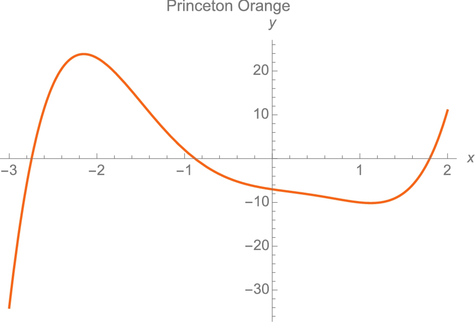
![]()
![]()
![]()
![]()
We see that the graph intersects the x-axis near ![]() , −1, and 1.5. We use these values as initial approximations of each solution. Thus, entering
, −1, and 1.5. We use these values as initial approximations of each solution. Thus, entering
![]()
![]()
approximates the solution near −2.5, entering
![]()
![]()
approximates the solution near −1, and entering
![]()
![]()
approximates the solution near 1.5, which is relatively close to ![]() , which is why we used
, which is why we used ![]() as our initial guess in the FindRoot command. Note that FindRoot may be used to approximate complex solutions as well. To obtain initial guesses, observe that the solutions of
as our initial guess in the FindRoot command. Note that FindRoot may be used to approximate complex solutions as well. To obtain initial guesses, observe that the solutions of ![]() ,
, ![]() , x, y real, are the level curves of
, x, y real, are the level curves of ![]() that are points. In Fig. 2.46, we use ContourPlot to graph various level curves of
that are points. In Fig. 2.46, we use ContourPlot to graph various level curves of ![]() ,
, ![]() ,
, ![]() . In the plot, observe that the two complex solutions occur at
. In the plot, observe that the two complex solutions occur at ![]() .
.
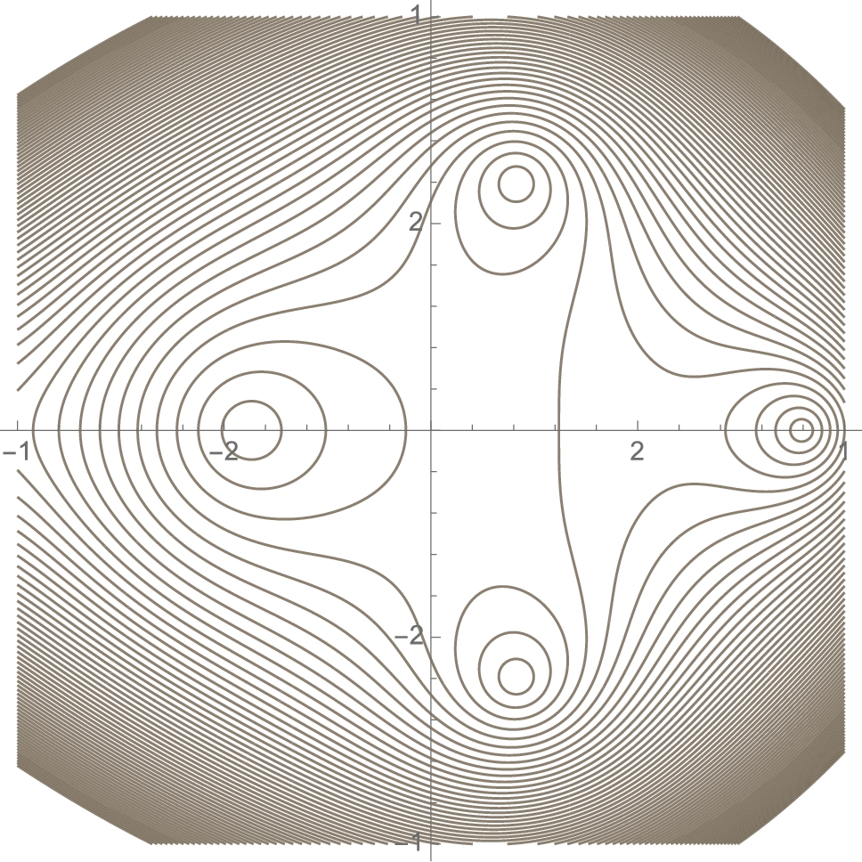
![]()
![]()
![]()
![]()
![]()
Thus, entering
![]()
![]()
approximates the solution near ![]() . For polynomials with real coefficients, complex solutions occur in conjugate pairs so the other complex solution is approximately
. For polynomials with real coefficients, complex solutions occur in conjugate pairs so the other complex solution is approximately ![]() .
.
Example 2.48
Find the first three nonnegative solutions of ![]() .
.
Solution
We attempt to solve ![]() with Solve.
with Solve.

We next graph ![]() and
and ![]() together in Fig. 2.47.
together in Fig. 2.47.
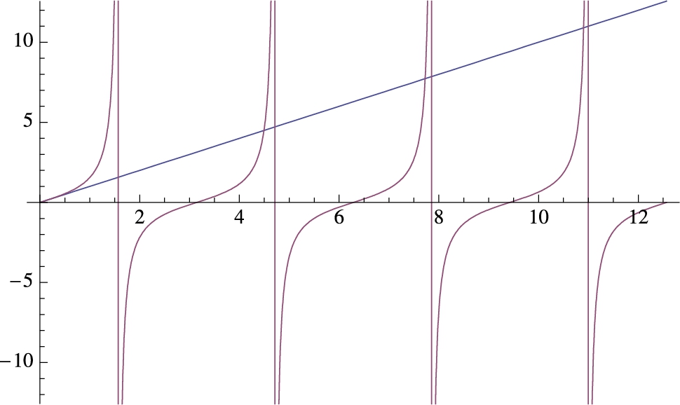 .
.
![]()
![]() □
□
In the graph, we see that ![]() is a solution. This is confirmed with FindRoot.
is a solution. This is confirmed with FindRoot.
Remember that vertical lines are never the graphs of functions. In this case, they represent the vertical asymptotes at odd multiples of ![]() .
.
![]()
![]()
The second solution is near 4 while the third solution is near 7. Using FindRoot together with these initial approximations locates the second two solutions.
![]()
![]()
![]()
![]()
FindRoot can also be used to approximate solutions to systems of equations. (Although NRoots can solve a polynomial equation, NRoots cannot be used to solve a system of polynomial equations.) When approximations of solutions of systems of equations are desired, use either Solve and N together, when possible, or FindRoot.
Example 2.49
Approximate the solutions to the system of equations ![]() .
.
Solution
We begin by using ContourPlot to graph each equation in Fig. 2.48. From the resulting graph, we see that ![]() is a hyperbola,
is a hyperbola, ![]() is an ellipse, and there are four solutions to the system of equations.
is an ellipse, and there are four solutions to the system of equations.
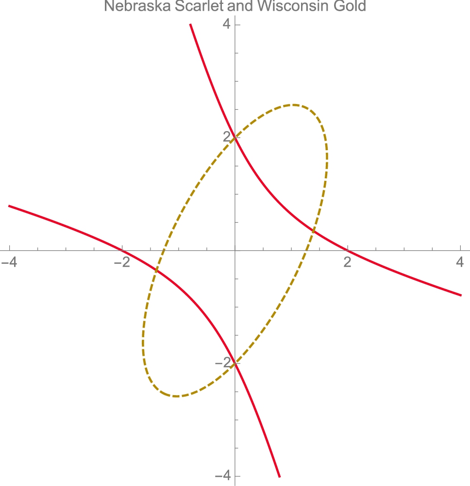
![]()
![]()
![]()
![]()
![]()
![]()
![]()
![]()
![]()
![]()
![]()
From the graph we see that possible solutions are ![]() and
and ![]() . In fact, substituting
. In fact, substituting ![]() and
and ![]() and
and ![]() and
and ![]() into each equation verifies that these points are both exact solutions of the equation. The remaining two solutions are approximated with FindRoot.
into each equation verifies that these points are both exact solutions of the equation. The remaining two solutions are approximated with FindRoot.
![]()
![]()
![]() □
□