Calculus
Abstract
Chapter 3 introduces Mathematica's calculus capabilities. The examples used to illustrate the various functions are similar to examples typically seen in a traditional calculus sequence. If you have trouble typing commands correctly, use the buttons on the Basic Math Input or Basic Math Assistant palettes to help you create templates in standard mathematical notation that you can evaluate.

Keywords
Limits; Differential calculus; Integral calculus; Series calculus; Multi-variable calculus
3.1 Limits and Continuity
One of the first topics discussed in calculus is that of limits. Mathematica can be used to investigate limits graphically and numerically. In addition, the Mathematica command Limit[f[x],x->a] attempts to compute the limit of ![]() as x approaches a,
as x approaches a, ![]() , where a can be a finite number, ∞ (Infinity), or −∞ (-Infinity). The arrow “->” is obtained by typing a minus sign “-” followed by a greater than sign “>”.
, where a can be a finite number, ∞ (Infinity), or −∞ (-Infinity). The arrow “->” is obtained by typing a minus sign “-” followed by a greater than sign “>”.
Remark 3.1
To define a function of a single variable, ![]() , enter f[x_]=expression in x. To generate a basic plot of
, enter f[x_]=expression in x. To generate a basic plot of ![]() for
for ![]() , enter Plot[f[x],{x,a,b}].
, enter Plot[f[x],{x,a,b}].
3.1.1 Using Graphs and Tables to Predict Limits
Example 3.1
Use a graph and table of values to investigate ![]() .
.
Solution
We clear all prior definitions of f, define ![]() , and then graph
, and then graph ![]() on the interval
on the interval ![]() with Plot.
with Plot.
![]()
![]()
![]()
![]()
![]()
From the graph shown in Fig. 3.1, we might, correctly, conclude that ![]() . Further evidence that
. Further evidence that ![]() can be obtained by computing the values of
can be obtained by computing the values of ![]() for values of x “near”
for values of x “near” ![]() . In the following, we use RandomReal. RandomReal[{a,b}] returns a “random” real number between a and b. Because we are generating “random” numbers, your results will differ from those obtained here, to define xvals to be a table of 6 “random” real numbers. The first number in xvals is between −1 and 1, the second between
. In the following, we use RandomReal. RandomReal[{a,b}] returns a “random” real number between a and b. Because we are generating “random” numbers, your results will differ from those obtained here, to define xvals to be a table of 6 “random” real numbers. The first number in xvals is between −1 and 1, the second between ![]() and 1/10, and so on.
and 1/10, and so on.
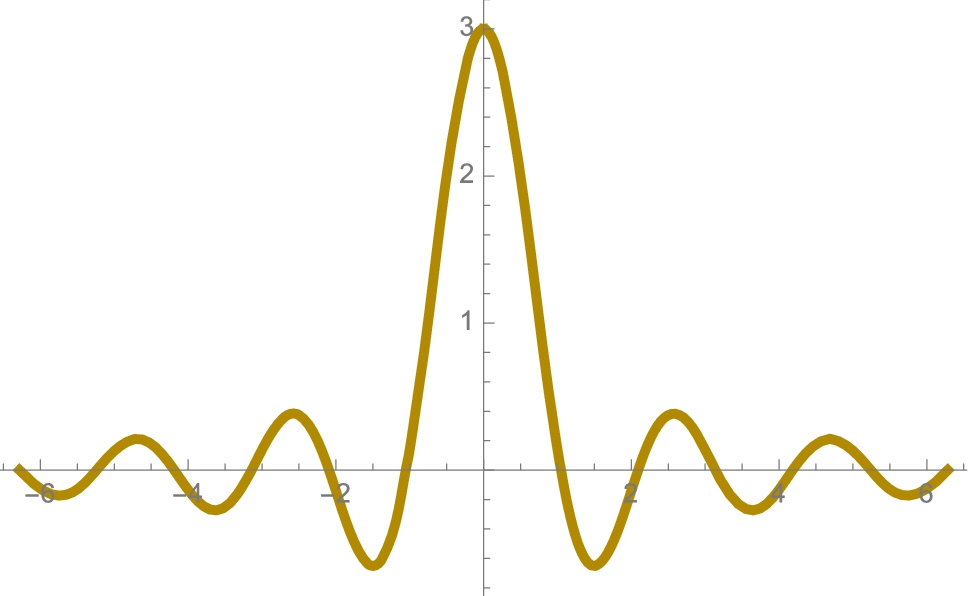
 on the interval [−2π,2π] in Wisconsin gold.
![]()
![]()
![]()
We then use Map to compute the value of ![]() for each x in xvals. Map[f,{x1,x2,...,xn}] returns the list
for each x in xvals. Map[f,{x1,x2,...,xn}] returns the list ![]() . We use Table to display the results in tabular form. Generally, list[[i]] returns the ith element of list while
. We use Table to display the results in tabular form. Generally, list[[i]] returns the ith element of list while
Table[f[i],{i,start,finish,stepsize}]
computes each value of ![]() from start to finish in increments of stepsize. To create a table consisting of n equally spaced values, use stepsize=(finish-start)/(n-1). TableForm attempts to display a table form in a standard format such as the row-and-column format that follows.
from start to finish in increments of stepsize. To create a table consisting of n equally spaced values, use stepsize=(finish-start)/(n-1). TableForm attempts to display a table form in a standard format such as the row-and-column format that follows.
![]()
![]()
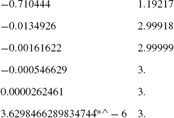
From these values, we might again correctly deduce that ![]() . Of course, these results do not prove that
. Of course, these results do not prove that ![]() but they are helpful in convincing us that
but they are helpful in convincing us that ![]() . □
. □
For piecewise-defined functions, you can either use Mathematica's conditional command (/;) to define the piecewise-defined function or use Piecewise.
Example 3.2
If 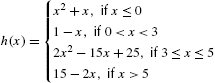 , compute the following limits: (a)
 ![]() , (b)
, (b) ![]() , (c)
, (c) ![]() .
.
Solution
We use Mathematica's conditional command, /; to define h. We must use delayed evaluation (:=) because ![]() cannot be computed unless Mathematica is given a particular value of x. The first line of the following defines
cannot be computed unless Mathematica is given a particular value of x. The first line of the following defines ![]() to be
to be ![]() for
for ![]() , the second line defines
, the second line defines ![]() to be
to be ![]() for
for ![]() and so on. Notice that Mathematica accidentally connects
and so on. Notice that Mathematica accidentally connects ![]() to
to ![]() and then
and then ![]() to
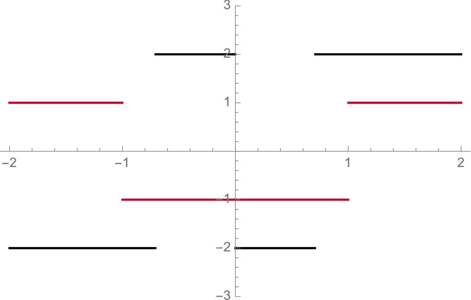
to ![]() . (See Fig. 3.2 (a).) The delayed evaluation is also incompatible with Mathematica's Limit function.
. (See Fig. 3.2 (a).) The delayed evaluation is also incompatible with Mathematica's Limit function.
![]()
![]()
![]()
![]()
![]()
![]()
![]()
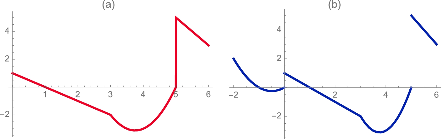
To avoid these problems and see the discontinuities in our plots, we redefine h using Mathematica's Piecewise function as follows.
![]()
![]()
![]()
![]()
![]()
![]()
Notice that when we execute the Plot command, Mathematica “catches” the breaks between ![]() and
and ![]() and then at
and then at ![]() and
and ![]() shown in Fig. 3.2 (b).
shown in Fig. 3.2 (b).
From Fig. 3.2, we see that ![]() does not exist,
does not exist, ![]() , and
, and ![]() does not exist. □
does not exist. □
When limits exist, you can often use Limit[f[x],x->a] (where a may be ±Infinity) to compute ![]() . Thus, for the previous example we see that
. Thus, for the previous example we see that
![]()
−2
is correct. On the other hand
![]()
5
is incorrect. We check by computing the right hand limit, ![]() , using the Direction->-1 option in the Limit command and then the left limit,
, using the Direction->-1 option in the Limit command and then the left limit, ![]() , using the Direction->1 in the Limit command.
, using the Direction->1 in the Limit command.
![]()
0
![]()
5
We follow the same procedure for ![]()
![]()
1
![]()
0
![]()
1
3.1.2 Computing Limits
Some limits involving rational functions can be computed by factoring the numerator and denominator.
Example 3.3
Compute ![]() .
.
Solution
We define frac1 to be the rational expression ![]() . We then attempt to compute the value of frac1 if
. We then attempt to compute the value of frac1 if ![]() by using ReplaceAll (/.) to evaluate frac1 if
by using ReplaceAll (/.) to evaluate frac1 if ![]() but see that it is undefined.
but see that it is undefined.

Factoring the numerator and denominator with Factor, Numerator, and Denominator, we see that

The fraction ![]() is named frac2 and the limit is evaluated by computing the value of frac2 if
is named frac2 and the limit is evaluated by computing the value of frac2 if ![]()
![]()
![]()
![]()
![]()
![]()
![]()
![]()
![]()
or by using the Limit function on the original fraction.
![]()
![]()
We conclude that
□
As stated previously, Limit[f[x],x->a] attempts to compute ![]() ,
,
Limit[f[x],x->a,Direction->1] attempts to compute ![]() , and
, and
Limit[f[x],x->a,Direction->-1] attempts to compute ![]() . Generally, a can be a number, ±Infinity (±∞), or another symbol.
. Generally, a can be a number, ±Infinity (±∞), or another symbol.
Thus, entering
![]()
![]()
computes ![]() .
.
Example 3.4
Calculate each limit: (a) ![]() ; (b)
; (b) ![]() ; (c)
; (c) ![]() ; (d)
; (d) ![]() ; (e)
; (e) ![]() ; and (f)
; and (f) ![]() .
.
Solution
In each case, we use Limit to evaluate the indicated limit. Entering
![]()
![]()
computes ![]() ; and entering
; and entering
![]()
1
computes ![]() . Mathematica represents ∞ by Infinity. Thus, entering
. Mathematica represents ∞ by Infinity. Thus, entering
![]()
![]()
computes ![]() . Entering
. Entering
![]()
3
computes ![]() . Entering
. Entering
![]()
0
computes ![]() , and entering
, and entering
Because ![]() is undefined for
is undefined for ![]() , a right-hand limit is mathematically necessary, even though Mathematica's Limit function computes the limit correctly without the distinction.
, a right-hand limit is mathematically necessary, even though Mathematica's Limit function computes the limit correctly without the distinction.
![]()
![]()
computes ![]() . □
. □
3.1.3 One-Sided Limits
As illustrated previously, Mathematica can compute certain one-sided limits. The command Limit[f[x],x->a,Direction->1] attempts to compute ![]() while Limit[f[x],x->a,Direction->-1] attempts to compute
while Limit[f[x],x->a,Direction->-1] attempts to compute ![]() .
.
Example 3.5
Compute (a) ![]() ; (b)
; (b) ![]() ; (c)
; (c) ![]() ; and (d)
; and (d) ![]() .
.
Solution
Even though ![]() does not exist,
does not exist, ![]() and
and ![]() , as we see using Limit together with the Direction->-1 and Direction->1 options, respectively.
, as we see using Limit together with the Direction->-1 and Direction->1 options, respectively.
![]()
![]()
−1
1
The Direction->-1 and Direction->1 options are used to calculate the correct values for (c) and (d), respectively. For (c), we have:
![]()
∞
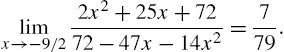
Technically, ![]() does not exist (see Fig. 3.3 (a)) so the following is incorrect.
does not exist (see Fig. 3.3 (a)) so the following is incorrect.
 (Navy blue).
![]()
0
However, using Limit together with the Direction option gives the correct left and right limits.
![]()
∞
![]()
0
We confirm these results by graphing ![]() with Plot in Fig. 3.3 (a). In (b), we also show the graph of
with Plot in Fig. 3.3 (a). In (b), we also show the graph of ![]() in Fig. 3.3 (b), which is further discussed in the exercises.
in Fig. 3.3 (b), which is further discussed in the exercises.
![]()
![]()
![]()
![]()
![]()
![]() □
□
The Limit command together and its options (Direction->1 and Direction->-1) are “fragile” and should be used with caution because the results can be unpredictable. It is wise to check or confirm results using a different technique for nearly all problems encountered.
3.1.4 Continuity
Definition 3.1
The function ![]() is continuous at
is continuous at ![]() if
if
1. ![]() exists;
exists;
2. ![]() exists; and
exists; and
3. ![]() .
.
Note that the third item in the definition means that both (1) and (2) are satisfied. But, if either of (1) or (2) is not satisfied the function is not continuous at the number in question. The function ![]() is continuous on the open interval I if
is continuous on the open interval I if ![]() is continuous at each number a contained in the interval I. Loosely speaking, the “standard” set of functions (polynomials, rational, trigonometric, etc...) are continuous on their domains.
is continuous at each number a contained in the interval I. Loosely speaking, the “standard” set of functions (polynomials, rational, trigonometric, etc...) are continuous on their domains.
Remark 3.3
Be careful with regard to this. For example, since ![]() does not exist, many would say that
does not exist, many would say that ![]() is right continuous at
is right continuous at ![]() .
.
Example 3.6
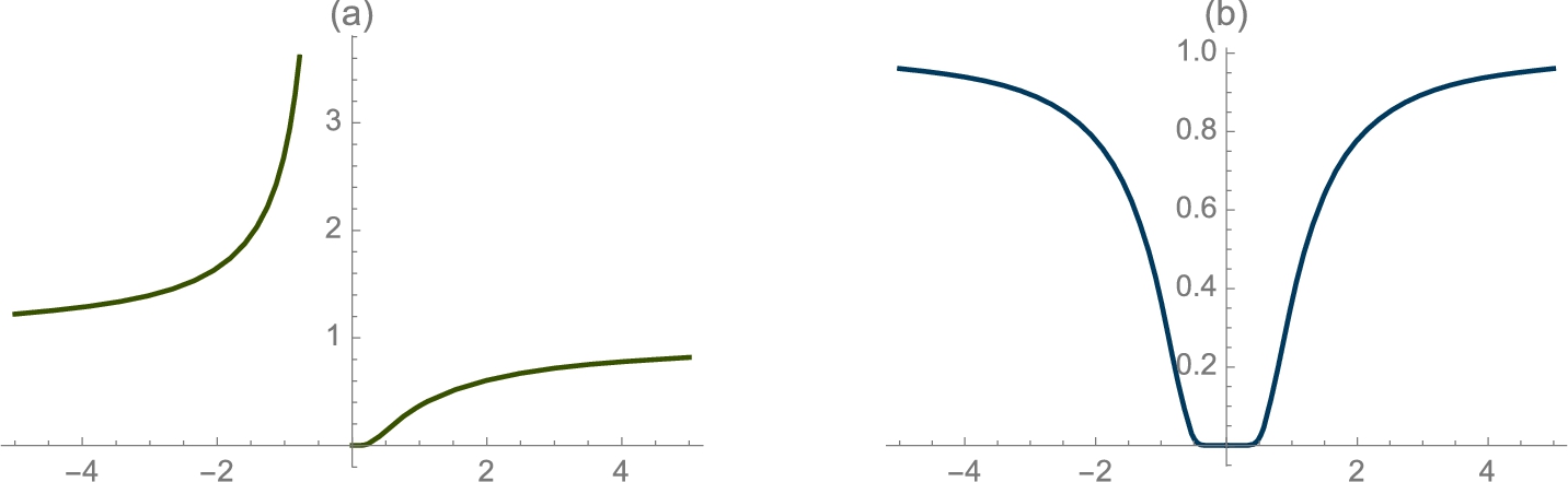
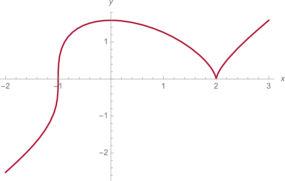
For what value(s) of x, if any, are each of the following functions continuous? (a) ![]() ; (b)
; (b) ![]() ; (c)
; (c) ![]() ; (d)
; (d) ![]() .
.
Solution
(a) Polynomial functions are continuous for all real numbers. In interval notation, ![]() is continuous on
is continuous on ![]() . (b) Because the sine function is continuous for all real numbers,
. (b) Because the sine function is continuous for all real numbers, ![]() is continuous for all real numbers. In interval notation,
is continuous for all real numbers. In interval notation, ![]() is continuous on
is continuous on ![]() . (c) The rational function
. (c) The rational function ![]() is continuous for all
is continuous for all ![]() . In interval notation,
. In interval notation, ![]() is continuous on
is continuous on ![]() . (d)
. (d) ![]() is continuous if the radicand is nonnegative. In interval notation,
is continuous if the radicand is nonnegative. In interval notation, ![]() is strictly continuous on
is strictly continuous on ![]() but some might say that
but some might say that ![]() is continuous on
is continuous on ![]() , where it is understood that
, where it is understood that ![]() is right continuous at
is right continuous at ![]() . We see this by graphing each function with the following commands. See Fig. 3.4. Note that in p3, the vertical line is not a part of the graph of the function—it is a vertical asymptote. If you were to redraw the figure by hand, the vertical line would not be a part of the graph.
. We see this by graphing each function with the following commands. See Fig. 3.4. Note that in p3, the vertical line is not a part of the graph of the function—it is a vertical asymptote. If you were to redraw the figure by hand, the vertical line would not be a part of the graph.
![]()
![]()
![]()
![]()
![]()
![]()
![]()
![]()
![]() □
□
Computers are finite state machines so handling “interesting” functions can be problematic, especially when one must distinguish between rational and irrational numbers. We assume that if ![]() is a rational number (p and q integers),
is a rational number (p and q integers), ![]() is a reduced fraction. One way of tackling these sorts of problems is to view rational numbers as ordered pairs,
is a reduced fraction. One way of tackling these sorts of problems is to view rational numbers as ordered pairs, ![]() . If a and b are integers, Mathematica automatically reduces
. If a and b are integers, Mathematica automatically reduces ![]() so Denominator[a/b] or a/b//Denominator returns the denominator of the reduced fraction; Numerator[a/b] or a/b//Numerator returns the numerator of the reduced fraction. If you want to see the points
so Denominator[a/b] or a/b//Denominator returns the denominator of the reduced fraction; Numerator[a/b] or a/b//Numerator returns the numerator of the reduced fraction. If you want to see the points ![]() for which x is rational, we use ListPlot.
for which x is rational, we use ListPlot.
Example 3.7
Let ![]() . Create a representative graph of
. Create a representative graph of ![]() .
.
Solution
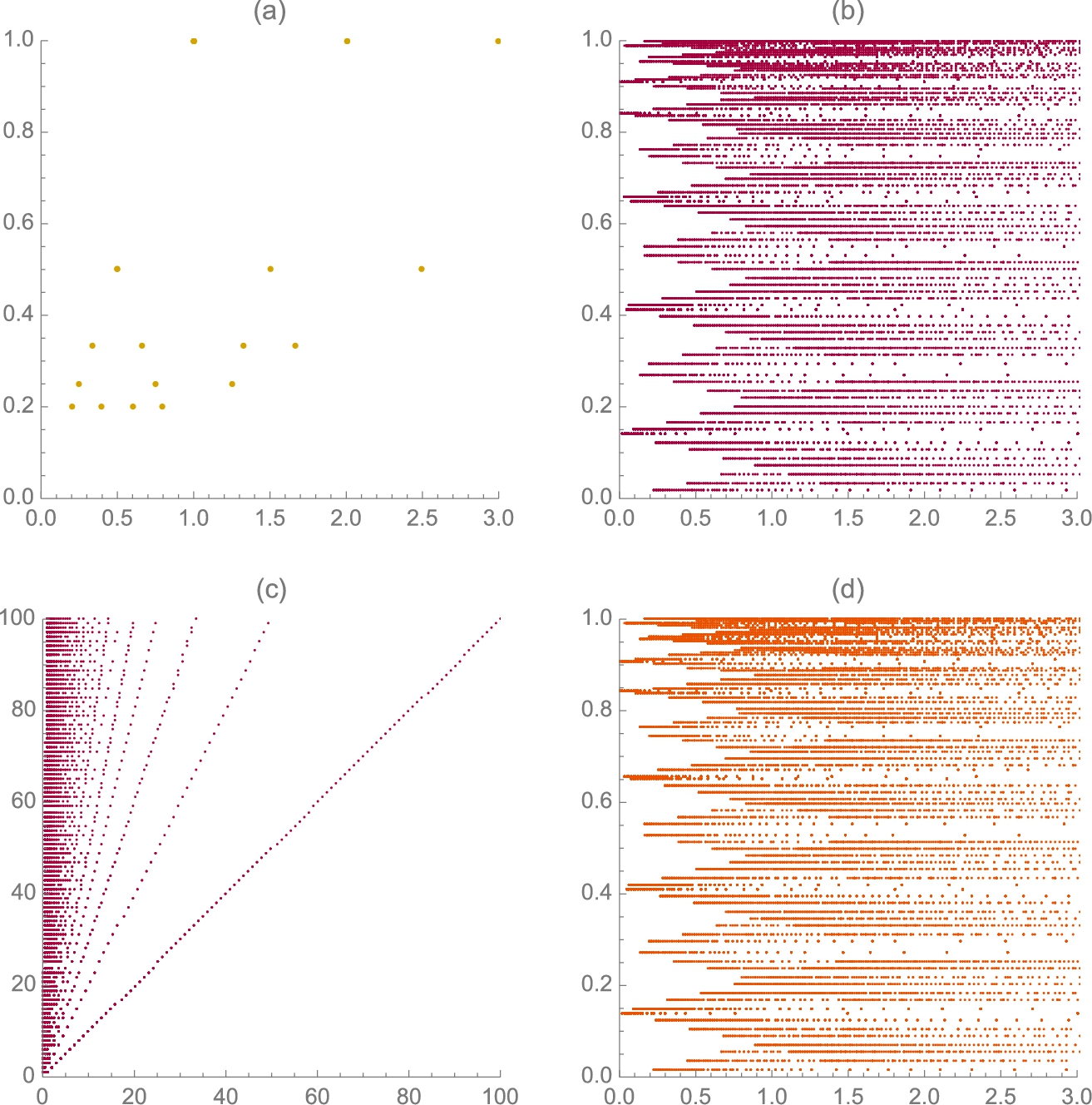
You cannot see points: the measure of the rational numbers is 0, and the measure of the irrational numbers is the continuum, C. A true graph of ![]() would look like the graph of
would look like the graph of ![]() . In the context of the example, we want to see how the graph of
. In the context of the example, we want to see how the graph of ![]() looks for rational values of x. We use a few points to illustrate the technique by using Table and Flatten to generate a set of ordered pairs.
looks for rational values of x. We use a few points to illustrate the technique by using Table and Flatten to generate a set of ordered pairs.
In Mathematica, an ordered pair ![]() is represented by
is represented by ![]() .
.
![]()
![]()
![]()
![]()
![]()
Next, we defined a function f. Assuming that a and b are integers, given an ordered pair ![]() ,
, ![]() returns the point
returns the point ![]()
![]()
We use Map to compute the value of f for each ordered pair in t1. The resulting list is named t2.
![]()
![]()
![]()
![]()
![]()
Notice that t2 contains duplicate entries. We can remove them using Flatten but doing so does not affect the plot shown in Fig. 3.5 (a).
![]()
![]()
![]()
To generate a “prettier” plot, we repeat the procedure using more points. After entering each command the results are not displayed because we include a semicolon (;) at the end of each. See Fig. 3.5 (b).
![]()
![]()
![]()
![]()
![]()
This function is interesting because it is continuous at the irrationals and discontinuous at the rationals.
We can consider other functions in similar contexts. In the following the y-coordinate is the numerator rather than the denominator. See Fig. 3.5 (c).
![]()
![]()
![]()
![]()
![]()
![]()
![]()
With Mathematica, we can modify commands to investigate how changing parameters affect a given situation. In the following, we compute the sine of p if ![]() . See Fig. 3.5 (d).
. See Fig. 3.5 (d).
![]()
![]()
![]()
![]()
![]()
![]()
![]()
![]() □
□
3.2 Differential Calculus
3.2.1 Definition of the Derivative
Definition 3.2
Assuming the derivative exists, as h approaches 0 the secants approach the tangent. Hence, if the limit exists the derivative gives us the slope of a function at that particular value of x.
The Limit command can be used along with Simplify to compute the derivative of a function using the definition of the derivative.
Example 3.8
Use the definition of the derivative to compute the derivative of (a) ![]() , (b)
, (b) ![]() and (c)
and (c) ![]() .
.
Solution
For (a), we first define f, compute the difference quotient, ![]() , simplify the difference quotient with Simplify, and use Limit to calculate the derivative.
, simplify the difference quotient with Simplify, and use Limit to calculate the derivative.
![]()
![]()
![]()
![]()
![]()
![]()
![]()
For (b), we use the same approach as in (a) but use Together rather than Simplify to reduce the complex fraction.
![]()
![]()
![]()
![]()
![]()
![]()
![]()
For (c), observe that Simplify instructs Mathematica to apply elementary trigonometric identities.
![]()
![]()
![]()
![]()
![]()
![]()
![]() □
□
If the derivative of ![]() exists at
exists at ![]() , a geometric interpretation of
, a geometric interpretation of ![]() is that
is that ![]() is the slope of the line tangent to the graph of
is the slope of the line tangent to the graph of ![]() at the point
at the point ![]() .
.
To motivate the definition of the derivative, many calculus texts choose a value of x, ![]() , and then draw the graph of the secant line passing through the points
, and then draw the graph of the secant line passing through the points ![]() and
and ![]() for “small” values of h to show that as h approaches 0, the secant line approaches the tangent line. An equation of the secant line passing through the points
for “small” values of h to show that as h approaches 0, the secant line approaches the tangent line. An equation of the secant line passing through the points ![]() and
and ![]() is given by
is given by

Example 3.9
If ![]() , graph
, graph ![]() together with the secant line containing
together with the secant line containing ![]() and
and ![]() for various values of h.
for various values of h.
Solution
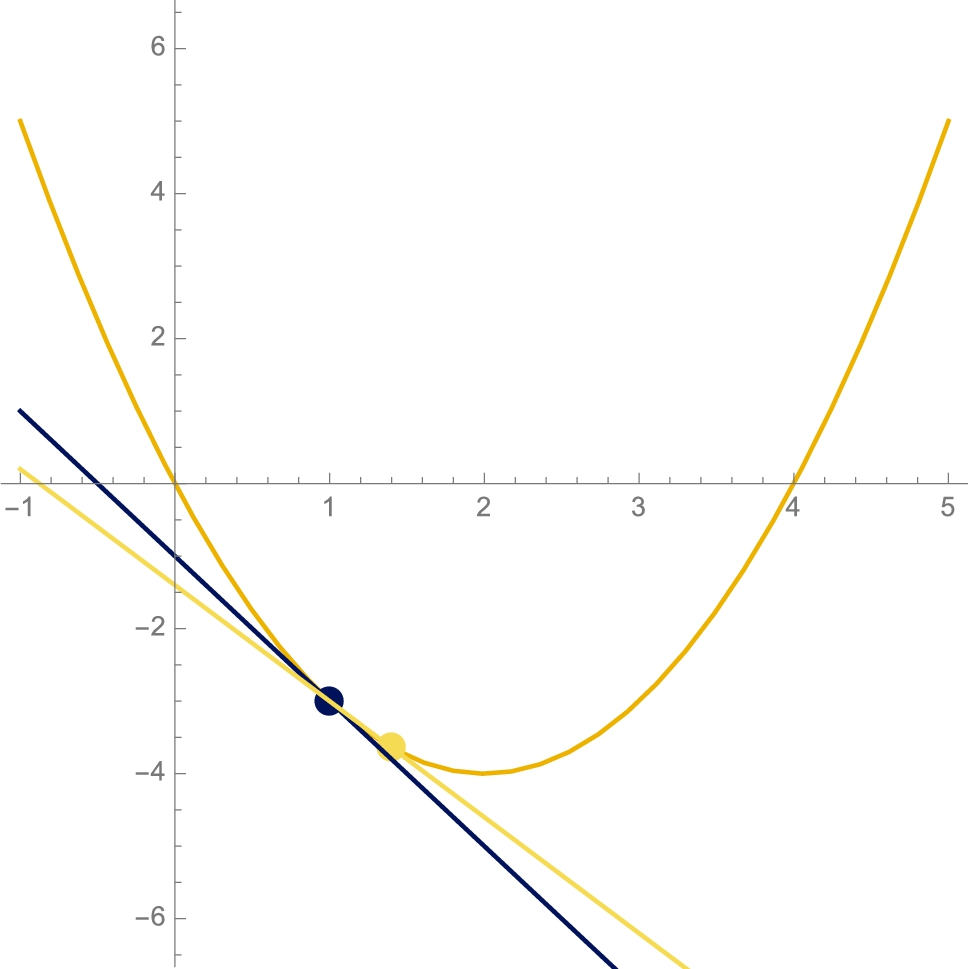
We begin by considering a particular h value. We choose ![]() . We then define
. We then define ![]() . In p1, we graph
. In p1, we graph ![]() in black on the interval
in black on the interval ![]() , in p2 we place a blue point at
, in p2 we place a blue point at ![]() and a green point at
and a green point at ![]() , in p3 we graph the tangent to
, in p3 we graph the tangent to ![]() at
at ![]() in red, in p4 we graph the secant containing
in red, in p4 we graph the secant containing ![]() and
and ![]() in purple, and finally we show all four graphics together with Show in Fig. 3.6.
in purple, and finally we show all four graphics together with Show in Fig. 3.6.
![]()
![]()
![]()
![]()
![]()
![]()
![]()
![]()
We now generalize the previous set of commands for arbitrary ![]() values.
values. ![]() shows plots of
shows plots of ![]() , the tangent at
, the tangent at ![]() , and the secant containing
, and the secant containing ![]() and
and ![]() .
.
![]()
![]()
![]()
![]()
![]()
![]()
![]()
![]()
![]()
![]()
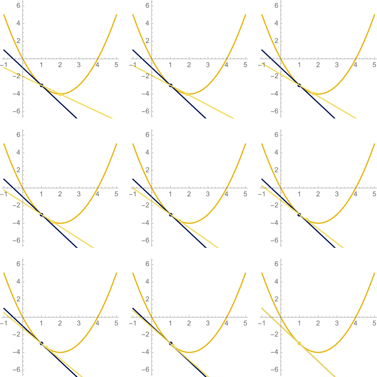
Table[f[x],{x,start,stop,stepsize}] creates a table of ![]() values beginning with
values beginning with ![]() and ending with
and ending with ![]() using increments of
using increments of ![]() . Given a table, Partition[table,n] partitions the table into n element subgroups. Thus if a table, t1 has 9 elements, Partition[t1, 3] creates a
. Given a table, Partition[table,n] partitions the table into n element subgroups. Thus if a table, t1 has 9 elements, Partition[t1, 3] creates a ![]() grid; three sets of three elements each.
grid; three sets of three elements each.
Using Table followed by GraphicsGrid, we can create an table of graphics for various values of h like that shown in Fig. 3.7. With Table, the dimensions of the grid displayed on your computer are based on the size of the active Mathematica window. To control the dimensions of the grid, we use GraphicsGrid together with Partition and Show.
![]()
![]()
Animate works in the same way as Table and is very similar to Manipulate. Entering
![]()
generates an animation of ![]() and 100 equally spaced values of k starting with
and 100 equally spaced values of k starting with ![]() and ending with
and ending with ![]() . To animate the result, use the toolbar in the animate graphic. To vary g continuously and not use a specific stepsize enter Animate[g[k],{k,1,.0001}].
. To animate the result, use the toolbar in the animate graphic. To vary g continuously and not use a specific stepsize enter Animate[g[k],{k,1,.0001}].
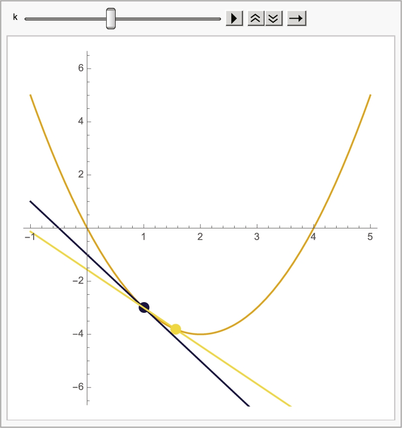
After animating the selection, you can control the animation (speed, direction, pause, and so on) with the buttons at the top of the animation window.
With Mathematica 11, you can use Manipulate to help generate animations and images that you can adjust based on changing parameter values.
To illustrate how to do so, we begin by redefining f and then defining ![]() . Given a and h values,
. Given a and h values, ![]() plots
plots ![]() for
for ![]() (p1), plots a blue point at
(p1), plots a blue point at ![]() and a green point at
and a green point at ![]() (p2), plots
(p2), plots ![]() (the tangent to the graph of
(the tangent to the graph of ![]() at
at ![]() ) for
) for ![]() in red (p3), the secant containing
in red (p3), the secant containing ![]() and
and ![]() for
for ![]() in purple (p4) and finally displays all four graphics together with Show. Using PlotRange, we indicate that horizontal axis displays x values between −10 and 10, the vertical axis displays y values between −10 and 10; AspectRatio->1 means that the ratio of the lengths of the x to y axes is 1. Thus, the plot scaling is correct. Note that when we use Module to define m, p1, p2, p3, and p4 are local to the function m. This means that if you have such objects defined elsewhere in your Mathematica notebook, those objects are not affected when you compute m.
in purple (p4) and finally displays all four graphics together with Show. Using PlotRange, we indicate that horizontal axis displays x values between −10 and 10, the vertical axis displays y values between −10 and 10; AspectRatio->1 means that the ratio of the lengths of the x to y axes is 1. Thus, the plot scaling is correct. Note that when we use Module to define m, p1, p2, p3, and p4 are local to the function m. This means that if you have such objects defined elsewhere in your Mathematica notebook, those objects are not affected when you compute m.
![]()
![]()
![]()
![]()
![]()
![]()
![]()
![]()
![]()
![]()
Now we use Manipulate to create a “mini” program. The sliders (centered at ![]() and
and ![]() with range from −10 to 10 an −1 to 1, respectively) allow you to see how changing a and h affects the plot. See Fig. 3.8.
with range from −10 to 10 an −1 to 1, respectively) allow you to see how changing a and h affects the plot. See Fig. 3.8.
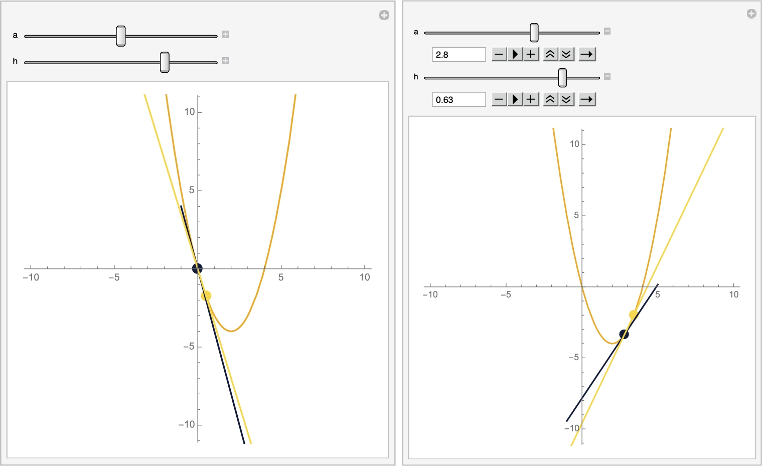
![]()
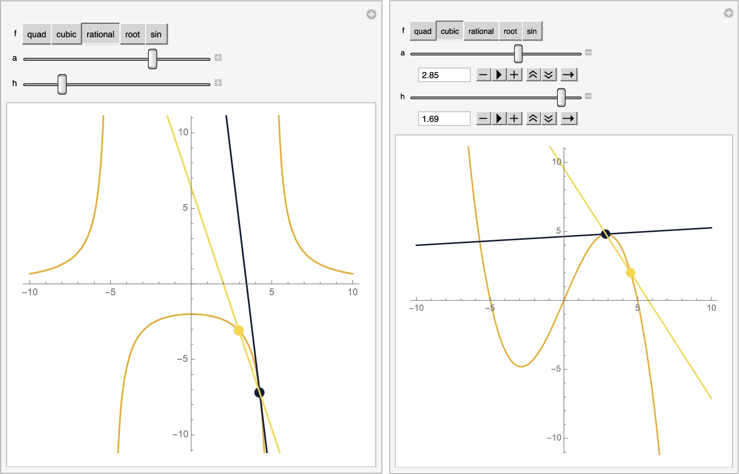
Fig. 3.8 illustrates the special case when ![]() . To illustrate the same concept using a “standard” set of functions (polynomials, rational, root, and trig), we first define the functions
. To illustrate the same concept using a “standard” set of functions (polynomials, rational, root, and trig), we first define the functions
![]()
![]()
![]()
![]()
![]()
and then we adjust m by defining a few of these “standard” and then defining the function mmore, which performs the same actions as m but does so for the function selected. We then use Manipulate to create an object that shows the secant (in yellow), the tangent (in blue) for the selected function, a value, and h value. See Fig. 3.9.
![]()
![]()
![]()
![]()
![]()
![]()
![]()
![]()
![]()
![]()
![]() □
□
3.2.2 Calculating Derivatives
The functions D and ' are used to differentiate functions. Assuming that ![]() is differentiable,
is differentiable,
1. D[f[x],x] computes and returns ![]() ,
,
2. f'[x] computes and returns ![]() ,
,
3. f''[x] computes and returns ![]() , and
, and
4. D[f[x],{x,n}] computes and returns ![]() .
.
5. You can use the ![]() button located on the Basic Math Assistant and Basic Math Input palettes to create templates to compute derivatives.
button located on the Basic Math Assistant and Basic Math Input palettes to create templates to compute derivatives.
Fig. 3.10 illustrates various ways of computing derivatives using the ′ symbol, D, and the ∂ symbol.
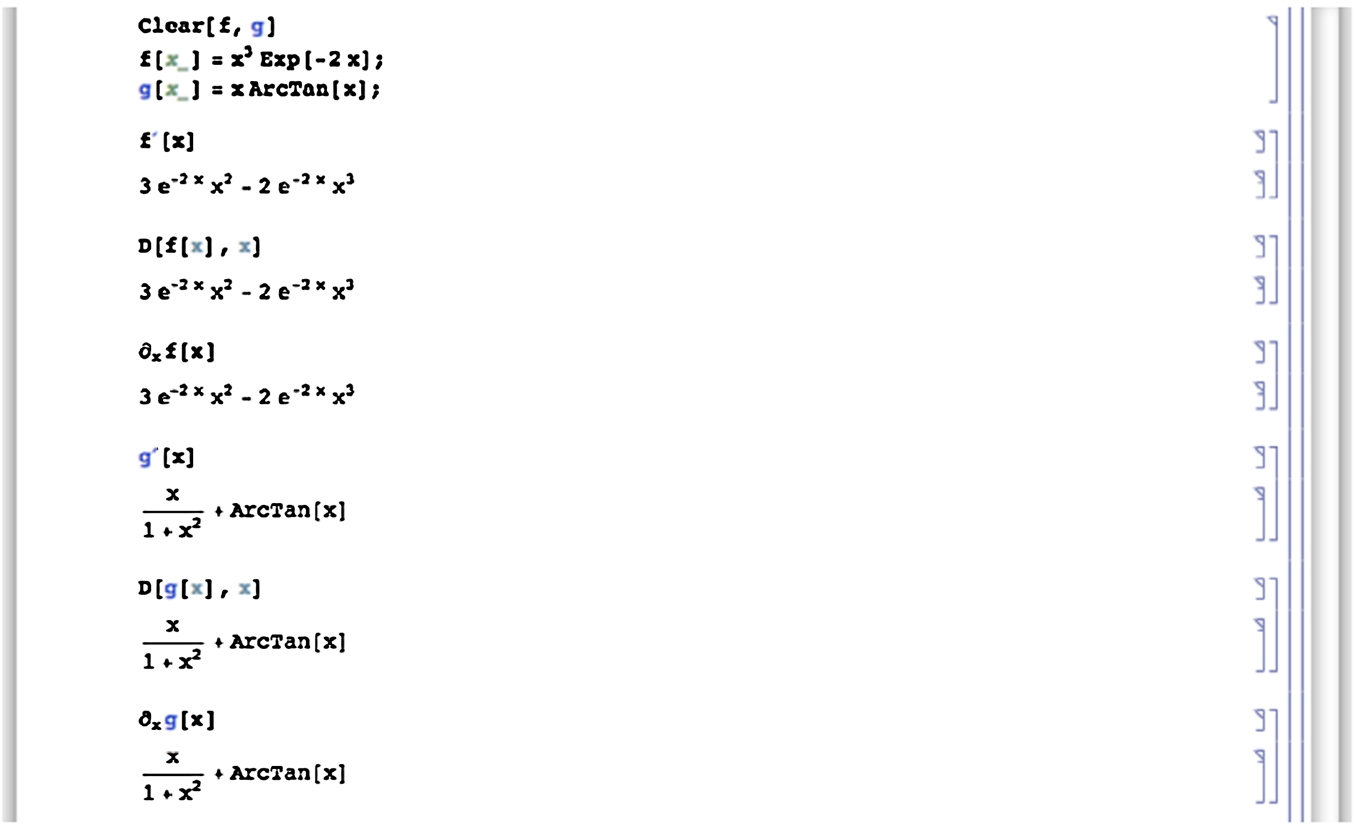
Mathematica knows the numerous differentiation rules, including the product, quotient, and chain rules. Thus, entering
![]()
![]()
![]()
shows us that ![]() ; entering
; entering
![]()
![]()
shows us that
Remark 3.4
Throughout the text, input is in Bold and output is Not; output follows input ![]() ; and entering
; and entering
![]()
![]()
shows us that ![]() .
.
Example 3.10
Compute the first and second derivatives of (a) ![]() , (b)
, (b) ![]() , (c)
, (c) ![]() , and (d)
, and (d) ![]() .
.
Solution
For (a), we use D.
![]()
![]()
For (b), we first define f and then use ′ together with Factor to calculate and factor ![]() and
and ![]() .
.
![]()
![]()
![]()
![]()
![]()
For (c), we use Simplify together with D to calculate and simplify ![]() and
and ![]() .
.
![]()
![]()
![]()
![]()
By hand, (d) would require logarithmic differentiation. The second derivative would be particularly difficult to compute by hand. Mathematica quickly computes and simplifies each derivative.
![]()
![]()
![]()
![]() □
□
The command Map[f,list] applies the function f to each element of the list list. Thus, if you are computing the derivatives of a large number of functions, you can use Map together with D.
A built-in Mathematica function is threadable if f[list] returns the same result as Map[f,list]. Many familiar functions like D and Integrate are threadable.
Example 3.11
Compute the first and second derivatives of ![]() ,
, ![]() ,
, ![]() ,
, ![]() ,
, ![]() , and
, and ![]() .
.
Solution
Notice that lists are contained in braces. Thus, entering
![]()
![]()
![]()
computes the first derivative of the three trigonometric functions and their inverses. In this case, we have applied a pure function to the list of trigonometric functions and their inverses. Given an argument #, D[#,x]& computes the derivative of # with respect to x. The & symbol is used to mark the end of a pure function. Similarly, entering
![]()
![]()
![]()
computes the second derivative of the three trigonometric functions and their inverses. Because D is threadable, the same results are obtained with the following commands.
![]()
![]()
![]()
![]()
![]()
![]() □
□
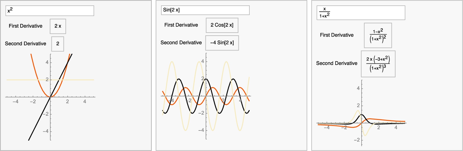
With DynamicModule, we create a simple dynamic that lets you compute the first and second derivatives of basic functions and plot them on a standard viewing window, ![]() . The layout of Fig. 3.11 is primarily determined by Panel, Column, and Grid. The default function is
. The layout of Fig. 3.11 is primarily determined by Panel, Column, and Grid. The default function is ![]() . To compute and graph the first and second derivatives of a different function, simply type over
. To compute and graph the first and second derivatives of a different function, simply type over ![]() with the desired function.
with the desired function.
![]()
![]()
![]()
![]()
![]()
![]()
![]()
![]()
3.2.3 Implicit Differentiation
If an equation contains two variables, x and y, implicit differentiation can be carried out by explicitly declaring y to be a function of x, ![]() , and using D or by using the Dt command.
, and using D or by using the Dt command.
Example 3.12
Find ![]() if (a)
if (a) ![]() and (b)
and (b) ![]() .
.
Solution
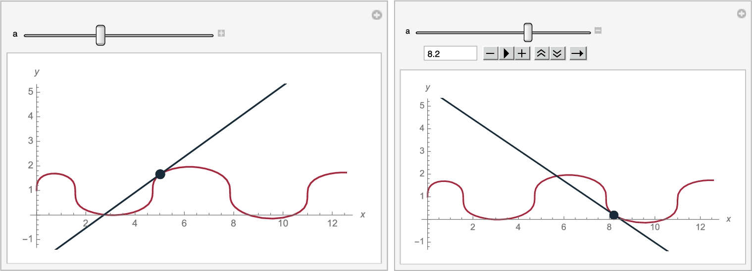
For (a) we illustrate the use of D. Notice that we are careful to specifically indicate that ![]() . First we differentiate with respect to x
. First we differentiate with respect to x
![]()
![]()
![]() and then we solve the resulting equation for
and then we solve the resulting equation for ![]() with Solve.
with Solve.
![]()
![]()
For (b), we use Dt. When using Dt, we interpret Dt[x]=1 and Dt[y]![]() . Thus, entering
. Thus, entering
![]()
![]()
![]()
![]()
and solving for dydx with Solve
![]()
![]()
shows us that if ![]() ,
, ![]() .
.
To graph each equation, we use ContourPlot. Generally, given an equation of the form ![]() , the command
, the command
ContourPlot[f[x,y]==g[x,y],{x,a,b},{y,c,d}]
attempts to plot the graph of ![]() on the rectangle
on the rectangle ![]() . Using Show together with GraphicsRow, we show the two graphs side-by-side in Fig. 3.12.
. Using Show together with GraphicsRow, we show the two graphs side-by-side in Fig. 3.12.
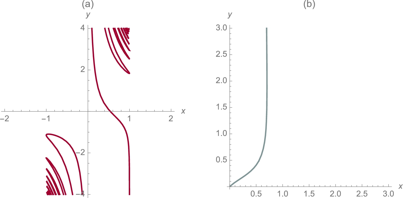
 for −2 ⩽ x ⩽ 2 and −4 ⩽ y ⩽ 4; on the right,
  for .01 ⩽ x ⩽ 3 and .01 ⩽ y ⩽ 3 (MIT colors).
![]()
![]()
![]()
![]()
![]()
![]()
![]()
![]()
![]() □
□
3.2.4 Tangent Lines
If ![]() exists,
exists, ![]() is interpreted to be the slope of the line tangent to the graph of
is interpreted to be the slope of the line tangent to the graph of ![]() at the point
at the point ![]() . In this case, an equation of the tangent is given by
. In this case, an equation of the tangent is given by
Example 3.13
Find an equation of the line tangent to the graph of ![]() at the point with x-coordinate
at the point with x-coordinate ![]() .
.
Solution
Recall that when computing odd roots of negative numbers, Mathematica returns the value with the largest imaginary part. However, for our purposes, we need the real-valued root. To obtain the real-valued root, use Surd: Surd[x,n] returns the real-valued root of x if n is odd. Because we will be graphing a function involving odd roots of negative numbers, we define ![]() using the Surd function and then compute
using the Surd function and then compute ![]() .
.
![]()
![]()
![]()
Then, the slope of the line tangent to the graph of ![]() at the point with x-coordinate
at the point with x-coordinate ![]() is
is
![]()
![]()
![]()
0.440013
while the y-coordinate of the point is
![]()
![]()
![]()
1.78001
Thus, an equation of the line tangent to the graph of ![]() at the point with x-coordinate
at the point with x-coordinate ![]() is
is

as shown in Fig. 3.13.
 together with its tangent at the point
 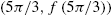 (Stanford colors).
![]()
![]()
![]()
![]()
![]()
![]()
![]()
We use Manipulate to plot different tangents or animate the tangents as shown in Fig. 3.14.
![]()
![]()
![]()
![]()
![]()
![]()
![]() □
□
Remark 3.5
Sometimes using Surd may be cumbersome. Therefore, it is worth noting that if you desire a real root to ![]() and there is a real root, x^(n/m)=Abs[x]^(n/m) if n is even and x^(n/m)=Sign[x]Abs[x]^(n/m) if n is odd. Of course, remember that if m is even and x is negative,
and there is a real root, x^(n/m)=Abs[x]^(n/m) if n is even and x^(n/m)=Sign[x]Abs[x]^(n/m) if n is odd. Of course, remember that if m is even and x is negative, ![]() is not a real number. Note that Sign[x] returns 1 if x is positive and −1 if x is negative.
is not a real number. Note that Sign[x] returns 1 if x is positive and −1 if x is negative.
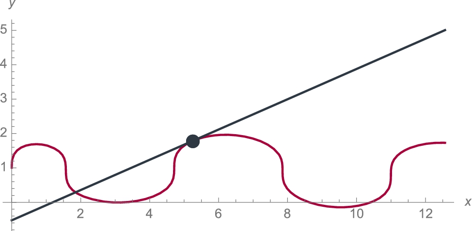
Tangent Lines of Implicit Functions
Example 3.14
Find equations of the tangent line and normal line to the graph of ![]() at the point
at the point ![]() . Find and simplify
. Find and simplify ![]() .
.
If the line ℓ has slope ![]() the line perpendicular (or, normal) to ℓ has slope
the line perpendicular (or, normal) to ℓ has slope ![]() .
.
Solution
We evaluate ![]() if
if ![]() and
and ![]() to determine the slope of the tangent line at the point
to determine the slope of the tangent line at the point ![]() . Note that we cannot (easily) solve
. Note that we cannot (easily) solve ![]() for y so we use implicit differentiation to find
for y so we use implicit differentiation to find ![]() :
:
By the product and chain rules, ![]() .
.
![]()
![]()
![]()
![]()
![]()
![]()
![]()
![]()
Notice that s3 is a list. The formula for ![]() is the second part of the first part of the first part of s3 and extracted from s3 with
is the second part of the first part of the first part of s3 and extracted from s3 with
![]()
![]()
We then use ReplaceAll (/.) to find that the slope of the tangent at ![]() is
is
![]()
1
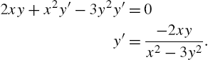
The slope of the normal is ![]() . Equations of the tangent and normal are given by
. Equations of the tangent and normal are given by
respectively. See Fig. 3.15.
![]()
![]()
![]()
![]()
![]()
![]()
![]()
![]()
To find ![]() , we proceed as follows.
, we proceed as follows.
![]()
![]()
![]()
![]()
The result means that

Because ![]() , the second derivative is further simplified to
, the second derivative is further simplified to

□
Parametric Equations and Polar Coordinates
For the parametric equations ![]() ,
, ![]() ,
,
and

If ![]() has a tangent line at the point
has a tangent line at the point ![]() , parametric equations of the tangent are given by
, parametric equations of the tangent are given by
If ![]() ,
, ![]() , we can eliminate the parameter from (3.2)
, we can eliminate the parameter from (3.2)
and obtain an equation of the tangent line in point-slope form.
![]()
![]()
![]()
![]()
Example 3.15
The Cycloid
Solution
After defining x and y we use ' to compute ![]() and
and ![]() . We then compute
. We then compute ![]() and
and ![]() .
.
![]()
![]()
![]()
![]()
![]()
![]()
![]()
![]()
![]()
![]()
![]()
![]()
We then use ParametricPlot to graph the cycloid for ![]() , naming the resulting graph p1.
, naming the resulting graph p1.
![]()
![]()
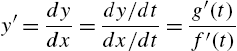
Next, we use Table to define toplot to be 40 tangent lines (3.2) using equally spaced values of a between ![]() and 4π. We then graph each line toplot and name the resulting graph p2. Finally, we show p1 and p2 together with the Show function. The resulting plot is shown to scale because the lengths of the x and y-axes are equal and we include the option AspectRatio->1. In the graphs, notice that on intervals for which
and 4π. We then graph each line toplot and name the resulting graph p2. Finally, we show p1 and p2 together with the Show function. The resulting plot is shown to scale because the lengths of the x and y-axes are equal and we include the option AspectRatio->1. In the graphs, notice that on intervals for which ![]() is defined,
is defined, ![]() is a decreasing function and, consequently,
is a decreasing function and, consequently, ![]() . (See Fig. 3.16.)
. (See Fig. 3.16.)
![]()
![]()
![]()
![]()
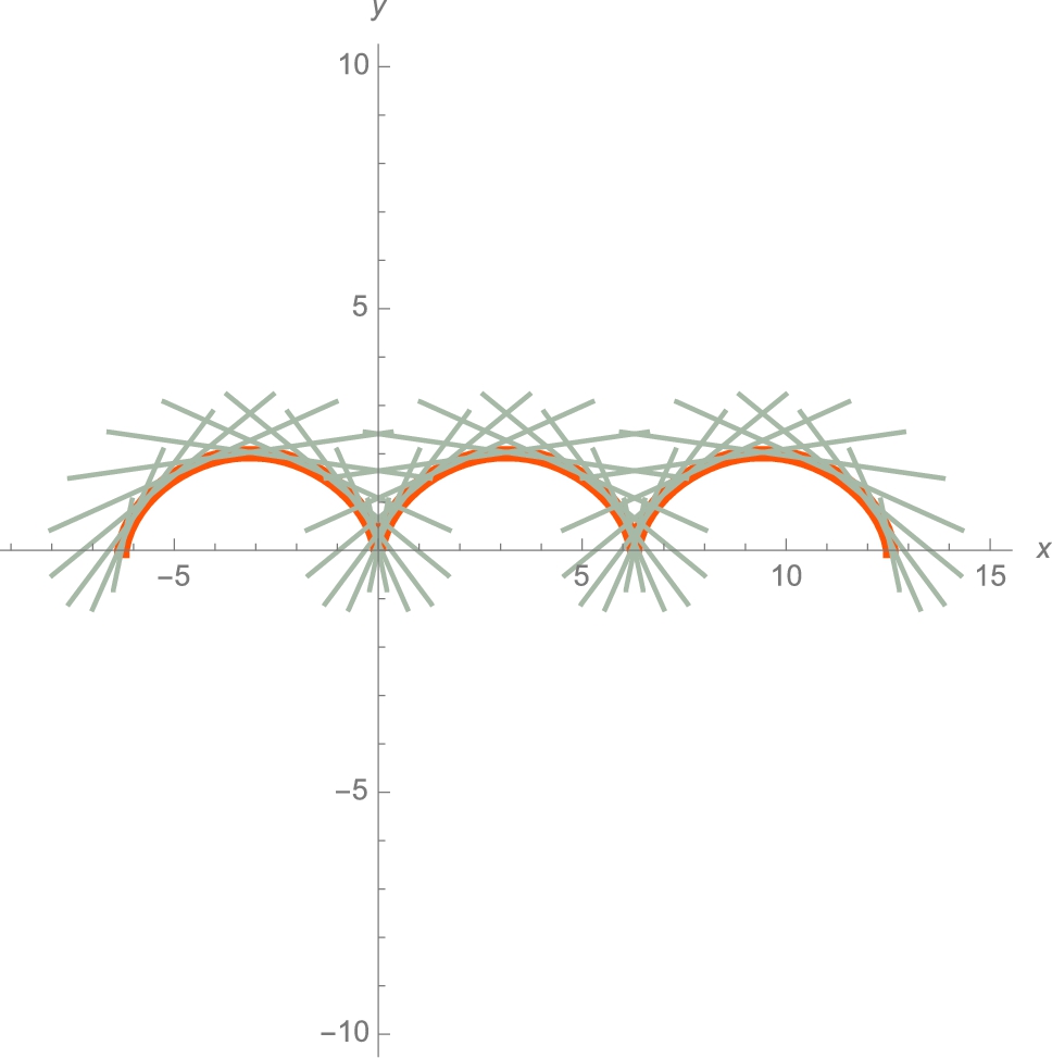
With Manipulate, you can animate the tangents. (See Fig. 3.17.)
![]()
![]()
![]()
![]()
![]()
![]()
![]()
![]() □
□
Example 3.16
Orthogonal Curves
Two lines ![]() and
and ![]() with slopes
with slopes ![]() and
and ![]() , respectively, are orthogonal if their slopes are negative reciprocals:
, respectively, are orthogonal if their slopes are negative reciprocals: ![]() .
.
Extended to curves, we say that the curves ![]() and
and ![]() are orthogonal at a point of intersection if their respective tangent lines to the curves at that point are orthogonal.
are orthogonal at a point of intersection if their respective tangent lines to the curves at that point are orthogonal.
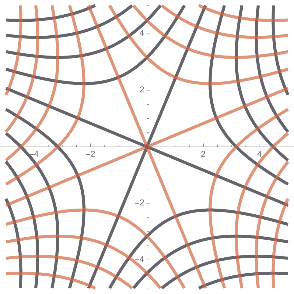
Show that the family of curves with equation ![]() is orthogonal to the family of curves with equation
is orthogonal to the family of curves with equation ![]() .
.
Solution
We begin by defining eq1 and eq2 to be equations ![]() and
and ![]() , respectively. Then, use Dt to differentiate and Solve to find
, respectively. Then, use Dt to differentiate and Solve to find ![]() .
.
![]()
![]()
![]()
![]()
![]()
![]()
Because the derivatives are negative reciprocals, we conclude that the curves are orthogonal. We confirm this graphically by graphing several members of each family with ContourPlot and showing the results together. (See Fig. 3.18.)
![]()
![]()
![]()
![]()
![]() □
□
Theorem 3.1
The Mean-Value Theorem for Derivatives
Example 3.17
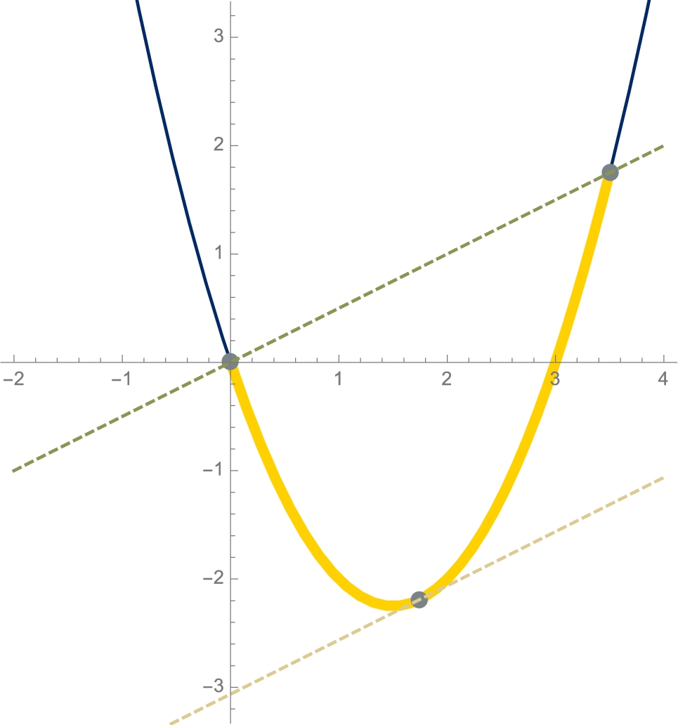
Find all number(s) c that satisfy the conclusion of the Mean-Value Theorem for ![]() on the interval
on the interval ![]() .
.
Solution
By the power rule, ![]() . The slope of the secant containing
. The slope of the secant containing ![]() and
and ![]() is
is

Solving ![]() for x gives us
for x gives us ![]() .
.
![]()
![]()
![]()
![]()
![]()
![]()
![]() satisfies the conclusion of the Mean-Value Theorem for
satisfies the conclusion of the Mean-Value Theorem for ![]() on the interval
on the interval ![]() , as shown in Fig. 3.19.
, as shown in Fig. 3.19.
![]()
![]()
![]()
![]()
![]()
![]()
![]()
![]()
![]() □
□
3.2.5 The First Derivative Test and Second Derivative Test
Example 3.15 illustrates the following properties of the first and second derivative.
Theorem 3.2
Let ![]() be continuous on
be continuous on ![]() and differentiable on
and differentiable on ![]() .
.
1. If ![]() for all x in
for all x in ![]() , then
, then ![]() is constant on
is constant on ![]() .
.
2. If ![]() for all x in
for all x in ![]() , then
, then ![]() is increasing on
is increasing on ![]() .
.
3. If ![]() for all x in
for all x in ![]() , then
, then ![]() is decreasing on
is decreasing on ![]() .
.
For the second derivative, we have the following theorem.
Theorem 3.3
Let ![]() have a second derivative on
have a second derivative on ![]() .
.
1. If ![]() for all x in
for all x in ![]() , then the graph of
, then the graph of ![]() is concave up on
is concave up on ![]() .
.
2. If ![]() for all x in
for all x in ![]() , then the graph of
, then the graph of ![]() is concave down on
is concave down on ![]() .
.
The critical points correspond to those points on the graph of ![]() where the tangent line is horizontal or vertical; the number
where the tangent line is horizontal or vertical; the number ![]() is a critical number if
is a critical number if ![]() or
or ![]() does not exist if
does not exist if ![]() . The inflection points correspond to those points on the graph of
. The inflection points correspond to those points on the graph of ![]() where the graph of
where the graph of ![]() is neither concave up nor concave down. Theorems 3.2 and 3.3 help establish the first derivative test and second derivative test.
is neither concave up nor concave down. Theorems 3.2 and 3.3 help establish the first derivative test and second derivative test.
Theorem 3.4
First Derivative Test
Let ![]() be a critical number of a function
be a critical number of a function ![]() continuous on an open interval I containing
continuous on an open interval I containing ![]() . If
. If ![]() is differentiable on I, except possibly at
is differentiable on I, except possibly at ![]() ,
, ![]() can be classified as follows.
can be classified as follows.
1. If ![]() makes a simple change in sign from positive to negative at
makes a simple change in sign from positive to negative at ![]() , then
, then ![]() is a relative maximum.
is a relative maximum.
2. If ![]() makes a simple change in sign from negative to positive at
makes a simple change in sign from negative to positive at ![]() , then
, then ![]() is a relative minimum.
is a relative minimum.
Theorem 3.5
Second Derivative Test
Let ![]() be a critical number of a function
be a critical number of a function ![]() and suppose that
and suppose that ![]() exists on an open interval containing
exists on an open interval containing ![]() .
.
1. If ![]() , then
, then ![]() is a relative maximum.
is a relative maximum.
2. If ![]() , then
, then ![]() is a relative minimum.
is a relative minimum.
Example 3.18
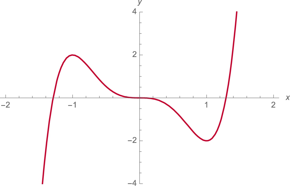
Graph ![]() .
.
Solution
We begin by defining ![]() and then computing and factoring
and then computing and factoring ![]() and
and ![]() .
.
![]()
![]()
![]()
![]()
![]()
By inspection, we see that the critical numbers are ![]() , 1, and −1 while
, 1, and −1 while ![]() if
if ![]() ,
, ![]() , or
, or ![]() . Of course, these values can also be found with Solve as done next in cns and ins, respectively.
. Of course, these values can also be found with Solve as done next in cns and ins, respectively.
![]()
![]()
![]()
![]()
We find the critical and inflection points by using /. (Replace All) to compute ![]() for each value of x in cns and ins, respectively. The result means that the critical points are
for each value of x in cns and ins, respectively. The result means that the critical points are ![]() ,
, ![]() and
and ![]() ; the inflection points are
; the inflection points are ![]() ,
, ![]() , and
, and ![]() . We also see that
. We also see that ![]() so Theorem 3.5 cannot be used to classify
so Theorem 3.5 cannot be used to classify ![]() . On the other hand,
. On the other hand, ![]() and
and ![]() so by Theorem 3.5,
so by Theorem 3.5, ![]() is a relative minimum and
is a relative minimum and ![]() is a relative maximum.
is a relative maximum.
![]()
![]()
![]()
![]()
![]()
![]()
We can graphically determine the intervals of increase and decrease by noting that if ![]() (
(![]() ),
), ![]() (
(![]() ). Similarly, the intervals for which the graph is concave up and concave down can be determined by noting that if
). Similarly, the intervals for which the graph is concave up and concave down can be determined by noting that if ![]() (
(![]() ),
), ![]() (
(![]() ). We use Plot to graph
). We use Plot to graph ![]() and
and ![]() (different values are used so we can differentiate between the two plots) in Fig. 3.20.
(different values are used so we can differentiate between the two plots) in Fig. 3.20.
![]()
![]()
From the graph, we see that ![]() for x in
for x in ![]() ,
, ![]() for x in
for x in ![]() ,
, ![]() for x in
for x in ![]() , and
, and ![]() for x in
for x in ![]() . Thus, the graph of
. Thus, the graph of ![]() is
is
• increasing and concave down for x in ![]() ,
,
• decreasing and concave down for x in ![]() ,
,
• decreasing and concave up for x in ![]() ,
,
• decreasing and concave down for x in ![]() ,
,
• decreasing and concave up for x in ![]() , and
, and
• increasing and concave up for x in ![]() .
.
We also see that ![]() is neither a relative minimum nor maximum. To see all points of interest, our domain must contain −1 and 1 while our range must contain −2 and 2. We choose to graph
is neither a relative minimum nor maximum. To see all points of interest, our domain must contain −1 and 1 while our range must contain −2 and 2. We choose to graph ![]() for
for ![]() ; we choose the range displayed to be
; we choose the range displayed to be ![]() . (See Fig. 3.21.)
. (See Fig. 3.21.)
![]()
![]()
![]() □
□
Remember to be especially careful when working with functions that involve odd roots. If n is odd and x is even, use Surd[x,n] to obtain the real-valued nth root of x.
Example 3.19
Graph ![]() .
.
Solution
We begin by defining ![]() and then computing and simplifying
and then computing and simplifying ![]() and
and ![]() with ′ and Simplify.
with ′ and Simplify.
![]()
![]()
![]()
![]()
![]()
![]()
By inspection, we see that the critical numbers are ![]() , 2, and −1. We cannot use Theorem 3.5 to classify
, 2, and −1. We cannot use Theorem 3.5 to classify ![]() and
and ![]() because
because ![]() is undefined if
is undefined if ![]() or −1. On the other hand,
or −1. On the other hand, ![]() so
so ![]() is a relative maximum. By hand, we make a sign chart to see that the graph of
is a relative maximum. By hand, we make a sign chart to see that the graph of ![]() is
is
• increasing and concave up on ![]() ,
,
• increasing and concave down on ![]() ,
,
• decreasing and concave down on ![]() , and
, and
• increasing and concave down on ![]() .
.
Hence, ![]() is neither a relative minimum nor maximum while
is neither a relative minimum nor maximum while ![]() is a relative minimum by Theorem 3.4. We use Plot to graph
is a relative minimum by Theorem 3.4. We use Plot to graph ![]() for
for ![]() in Fig. 3.22.
in Fig. 3.22.
![]()
![]()
![]()
![]()
![]() □
□
The previous examples illustrate that if ![]() is a critical number of
is a critical number of ![]() and
and ![]() makes a simple change in sign from positive to negative at
makes a simple change in sign from positive to negative at ![]() , then
, then ![]() is a relative maximum. If
is a relative maximum. If ![]() makes a simple change in sign from negative to positive at
makes a simple change in sign from negative to positive at ![]() , then
, then ![]() is a relative minimum. Mathematica is especially useful in investigating interesting functions for which this may not be the case.
is a relative minimum. Mathematica is especially useful in investigating interesting functions for which this may not be the case.
Example 3.20
Consider
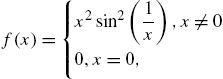
![]() is a critical number because
is a critical number because ![]() does not exist if
does not exist if ![]() . The point
. The point ![]() is both a relative and absolute minimum, even though
is both a relative and absolute minimum, even though ![]() does not make a simple change in sign at
does not make a simple change in sign at ![]() , as illustrated in Fig. 3.23.
, as illustrated in Fig. 3.23.
 and f′(x) for −0.1 ⩽ x ⩽ 0.1 (Carnegie Mellon colors).
![]()
![]()
![]()
![]()
![]()
![]()
![]()
![]()
![]()
![]()
Notice that the derivative “oscillates” infinitely many times near ![]() , so the first derivative test cannot be used to classify
, so the first derivative test cannot be used to classify ![]() .
.
The functions Maximize and Minimize can be used to assist with finding extreme values. For a function of a single variable Maximize[f[x],x] (Minimize[f[x],x]) attempts to find the maximum (minimum) values of ![]() ; Maximize[{f[x],a<=x<=b},x] (Minimize[{f[x],a<=x<=b},x]) attempts to find the maximum (minimum) values of
; Maximize[{f[x],a<=x<=b},x] (Minimize[{f[x],a<=x<=b},x]) attempts to find the maximum (minimum) values of ![]() on
on ![]() .
.
Example 3.21
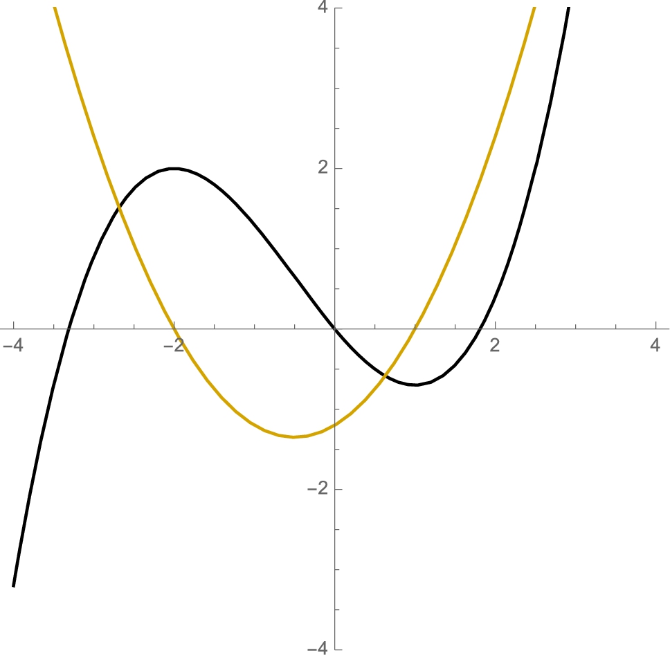
Consider ![]() . After defining
. After defining ![]() , we plot
, we plot ![]() and
and ![]() together in Fig. 3.24.
together in Fig. 3.24.
![]()
![]()
![]()
With Maximize, we see that ![]() does not have a maximum on its domain. However, when we restrict the interval to
does not have a maximum on its domain. However, when we restrict the interval to ![]() , Maximize finds the relative maximum at
, Maximize finds the relative maximum at ![]() .
.
![]()
![]()
![]()
![]()
![]()
Similarly, with Minimize we see that the ![]() does not have a minimum value on its domain but find the relative minimum when we restrict the interval to
does not have a minimum value on its domain but find the relative minimum when we restrict the interval to ![]() .
.
![]()
![]()
![]()
![]()
![]()
However, with Solve, we easily find the two zeros of ![]() that we see in Fig. 3.24
that we see in Fig. 3.24
![]()
![]()
When using Maximize or Minimize you should verify your results using another method.
Example 3.22
The function ![]() is continuous on
is continuous on ![]() and
and ![]() . Thus,
. Thus, ![]() has an absolute minimum and maximum value on its domain. In this case,
has an absolute minimum and maximum value on its domain. In this case,
![]()
![]()
![]()
![]()
gives us the absolute maximum and minimum values of ![]() and the x-values where they occur. On the other hand,
and the x-values where they occur. On the other hand, ![]() is continuous on
is continuous on ![]() and
and ![]() . Thus,
. Thus, ![]() has an absolute minimum on its domain. Because the derivative of a fourth degree polynomial is a third degree polynomial, we know that
has an absolute minimum on its domain. Because the derivative of a fourth degree polynomial is a third degree polynomial, we know that ![]() has three zeros, two of which probably correspond to relative minimums. Because the graph of
has three zeros, two of which probably correspond to relative minimums. Because the graph of ![]() is symmetric with respect to the y-axis, we further suspect that the absolute minimum is obtained twice—at each relative minimum. Maximize and Minimize give us the following results.
is symmetric with respect to the y-axis, we further suspect that the absolute minimum is obtained twice—at each relative minimum. Maximize and Minimize give us the following results.
![]()
![]()
![]()
![]()
![]()
Note that the result returned by Maximize is correct. Similarly, the result returned by Minimize is correct, but a complete answer would indicate that the absolute minimum value occurs at both ![]() and
and ![]() .
.
Example 3.23
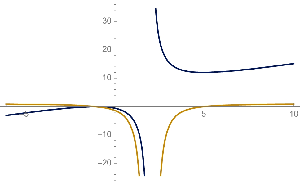
The function ![]() has a vertical asymptote at
has a vertical asymptote at ![]() . From the derivative,
. From the derivative,
![]()
![]()
![]()
![]()
![]()
![]()
![]()
we find two critical numbers, one of which is a relative maximum and one is a relative minimum. See Fig. 3.25.
![]()
![]()
![]()
On the other hand, Maximize and Minimize return confusing results because the function is undefined if ![]() . The function has relative extreme values but not absolute extreme values.
. The function has relative extreme values but not absolute extreme values.
![]()
![]()
![]()
![]()
![]()
![]()
From the graph in Fig. 3.25, we see that ![]() while
while ![]() .
.
For periodic functions, such as sine and cosine, Maximize and Minimize generally don't indicate all extreme values.
![]()
![]()
![]()
![]()
3.2.6 Applied Max/Min Problems
Mathematica can be used to assist in solving maximization/minimization problems encountered in a differential calculus course.
Example 3.24
A woman is located on one side of a body of water 4 miles wide. Her position is directly across from a point on the other side of the body of water 16 miles from her house, as shown in the following figure.
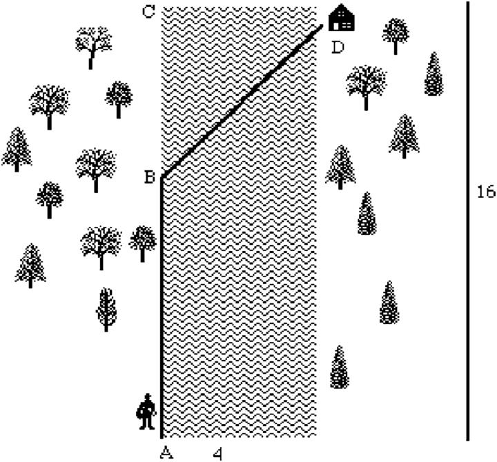
If she can move across land at a rate of 10 miles per hour and move over water at a rate of 6 miles per hour, find the least amount of time for her to reach her house.
Solution
From the figure, we see that the woman will travel from A to B by land and then from B to D by water. We wish to find the least time for her to complete the trip.
Let x denote the distance BC, where ![]() . Then, the distance AB is given by
. Then, the distance AB is given by ![]() and, by the Pythagorean theorem, the distance BD is given by
and, by the Pythagorean theorem, the distance BD is given by ![]() . Because
. Because ![]() ,
, ![]() . Thus, the time to travel from A to B is
. Thus, the time to travel from A to B is ![]() , the time to travel from B to D is
, the time to travel from B to D is ![]() , and the total time to complete the trip, as a function of x, is
, and the total time to complete the trip, as a function of x, is
We must minimize the function ![]() . First, we define time and then verify that time has a minimum by graphing time on the interval
. First, we define time and then verify that time has a minimum by graphing time on the interval ![]() in Fig. 3.26.
in Fig. 3.26.
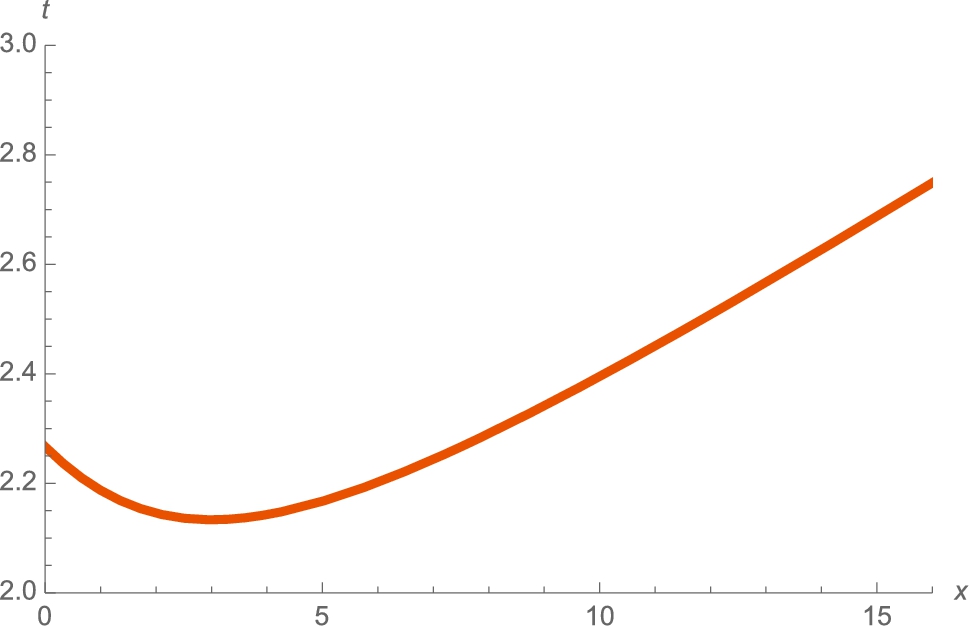
 , 0 ⩽ x ⩽ 16 (The University of Texas at Austin colors).
![]()
![]()
![]()
![]()
![]()
Next, we compute the derivative of time and find the values of x for which the derivative is 0 with Solve. The resulting output is named critnums using ReplaceAll (\.).
![]()
![]()
![]()
![]()
At this point, we can calculate the minimum time by calculating time[3].
![]()
![]()
Alternatively, we demonstrate how to find the value of time[x] for the value(s) listed in critnums.
![]()
![]()
Regardless, we see that the minimum time to complete the trip is 32/15 hours. □
One of the more interesting applied max/min problems is the beam problem. We present two solutions.
Example 3.25
The Beam Problem
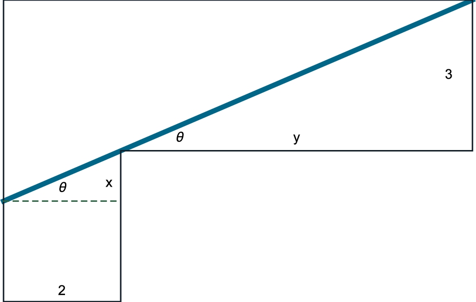
Find the exact length of the longest beam that can be carried around a corner from a hallway 2 feet wide to a hallway that is 3 feet wide. (See Fig. 3.27.)
Solution
We assume that the beam has negligible thickness. Our first approach is algebraic. Using Fig. 3.27, which is generated with
![]()
![]()
![]()
![]()
![]()
![]()
![]()
![]()
![]()
![]()
![]()
![]()
![]()
and the Pythagorean theorem, the total length of the beam is
By similar triangles,
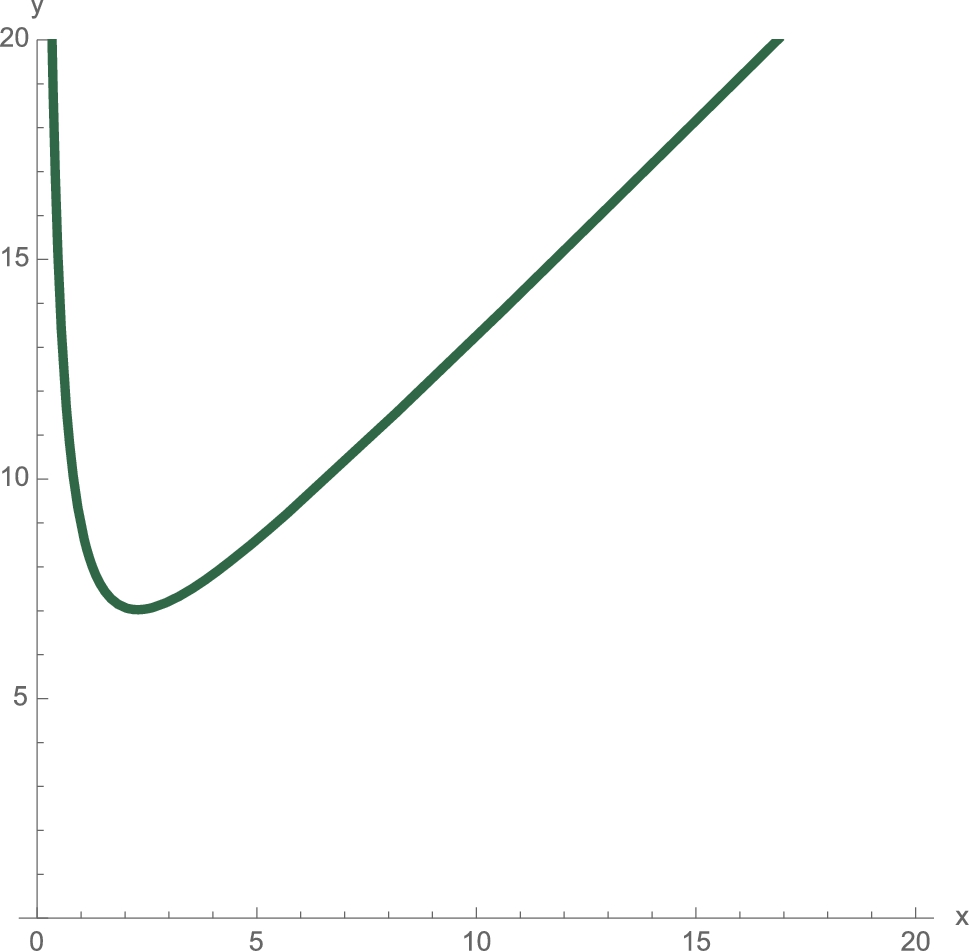
and the length of the beam, L, becomes
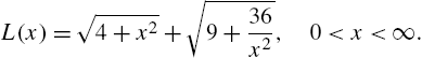
Observe that the length of the longest beam is obtained by minimizing L. (Why?)
![]()
![]()
![]()
We use two different methods to solve ![]() . Differentiating
. Differentiating
![]()
![]()
![]()
1296
![]()
![]()
![]()
![]()
and solving ![]() gives us
gives us
![]()
![]()
![]()
![]()
2.28943
![]()
![]()
![]()
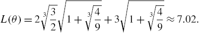
7.02348
![]()
7.02348
It follows that the length of the beam is ![]() . See Fig. 3.28.
. See Fig. 3.28.
![]()
![]()
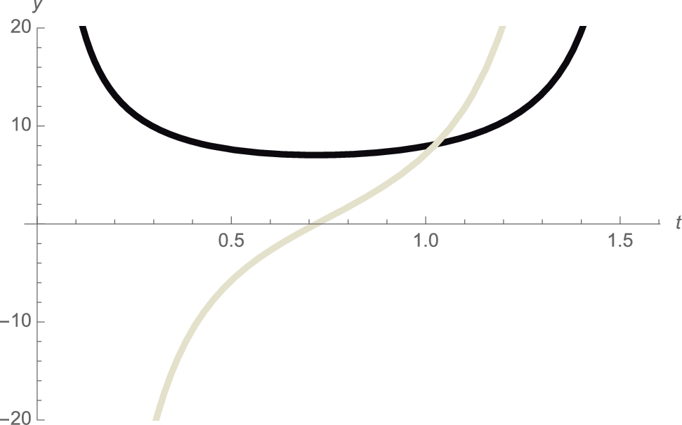
Our second approach uses right triangle trigonometry. In terms of θ, the length of the beam is given by
Differentiating gives us
To avoid typing the θ symbol, we define L as a function of t.
![]()
![]()
![]()
We now solve ![]() . First multiply through by
. First multiply through by ![]() and then by
and then by ![]() .
.
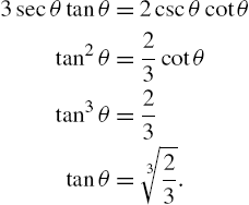
In this case, observe that we cannot compute θ exactly. However, we do not need to do so. Let ![]() be the unique solution of
be the unique solution of ![]() . See Fig. 3.29. Using the identity
. See Fig. 3.29. Using the identity ![]() , we find that
, we find that ![]() . Similarly, because
. Similarly, because ![]() and
and ![]() ,
, ![]() . Hence, the length of the beam is
. Hence, the length of the beam is
![]()
![]()
![]()
![]() □
□
In the next two examples, the constants do not have specific numerical values.
Solution
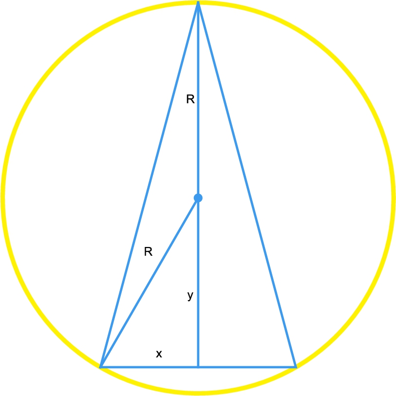
Try to avoid three-dimensional figures unless they are absolutely necessary. For this problem, a cross-section of the situation is sufficient. See Fig. 3.30, which is created with
![]()
![]()
![]()
![]()
![]()
![]()
![]()
![]()
![]()
The volume, V, of a right circular cone with radius r and height h is ![]() . Using the notation in Fig. 3.30, the volume is given by
. Using the notation in Fig. 3.30, the volume is given by
However, by the Pythagorean theorem, ![]() so
so ![]() and equation (3.4) becomes
and equation (3.4) becomes
![]()
![]()
where ![]() .
. ![]() is continuous on
is continuous on ![]() so it will have a minimum and maximum value on this interval. Moreover, the minimum and maximum values either occur at the endpoints of the interval or at the critical numbers on the interior of the interval. Differentiating equation (3.5) with respect to y gives us
so it will have a minimum and maximum value on this interval. Moreover, the minimum and maximum values either occur at the endpoints of the interval or at the critical numbers on the interior of the interval. Differentiating equation (3.5) with respect to y gives us
Remember that ![]() is a constant.
is a constant.
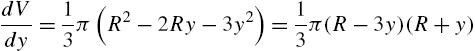
![]()
![]()
and we see that ![]() if
if ![]() or
or ![]() .
.
![]()
![]()
![]()
![]()
We ignore ![]() because −R is not in the interval
because −R is not in the interval ![]() . Note that
. Note that ![]() . The maximum volume of the cone is
. The maximum volume of the cone is

![]()
![]()
![]()
![]()
![]()
![]() □
□
Example 3.27
The Stayed-Wire Problem
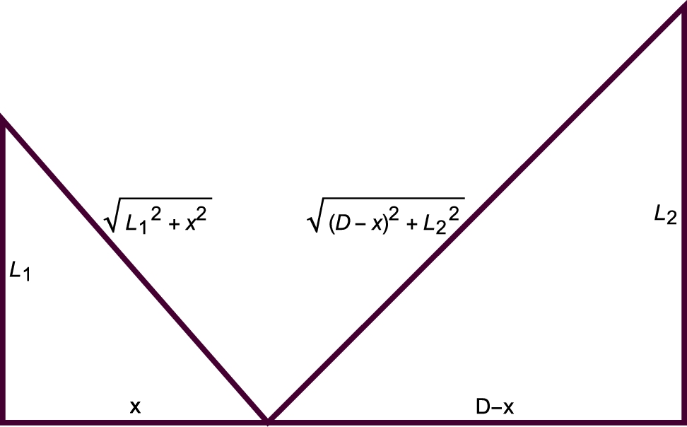
Two poles D feet apart with heights ![]() feet and
feet and ![]() feet are to be stayed by a wire as shown in Fig. 3.31. Find the minimum amount of wire required to stay the poles, as illustrated in Fig. 3.31, which is generated with
feet are to be stayed by a wire as shown in Fig. 3.31. Find the minimum amount of wire required to stay the poles, as illustrated in Fig. 3.31, which is generated with
![]()
![]()
![]()
![]()
![]()
![]()
Solution
Using the notation in Fig. 3.31, the length of the wire, L, is
In the special case that ![]() , the length of the wire to stay the beams is minimized when the wire is placed halfway between the two beams, at a distance
, the length of the wire to stay the beams is minimized when the wire is placed halfway between the two beams, at a distance ![]() from each beam. Thus, we assume that the lengths of the beams are different; we assume that
from each beam. Thus, we assume that the lengths of the beams are different; we assume that ![]() , as illustrated in Fig. 3.31. We compute
, as illustrated in Fig. 3.31. We compute ![]() and then solve
and then solve ![]() . We use PowerExpand because PowerExpand[expr] expands out all products and powers assuming the variables are real and positive. That is, with PowerExpand we obtain that
. We use PowerExpand because PowerExpand[expr] expands out all products and powers assuming the variables are real and positive. That is, with PowerExpand we obtain that ![]() rather than
rather than ![]() .
.
![]()
![]()
![]()
![]()
![]()
![]()
![]()
The result indicates that ![]() minimizes
minimizes ![]() . (Note that we ignore the other value because
. (Note that we ignore the other value because ![]() .) Moreover, the triangles formed by minimizing L are similar triangles.
.) Moreover, the triangles formed by minimizing L are similar triangles.
![]()
![]()
![]()
![]()
![]()
![]()
![]()
![]()
![]()
![]()
![]()
![]()
![]()
![]()
![]()
![]()
![]()
![]()
![]() □
□
3.2.7 Antidifferentiation
3.2.7.1 Antiderivatives
![]() is an antiderivative of
is an antiderivative of ![]() if
if ![]() . The symbols
. The symbols

mean “find all antiderivatives of ![]() .” Because all antiderivatives of a given function differ by a constant, we usually find an antiderivative,
.” Because all antiderivatives of a given function differ by a constant, we usually find an antiderivative, ![]() , of
, of ![]() and then write
and then write
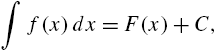
where C represents an arbitrary constant. The command
Integrate[f[x],x]
attempts to find an antiderivative, ![]() , of
, of ![]() . Instead of using Integrate, you might prefer to use the
. Instead of using Integrate, you might prefer to use the ![]() button on the Basic Math Input or Basic Math Assistant palettes to help you evaluate antiderivatives. Mathematica does not include the “+C” that we include when writing
button on the Basic Math Input or Basic Math Assistant palettes to help you evaluate antiderivatives. Mathematica does not include the “+C” that we include when writing ![]() . In the same way as D can differentiate many functions, Integrate can antidifferentiate many functions. However, antidifferentiation is a fundamentally difficult procedure so it is not difficult to find functions
. In the same way as D can differentiate many functions, Integrate can antidifferentiate many functions. However, antidifferentiation is a fundamentally difficult procedure so it is not difficult to find functions ![]() for which the command Integrate[f[x],x] returns unevaluated.
for which the command Integrate[f[x],x] returns unevaluated.
Example 3.28
Evaluate each of the following antiderivatives: (a) ![]() , (b)
, (b) ![]() , (c)
, (c) ![]() , (d)
, (d) ![]() , and (e)
, and (e) ![]() .
.
Solution
Entering
![]()
![]()
shows us that ![]() . To use the
. To use the ![]() button, first click on the button, fill in the blanks, and press Enter.
button, first click on the button, fill in the blanks, and press Enter.
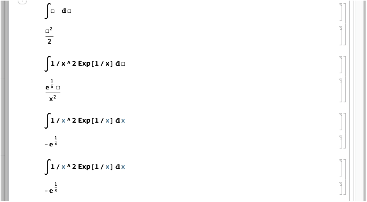
Notice that Mathematica does not automatically include the arbitrary constant, C. When computing several antiderivatives, you can use Map to apply Integrate to a list of antiderivatives. However, because Integrate is threadable,
Map[Integrate[#,x]&,list]
returns the same result as Integrate[list,x], which we illustrate to compute (b), (c), and (d).
![]()
![]()
![]()
![]()
For (e), we see that there is not a “closed form” antiderivative of ![]() and the result is given in terms of a definite integral, the sine integral function:
and the result is given in terms of a definite integral, the sine integral function:
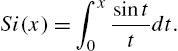
![]()
![]() □
□
u-Substitutions
Usually, the first antidifferentiation technique discussed is the method of u-substitution. Suppose that ![]() is an antiderivative of
is an antiderivative of ![]() . Given
. Given
we let ![]() so that
so that ![]() . Then,
. Then,

where ![]() is an antiderivative of
is an antiderivative of ![]() . After mastering u-substitutions, the integration by parts formula,
. After mastering u-substitutions, the integration by parts formula,
is introduced.
Example 3.29
Evaluate ![]() .
.
Solution
We use Integrate to evaluate the antiderivative.
![]()
![]()
Proceeding by hand, we let ![]() . Then,
. Then, ![]() or, equivalently,
or, equivalently, ![]()
![]()
![]()
so ![]() . We now use Integrate to evaluate
. We now use Integrate to evaluate ![]()
![]()
![]()
![]()
![]()
and then /. (ReplaceAll)/ to replace u with ![]() .
.
![]()
![]()
Observe that the result we obtained by hand is the same as the result obtained by Integrate directly. Sometimes, the results will look different and have slightly different forms. To verify that they are equivalent, subtract the two, and simplify the result. If the result is a constant, the two antiderivatives are equivalent. If not, they aren't. □
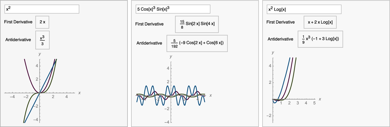
As we did with derivatives, with DynamicModule, we create a simple dynamic that lets you compute the derivative and antiderivative of basic functions and plot them on a standard viewing window, ![]() . The layout of Fig. 3.32 is primarily determined by Panel, Column, and Grid.
. The layout of Fig. 3.32 is primarily determined by Panel, Column, and Grid.
![]()
![]()
![]()
![]()
![]()
![]()
![]()
![]()
![]()
![]()
3.3 Integral Calculus
3.3.1 Area
In integral calculus courses, the definite integral is frequently motivated by investigating the area under the graph of a positive continuous function on a closed interval. Let ![]() be a nonnegative continuous function on an interval
be a nonnegative continuous function on an interval ![]() and let n be a positive integer. If we divide
and let n be a positive integer. If we divide ![]() into n subintervals of equal length and let
into n subintervals of equal length and let ![]() denote the kth subinterval, the length of each subinterval is
denote the kth subinterval, the length of each subinterval is ![]() and
and ![]() . The area bounded by the graphs of
. The area bounded by the graphs of ![]() ,
, ![]() ,
, ![]() , and the y-axis can be approximated with the sum
, and the y-axis can be approximated with the sum
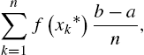
where ![]() . Typically, we take
. Typically, we take ![]() (the left endpoint of the kth subinterval),
(the left endpoint of the kth subinterval), ![]() (the right endpoint of the kth subinterval), or
(the right endpoint of the kth subinterval), or ![]() (the midpoint of the kth subinterval). For these choices of
(the midpoint of the kth subinterval). For these choices of ![]() , (3.8) becomes
, (3.8) becomes
respectively. If ![]() is increasing on
is increasing on ![]() , (3.9) is an under approximation and (3.10) is an upper approximation: (3.9) corresponds to an approximation of the area using n inscribed rectangles; (3.10) corresponds to an approximation of the area using n circumscribed rectangles. If
, (3.9) is an under approximation and (3.10) is an upper approximation: (3.9) corresponds to an approximation of the area using n inscribed rectangles; (3.10) corresponds to an approximation of the area using n circumscribed rectangles. If ![]() is decreasing on
is decreasing on ![]() , (3.10) is an under approximation and (3.9) is an upper approximation: (3.10) corresponds to an approximation of the area using n inscribed rectangles; (3.9) corresponds to an approximation of the area using n circumscribed rectangles.
, (3.10) is an under approximation and (3.9) is an upper approximation: (3.10) corresponds to an approximation of the area using n inscribed rectangles; (3.9) corresponds to an approximation of the area using n circumscribed rectangles.
In the following example, we define the functions leftsum[f[x],a,b,n], middlesum[f[x],a,b,n], and rightsum[f[x],a,b,n] to compute (3.9), (3.11), and (3.10), respectively, and leftbox[f[x],a,b,n], middlebox[f[x], a,b,n], and rightbox[f[x],a, b,n] to generate the corresponding graphs. After you have defined these functions, you can use them with functions ![]() that you define.
that you define.
Remark 3.6
To define a function of a single variable, ![]() , enter f[x_]=expression in x. To generate a basic plot of
, enter f[x_]=expression in x. To generate a basic plot of ![]() for
for ![]() , enter Plot[f[x],{x,a,b}].
, enter Plot[f[x],{x,a,b}].
Example 3.30
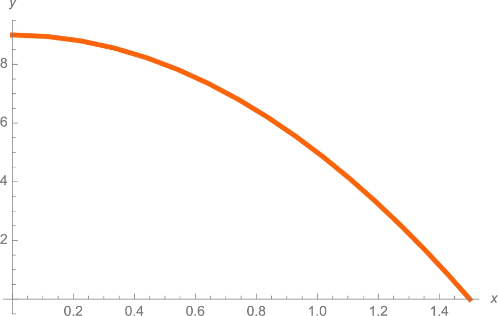
Let ![]() . Approximate the area bounded by the graph of
. Approximate the area bounded by the graph of ![]() ,
, ![]() ,
, ![]() , and the y-axis using (a) 100 inscribed and (b) 100 circumscribed rectangles. (c) What is the exact value of the area?
, and the y-axis using (a) 100 inscribed and (b) 100 circumscribed rectangles. (c) What is the exact value of the area?
Solution
We begin by defining and graphing ![]() in Fig. 3.33.
in Fig. 3.33.
![]()
![]()
![]()
![]()
The first derivative, ![]() is negative on the interval so
is negative on the interval so ![]() is decreasing on
is decreasing on ![]() . Thus, an approximation of the area using 100 inscribed rectangles is given by (3.10) while an approximation of the area using 100 circumscribed rectangles is given by (3.9). After defining leftsum, rightsum, and middlesum, these values are computed using leftsum and rightsum. The use of middlesum is illustrated as well. Approximations of the sums are obtained with N.
. Thus, an approximation of the area using 100 inscribed rectangles is given by (3.10) while an approximation of the area using 100 circumscribed rectangles is given by (3.9). After defining leftsum, rightsum, and middlesum, these values are computed using leftsum and rightsum. The use of middlesum is illustrated as well. Approximations of the sums are obtained with N.
![]()
![]()
![]()
![]()
![]()
![]()
![]()
![]()
![]()
![]()
![]()
![]()
![]()
9.06728
![]()
8.93228
![]()
9.00011
Observe that these three values appear to be close to 9. In fact, 9 is the exact value of the area of the region bounded by ![]() ,
, ![]() ,
, ![]() , and the y-axis. To help us see why this is true, we define leftbox, middlebox, and rightbox, and then use these functions to visualize the situation using
, and the y-axis. To help us see why this is true, we define leftbox, middlebox, and rightbox, and then use these functions to visualize the situation using ![]() , 16, and 32 rectangles in Fig. 3.34.
, 16, and 32 rectangles in Fig. 3.34.
It is not important that you understand the syntax of these three functions at this time. Once you have entered the code, you can use them to visualize the process for your own functions, ![]() .
.

![]()
![]()
![]()
![]()
![]()
![]()
![]()
![]()
![]()
![]()
![]()
![]()
![]()
![]()
![]()
![]()
![]()
![]()
![]()
![]()
![]()
![]()
![]()
![]()
![]()
![]()
![]()
![]()
![]()
![]()
![]()
![]()
![]()
![]()
![]()
![]()
![]()
![]()
![]()
![]()
![]()
![]()
![]()
![]()
![]()
![]()
![]()
![]()
Notice that as n increases, the under approximations increase to the value of the area while the upper approximations decrease to the value of the area. In the limit as ![]() , if the two limits are equal, we can conclude that the area is the value of the limits.
, if the two limits are equal, we can conclude that the area is the value of the limits.
These graphs help convince us that the limit of the sum as ![]() of the areas of the inscribed and circumscribed rectangles is the same. We compute the exact value of (3.9) with leftsum, evaluate and simplify the sum with Simplify, and compute the limit as
of the areas of the inscribed and circumscribed rectangles is the same. We compute the exact value of (3.9) with leftsum, evaluate and simplify the sum with Simplify, and compute the limit as ![]() with Limit. We see that the limit is 9.
with Limit. We see that the limit is 9.
![]()
![]()
![]()
![]()
![]()
9
Similar calculations are carried out for (3.10) and again we see that the limit is 9. We conclude that the exact value of the area is 9.
![]()
![]()
![]()
![]()
![]()
9
For illustrative purposes, we confirm this result with middlesum.
![]()
![]()
![]()
![]()
![]()
9
As illustrated earlier, with Manipulate, you can experiment with different functions and different n values. First, we define a set of “typical” functions.
![]()
![]()
![]()
![]()
![]()
Next, we use Manipulate to create an object that allows us to experiment with how “typical” functions react to changes in n using left, middle, and right-hand endpoint approximations for computations of Riemann sums. In the resulting Manipulate object, ![]() rectangles is the default; you can choose n-values from 0 to 100. The value of the corresponding Riemann sum is shown below the graphic. See Fig. 3.35.
rectangles is the default; you can choose n-values from 0 to 100. The value of the corresponding Riemann sum is shown below the graphic. See Fig. 3.35.
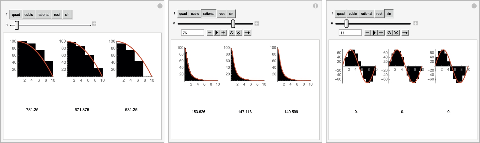
![]()
![]()
![]()
![]()
![]()
![]()
![]()
![]() □
□
3.3.2 The Definite Integral
In integral calculus courses, we formally learn that the definite integral of the function ![]() from
from ![]() to
to ![]() is
is

provided that the limit exists. In equation (3.12), ![]() is a partition of
is a partition of ![]() ,
, ![]() is the norm of P,
is the norm of P,
![]() , and
, and ![]() .
.
The Fundamental Theorem of Calculus provides the fundamental relationship between differentiation and integration.
Theorem 3.6
The Fundamental Theorem of Calculus

By the Fundamental Theorem of Calculus and the Chain Rule, it follows that
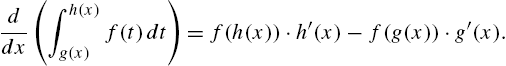
Mathematica's Integrate command can compute many definite integrals. The command
Integrate[f[x],{x,a,b}]
attempts to compute ![]() while
while
Integrate[f[x],x]
attempts to find an antiderivative of ![]() . Remember that Mathematica does not include the “+C” when computing antiderivatives. Because integration is a fundamentally difficult procedure, it is easy to create integrals for which the exact value cannot be found explicitly. In those cases, use N to obtain an approximation of its value or obtain a numerical approximation of the integral directly with
. Remember that Mathematica does not include the “+C” when computing antiderivatives. Because integration is a fundamentally difficult procedure, it is easy to create integrals for which the exact value cannot be found explicitly. In those cases, use N to obtain an approximation of its value or obtain a numerical approximation of the integral directly with
NIntegrate[f[x],{x,a,b}].
In the same way as you use the ![]() button to compute antiderivatives, you can use the
button to compute antiderivatives, you can use the ![]() button to compute definite integrals. If the result returned is unevaluated, use N to obtain a numerical approximation of the value of the integral or use NIntegrate.
button to compute definite integrals. If the result returned is unevaluated, use N to obtain a numerical approximation of the value of the integral or use NIntegrate.
Example 3.31
Evaluate (a) ![]() ; (b)
; (b) ![]() ; (c)
; (c) ![]() ; (d)
; (d) ![]() ; and (e)
; and (e) ![]() .
.
Solution
We evaluate (a)–(c) directly with Integrate.
![]()
![]()
![]()
![]()
![]()
![]()
For (d), the result returned is in terms of the error function, Erf[x], which is defined by the integral
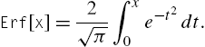
![]()
![]()
We use N to obtain an approximation of the value of the definite integral.
![]()
0.842701
(e) Recall that Mathematica does not return a real number when we compute odd roots of negative numbers so the following result would be surprising to many students in an introductory calculus course because it is complex.
![]()
![]()
Use Surd[u,n] to return the real nth root of u, ![]() , if n is odd.
, if n is odd.
![]()
![]() □
□
Improper integrals are computed using Integrate in the same way as with definite integrals.
Example 3.32
Evaluate (a) ![]() ; (b)
; (b) ![]() ; (c)
; (c) ![]() ; (d)
; (d) ![]() ; (e)
; (e) ![]() ; and (f)
; and (f) ![]() .
.
Solution
(a) This is an improper integral because the integrand is discontinuous on the interval ![]() but we see that the improper integral converges to −4.
but we see that the improper integral converges to −4.
![]()
−4
(b) This is an improper integral because the interval of integration is infinite but we see that the improper integral converges to 2.
![]()
2
(c) This is an improper integral because the integrand is discontinuous on the interval of integration and because the interval of integration is infinite but we see that the improper integral converges to ![]() .
.
![]()
![]()
(d) As with (c), this is an improper integral because the integrand is discontinuous on the interval of integration and because the interval of integration is infinite but we see that the improper integral diverges to ∞.

(e) Recall that Mathematica does not return a real number when we compute odd roots of negative numbers so the following result would be surprising to many students in an introductory calculus course because it contains imaginary numbers.
![]()
![]()
Therefore, we use Surd to obtain the real-valued third root of ![]() .
.
![]()
6
(f) In this case, Mathematica warns us that the improper integral diverges.
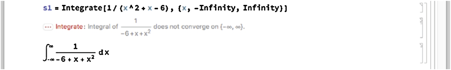
To help us understand why the improper integral diverges, we note that ![]() and
and

![]()
![]()
Hence the integral is improper because the interval of integration is infinite and because the integrand is discontinuous on the interval of integration so
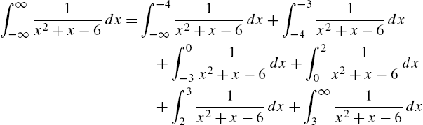
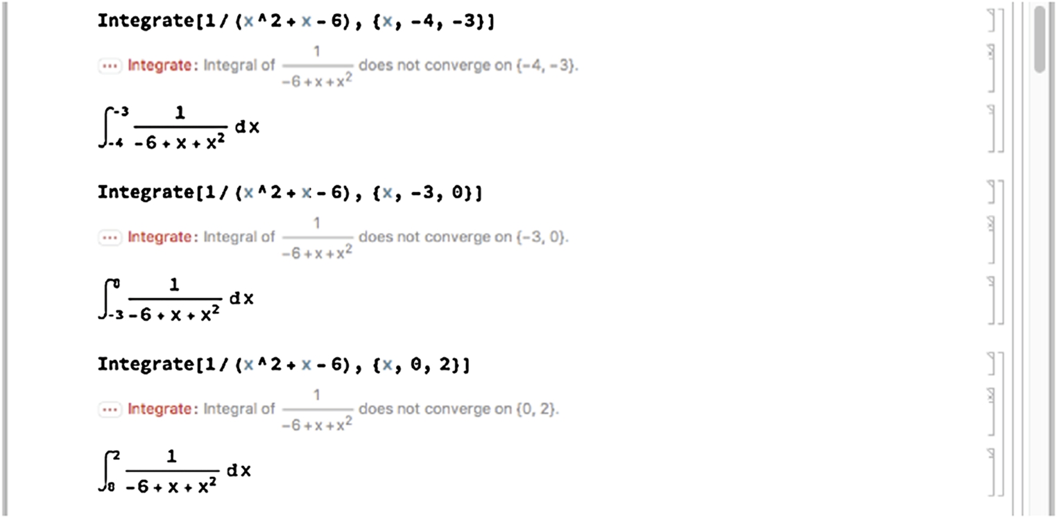
Evaluating each of these integrals,
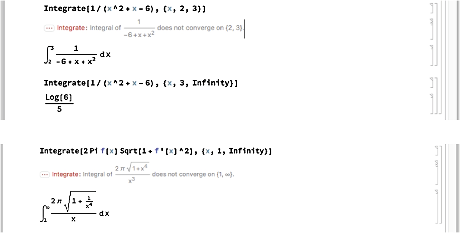
we conclude that the improper integral diverges because at least one of the improper integrals in (3.13) diverges. □
In many cases, Mathematica can help illustrate the steps carried out when computing integrals using standard methods of integration like u-substitutions and integration by parts.
Example 3.33
Evaluate (a) ![]() and (b)
and (b) ![]() .
.
Solution
(a) We let ![]() . Then,
. Then, ![]() so
so
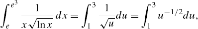
which we evaluate with Integrate.
The new lower limit of integration is 1 because if ![]() ,
, ![]() . The new upper limit of integration is 3 because if
. The new upper limit of integration is 3 because if ![]() ,
, ![]() .
.
![]()
![]()
To evaluate (b), we let ![]() and
and ![]() .
.
![]()
![]()
![]()
![]()
1
![]()
The results mean that
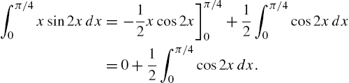
The resulting indefinite integral is evaluated with Integrate.
![]()
![]()
Alternatively, we can illustrate the integration by parts calculation, ![]() .
.
![]()
![]()
We use Integrate to evaluate the definite integral.
![]()
![]() □
□
3.3.3 Approximating Definite Integrals
Because integration is a fundamentally difficult procedure to produce exact answers or results, Mathematica is unable to compute a “closed form” of the value of many definite integrals. In these cases, numerical integration can be used to obtain an approximation of the definite integral using N together with Integrate or NIntegrate:
NIntegrate[f[x],{x,a,b}]
attempts to approximate ![]() .
.
Example 3.34
Evaluate ![]() .
.
Solution
In this case, Mathematica is unable to evaluate the integral with Integrate.
We use the ![]() button to complete the Integrate command.
button to complete the Integrate command.
![]()
![]()
An approximation is obtained with N.
![]()
0.701566
Instead of using Integrate followed by N, you can use NIntegrate to numerically evaluate the integral.
![]()
0.701566
returns the same result as that obtained using Integrate followed by N. □
In some cases, you may wish to investigate particular numerical methods that can be used to approximate integrals. To implement numerical methods like Simpson's rule or the trapezoidal rule, redefine the function leftsum (middlesum or rightsum) discussed previously to perform the calculation for the desired method.
3.3.4 Area
Suppose that ![]() and
and ![]() are continuous on
are continuous on ![]() and that
and that ![]() for
for ![]() . The area of the region bounded by the graphs of
. The area of the region bounded by the graphs of ![]() ,
, ![]() ,
, ![]() , and
, and ![]() is
is
Sometimes determining the “greater” function and the “lower” function can be difficult. Equation (3.14) in its more general form tells us that the region bounded by the graphs of ![]() ,
, ![]() ,
, ![]() , and
, and ![]() is
is

Example 3.35
Find the area between the graphs of ![]() and
and ![]() on the interval
on the interval ![]() .
.
Solution
We graph ![]() and
and ![]() on the interval
on the interval ![]() in Fig. 3.36 with Plot. The graph of
in Fig. 3.36 with Plot. The graph of ![]() is dashed. Observe that including the option Filling->{1->{2}} fills the region between the two plots.
is dashed. Observe that including the option Filling->{1->{2}} fills the region between the two plots.
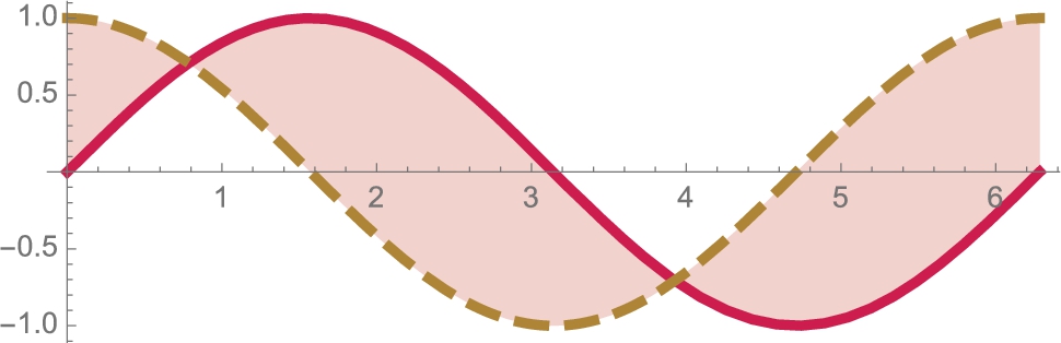
 and
and  on the interval [0,2π] (University of Wisconsin colors).
![]()
![]()
![]()
![]()
To find the upper and lower limits of integration, we must solve the equation ![]() for x. Observe that Mathematica returns all solutions to the equation that it can find. The results show us that there are infinitely many solutions to the equation.
for x. Observe that Mathematica returns all solutions to the equation that it can find. The results show us that there are infinitely many solutions to the equation.
![]()
![]()
![]()
For us the solutions of interest are valid for ![]() , which are
, which are ![]() and
and ![]() . We check that these are valid solutions of
. We check that these are valid solutions of ![]() with ==; in each case the returned result is True.
with ==; in each case the returned result is True.
![]()
![]()
True
True
Hence, the area of the region between the graphs is given by

Notice that if we take advantage of symmetry we can simplify (3.16) to
We evaluate (3.17) with Integrate to see that the area of the region between the two graphs is ![]() .
.
![]()
![]() □
□
In cases when we cannot calculate the points of intersection of two graphs exactly, we can frequently use FindRoot to approximate the points of intersection.
Example 3.36
Solution
After defining p and q, we graph them on the interval ![]() in Fig. 3.37 to obtain an initial guess of the intersection points of the two graphs.
in Fig. 3.37 to obtain an initial guess of the intersection points of the two graphs.
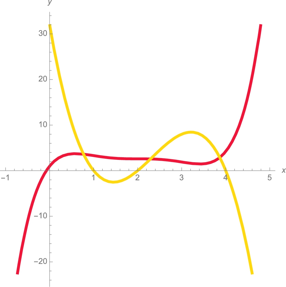
![]()
![]()
![]()
![]()
![]()
![]()
![]()
The x-coordinates of the three intersection points are the solutions of the equation ![]() . Although Mathematica can solve this equation exactly, approximate solutions are more useful for the problem and obtained with NSolve.
. Although Mathematica can solve this equation exactly, approximate solutions are more useful for the problem and obtained with NSolve.
![]()
![]()
The numbers are extracted from the list with Part ([[...]]). For example, 0.772058 is the second part of the first part of intpts. Counting from left to right, 2.29182 is the second part of the fourth part of intpts.
![]()
![]()
![]()
0.772058
2.29182
3.86513
Using the roots to the equation ![]() and the graph we see that
and the graph we see that ![]() for
for ![]() and
and ![]() for
for ![]() . Hence, an approximation of the area bounded by
. Hence, an approximation of the area bounded by ![]() and
and ![]() is given by the sum
is given by the sum
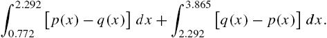
These two integrals are computed with Integrate and NIntegrate. As expected, the two values are the same.
![]()
12.1951
![]()
12.1951
We conclude that the area is approximately 12.195 units2. □
Parametric Equations
If the curve, C, defined parametrically by ![]() ,
, ![]() ,
, ![]() is a nonnegative continuous function of x and
is a nonnegative continuous function of x and ![]() the area under the graph of C and above the x-axis is
the area under the graph of C and above the x-axis is

Graphically, y is a function of x, ![]() , if the graph of
, if the graph of ![]() passes the vertical line test.
passes the vertical line test.
Example 3.37
The Astroid
Find the area enclosed by the astroid ![]() ,
, ![]() ,
, ![]() .
.
Solution
We begin by defining x and y and then graphing the astroid with ParametricPlot in Fig. 3.38.
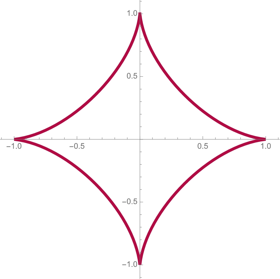
 ,
,  , 0 ⩽ t ⩽ 2π (Harvard University colors).
![]()
![]()
![]()
![]()
Observe that ![]() and
and ![]() and the graph of the astroid in the first quadrant is given by
and the graph of the astroid in the first quadrant is given by ![]() ,
, ![]() ,
, ![]() . Hence, the area of the astroid in the first quadrant is given by
. Hence, the area of the astroid in the first quadrant is given by
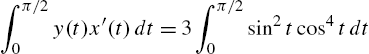
and the total area is given by

which is computed with Integrate and then approximated with N.
![]()
![]()
![]()
1.1781 □
Polar Coordinates
For problems involving “circular symmetry” it is often easier to work in polar coordinates. The relationship between ![]() in rectangular coordinates and
in rectangular coordinates and ![]() in polar coordinates is given by
in polar coordinates is given by
and
If ![]() is continuous and nonnegative for
is continuous and nonnegative for ![]() , then the area A of the region enclosed by the graphs of
, then the area A of the region enclosed by the graphs of ![]() ,
, ![]() , and
, and ![]() is
is
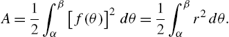
Example 3.38
Lemniscate of Bernoulli
Solution
This problem is much easier solved in polar coordinates so we first convert the equation from rectangular to polar coordinates with ReplaceAll (/.) and then solve for r with Solve.
![]()
![]()
![]()
![]()
![]()
These results indicate that an equation of the lemniscate in polar coordinates is ![]() . The graph of the lemniscate is then generated in Fig. 3.39 (top figure) using PolarPlot. The portion of the lemniscate in quadrant one is obtained by graphing
. The graph of the lemniscate is then generated in Fig. 3.39 (top figure) using PolarPlot. The portion of the lemniscate in quadrant one is obtained by graphing ![]() ,
, ![]() .
.
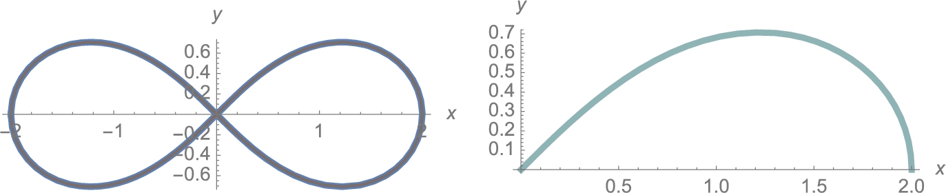
![]()
![]()
![]()
![]()
![]()
![]()
![]()
Then, taking advantage of symmetry, the area of the lemniscate is given by

which we calculate with Integrate.
![]()
![]() □
□
3.3.5 Arc Length
Let ![]() be a function for which
be a function for which ![]() is continuous on an interval
is continuous on an interval ![]() . Then the arc length of the graph of
. Then the arc length of the graph of ![]() from
from ![]() to
to ![]() is given by
is given by
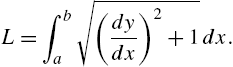
The resulting definite integrals used for determining arc length are usually difficult to compute because they involve a radical. In these situations, Mathematica is helpful with approximating solutions to these types of problems.
Example 3.39
Find the length of the graph of ![]() from (a)
from (a) ![]() to
to ![]() and from (b)
and from (b) ![]() to
to ![]() .
.
Solution
With no restrictions on the value of x, ![]() . Generally, Mathematica does not automatically algebraically simplify
. Generally, Mathematica does not automatically algebraically simplify ![]() because Mathematica does not know if x is positive or negative.
because Mathematica does not know if x is positive or negative.
![]()
![]()
![]()
![]()
![]()
In fact, for (b), x is negative so  . Mathematica simplifies
  and correctly evaluates the arc length integral (3.18) for (a).
![]()
![]()
For (b), we compute the arc length integral (3.18).
![]()
![]()
As we expect, both values are the same. □
Parametric Equations
If the smooth curve, C, defined parametrically by ![]() ,
, ![]() ,
, ![]() is traversed exactly once as t increases from
is traversed exactly once as t increases from ![]() to
to ![]() , the arc length of C is given by
, the arc length of C is given by

C is smooth if both ![]() and
and ![]() are continuous on
are continuous on ![]() and not simultaneously zero for
and not simultaneously zero for ![]() .
.
Example 3.40
Find the length of the graph of ![]() ,
, ![]() ,
, ![]() .
.
Solution
For illustrative purposes, we graph ![]() ,
, ![]() for
for ![]() and
and ![]() (thickened) in Fig. 3.40.
(thickened) in Fig. 3.40.
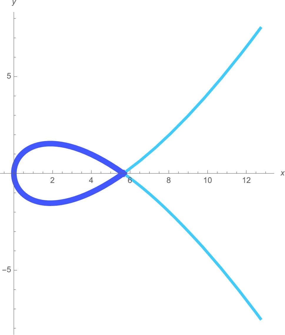
 ,
,  (Pennsylvania State University colors).
![]()
![]()
![]()
![]()
![]()
![]()
Mathematica is able to compute the exact value of the arc length (3.19) although the result is quite complicated. For length considerations, the result of entering the i1 command are not displayed here.
![]()
![]()
![]()
![]()
A more meaningful approximation is obtained with N or using NIntegrate.
![]()
13.7099
![]()
13.7099
We conclude that the arc length is approximately 13.71.
Observe that Mathematica 11 cannot evaluate the definite integral directly. However, if we first compute an anti-derivative with integrate in i2,
![]()
![]()
![]()
![]()
and then apply the Fundamental Theorem of Calculus by subtracting the value of i2 if ![]() from the value of i2 if
from the value of i2 if ![]() ,
,
![]()
![]()
![]()
![]()
![]()
![]()
0
![]()
![]()
![]()
![]()
![]()
![]()
13.7099
we obtain the same result. □
Polar Coordinates
If the smooth polar curve C given by ![]() ,
, ![]() is traversed exactly once as θ increases from α to β, the arc length of C is given by
is traversed exactly once as θ increases from α to β, the arc length of C is given by
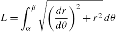
Example 3.41
Find the length of the graph of ![]() ,
, ![]() .
.
Solution
We begin by defining r and then graphing r with PolarPlot in Fig. 3.41.
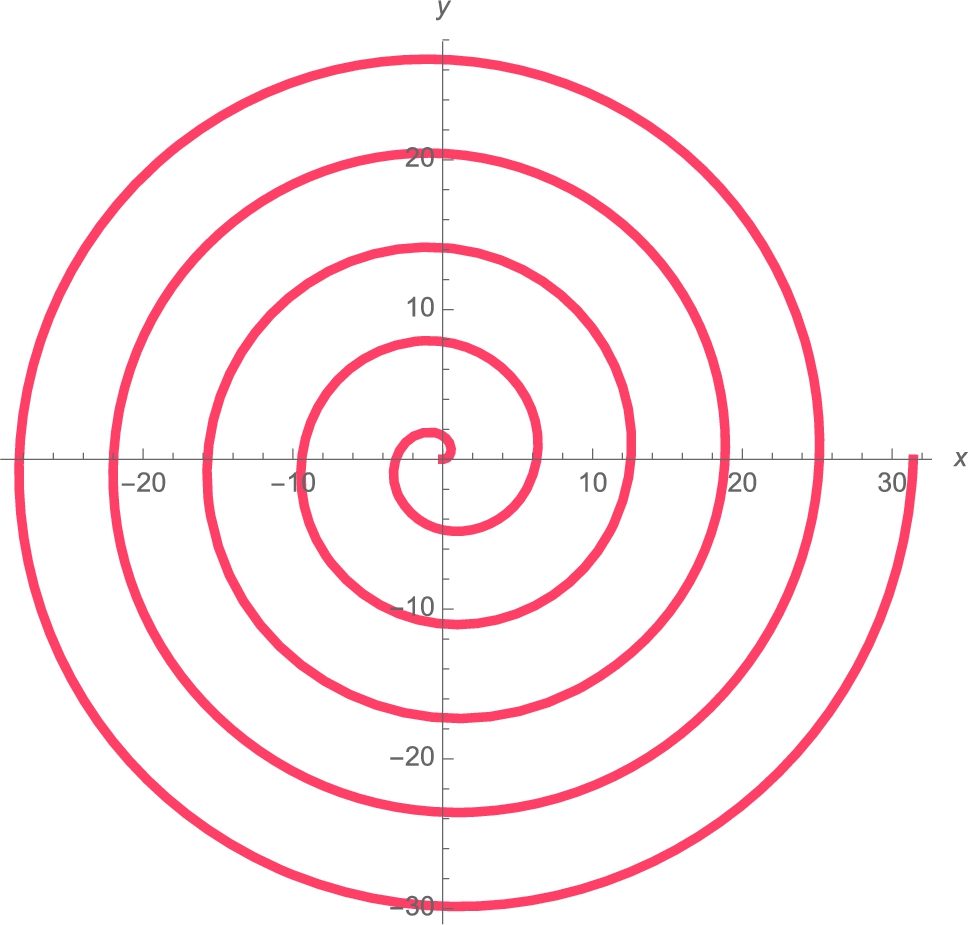
![]()
![]()
![]()
![]()
Using (3.20), the length of the graph of r is given by ![]() . The exact value is computed with Integrate
. The exact value is computed with Integrate
![]()
![]()
and then approximated with N.
![]()
495.801
We conclude that the length of the graph is approximately 495.8 units. □
3.3.6 Solids of Revolution
Volume
Let ![]() be a nonnegative continuous function on
be a nonnegative continuous function on ![]() . The volume of the solid of revolution obtained by revolving the region bounded by the graphs of
. The volume of the solid of revolution obtained by revolving the region bounded by the graphs of ![]() ,
, ![]() ,
, ![]() , and the x-axis about the x-axis is given by
, and the x-axis about the x-axis is given by

If ![]() , the volume of the solid of revolution obtained by revolving the region bounded by the graphs of
, the volume of the solid of revolution obtained by revolving the region bounded by the graphs of ![]() ,
, ![]() ,
, ![]() , and the x-axis about the y-axis is given by
, and the x-axis about the y-axis is given by

Example 3.42
Let ![]() . Find the volume of the solid obtained by revolving the region bounded by the graphs of
. Find the volume of the solid obtained by revolving the region bounded by the graphs of ![]() ,
, ![]() ,
, ![]() , and the x-axis about (a) the x-axis; and (b) the y-axis.
, and the x-axis about (a) the x-axis; and (b) the y-axis.
Solution
After defining g, we graph g on the interval ![]() in Fig. 3.42 (a).
in Fig. 3.42 (a).
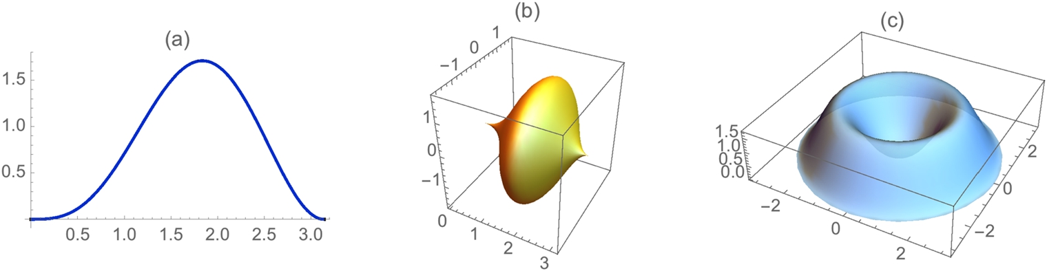
![]()
![]()
![]()
![]()
The volume of the solid obtained by revolving the region about the x-axis is given by equation (3.21) while the volume of the solid obtained by revolving the region about the y-axis is given by equation (3.22). These integrals are computed with Integrate and named xvol and yvol, respectively. We use N to approximate each volume.
![]()
![]()
![]()
9.86295
![]()
![]()
![]()
27.5349
We can use ParametricPlot3D to visualize the resulting solids by parametrically graphing the equations given by
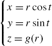
for r between 0 and π and t between −π and π to visualize the graph of the solid obtained by revolving the region about the y-axis and by parametrically graphing the equations given by

for r between 0 and π and t between −π and π to visualize the graph of the solid obtained by revolving the region about the x-axis. (See Figs. 3.42 (b) and 3.42 (c).) In this case, we identify the z-axis as the y-axis. Notice that we are simply using polar coordinates for the x and y-coordinates, and the height above the x, y-plane is given by ![]() because r is replacing x in the new coordinate system.
because r is replacing x in the new coordinate system.
![]()
![]()
![]()
![]()
![]()
![]()
![]()
![]()
![]()
p1, p2, and p3 are shown together side-by-side in Fig. 3.42 using Show together with GraphicsRow.
![]() □
□
We now demonstrate a volume problem that requires the method of disks.
Example 3.43
Let ![]() . Approximate the volume of the solid obtained by revolving the region bounded by the graphs of
. Approximate the volume of the solid obtained by revolving the region bounded by the graphs of ![]() ,
, ![]() ,
, ![]() , and the x-axis about the x-axis.
, and the x-axis about the x-axis.
Solution
Proceeding as in the previous example, we first define and graph f on the interval ![]() in Fig. 3.43 (a).
in Fig. 3.43 (a).
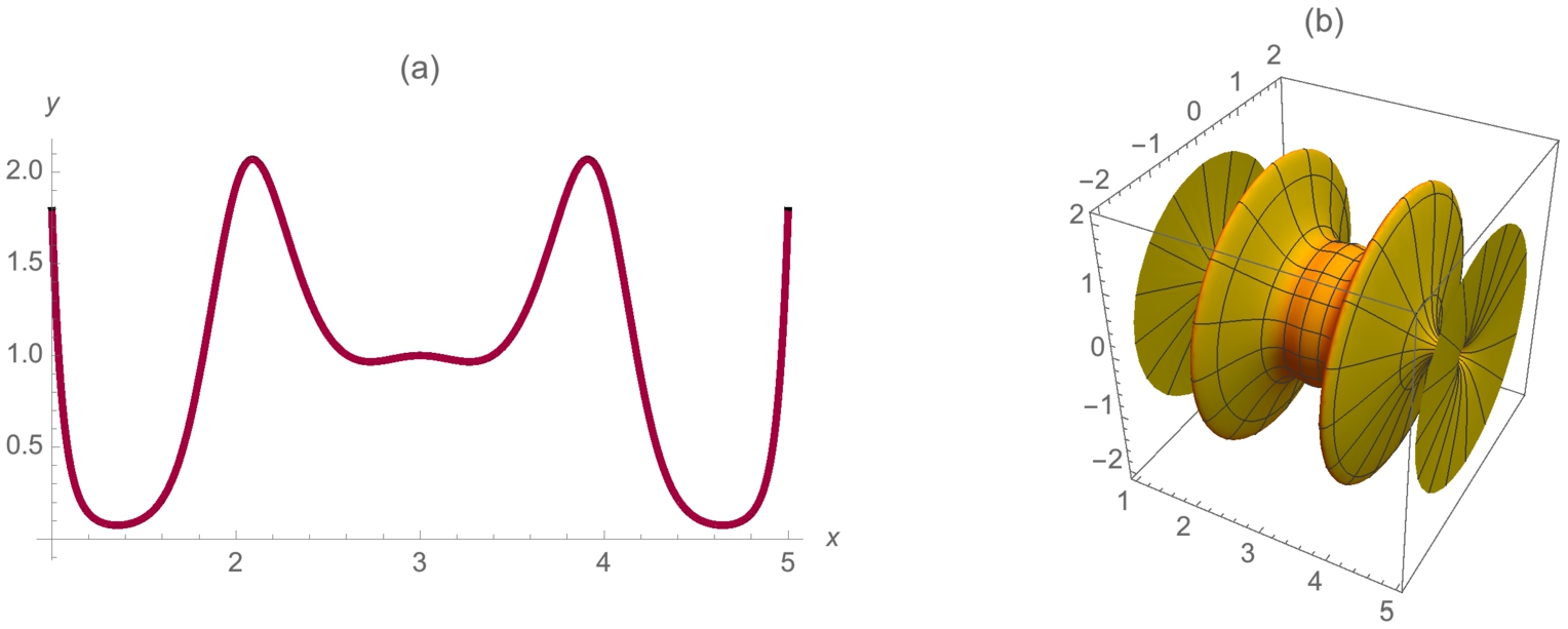
![]()
![]()
![]()
![]()
In this case, an approximation is desired so we use NIntegrate to approximate the integral ![]() .
.
![]()
16.0762
In the same manner as before, ParametricPlot3D can be used to visualize the resulting solid by graphing the set of equations given parametrically by
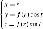
for r between 1 and 5 and t between 0 and 2π. In this case, polar coordinates are used in the y, z-plane with the distance from the x-axis given by ![]() . Because r replaces x in the new coordinate system,
. Because r replaces x in the new coordinate system, ![]() becomes
becomes ![]() in these equations. See Fig. 3.43 (b).
in these equations. See Fig. 3.43 (b).
![]()
![]()
![]()
![]() □
□
When revolving a curve about the y-axis, you can use RevolutionPlot3D rather than the parametrization given previously.
Example 3.44
Let ![]() for
for ![]() . (a) Find the minimum and maximum values of
. (a) Find the minimum and maximum values of ![]() on
on ![]() . Let R be the region bounded by
. Let R be the region bounded by ![]() ,
, ![]() ,
, ![]() , and the y-axis. (b) Find the volume of the solid obtained by revolving R about the y-axis. (c) Find the volume of the solid obtained by revolving R about the x-axis.
, and the y-axis. (b) Find the volume of the solid obtained by revolving R about the y-axis. (c) Find the volume of the solid obtained by revolving R about the x-axis.
Solution
(a) Although Maximize and Minimize cannot find the exact maximum and minimum values, using N or NMaximize and NMinimize give accurate approximations.
![]()
![]()
![]()
![]()
![]()
![]()
![]()
![]()
![]()
![]()
![]()
![]()
![]()
![]()
![]()
![]()
![]()
We double check these results by graphing ![]() and
and ![]() in Fig. 3.44 and then using FindRoot to approximate the critical numbers.
in Fig. 3.44 and then using FindRoot to approximate the critical numbers.
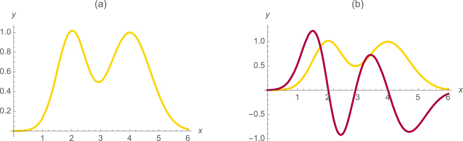
![]()
![]()
![]()
![]()
![]()
![]()
![]()
![]()
![]()
(b) Mathematica finds the exact volume of the solids although the results are expressed in terms of the Error function, Erf.
![]()
![]()
![]()
30.0673
![]()
![]()
![]()
7.1682
To visualize the solid revolved about the y-axis, we use RevolutionPlot3D in p1. We generate the curve in p2, a set of axes, and a representative “slice” of the curve. See Fig. 3.45 (a). After, we show the solid together with a representative shell. See Fig. 3.45 (b).
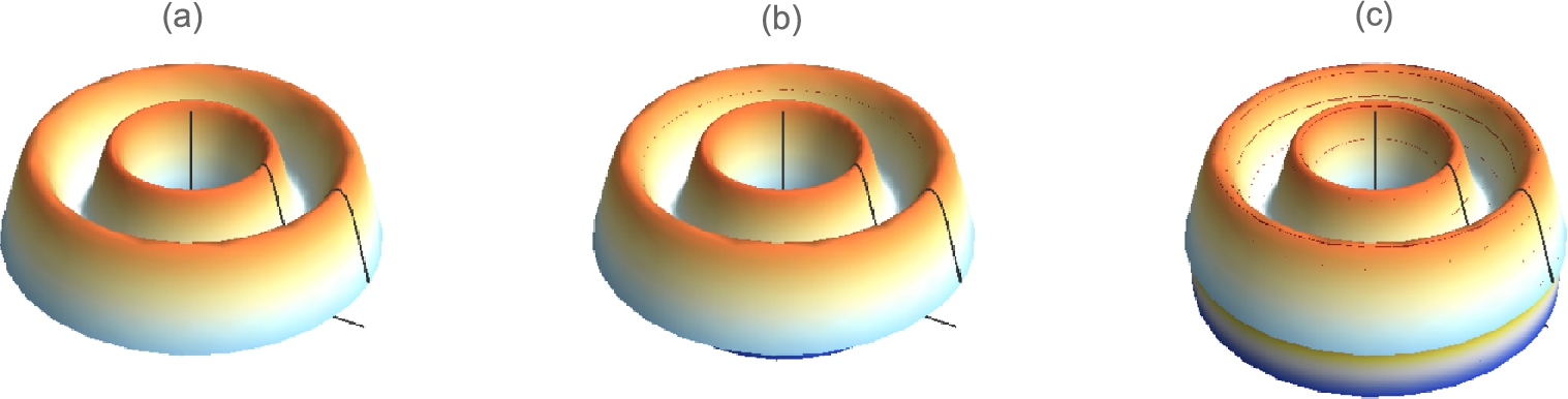
![]()
![]()
![]()
![]()
![]()
![]()
![]()
![]()
![]()
![]()
![]()
![]()
![]()
![]()
![]()
![]()
![]()
![]()
![]()
![]()
![]()
![]()
Finally, we show the solid together with several shells in Fig. 3.45 (c).
![]()
![]()
![]()
![]()
![]()
![]()
![]()
![]()
![]()
You can use Animate to animate the process as illustrated in Fig. 3.46.

![]()
![]()
![]()
![]()
![]()
![]()
For revolving ![]() about the x-axis, we proceed in much the same way. First, we plot
about the x-axis, we proceed in much the same way. First, we plot ![]() with a set of axes in three-space.
with a set of axes in three-space.
![]()
![]()
![]()
![]()
![]()
![]()
![]()
![]()
![]()
![]()
![]()
![]()
(c) Next, we generate a basic plot of the solid in p4 and then a set of disks inside the solid in t3d.
![]()
![]()
![]()
![]()
![]()
![]()
![]()
![]()
![]()
![]()
![]()
![]()
![]()
![]()
![]()
![]()
![]()
![]()
Two variations of the solid are plotted in p5 and p6. In each case, we use MeshFunctions to have the contour lines (mesh) correspond to ![]() values rather than the rectangular default mesh. In p6 the solid is made transparent with the Opacity option.
values rather than the rectangular default mesh. In p6 the solid is made transparent with the Opacity option.
![]()
![]()
![]()
![]()
![]()
![]()
![]()
![]()
![]()
![]()
Several combinations of the images are shown in Figs. 3.47 and 3.48.
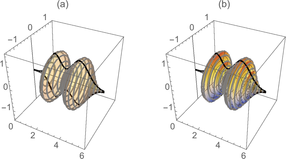
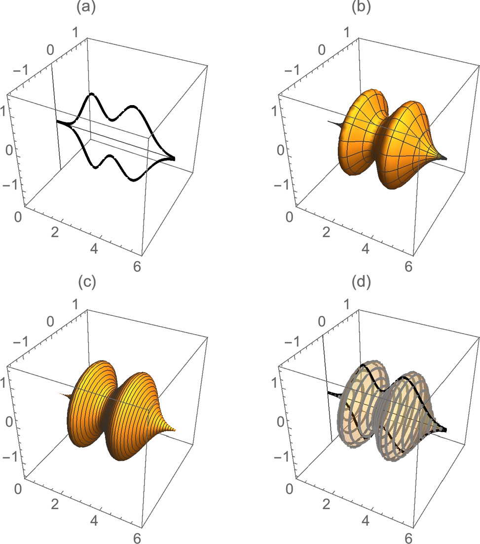
![]()
![]()
![]() □
□
To help identify regions, RegionPlot[constraints,{x,a,b},{y,a,b}] attempts to shade the region in the rectangle ![]() that satisfies the constraints in constraints.
that satisfies the constraints in constraints.
Example 3.45
Let ![]() ,
, ![]() , and R the region bounded by the graphs of
, and R the region bounded by the graphs of ![]() and
and ![]() . Find the volume of the solid obtained by revolving R about (a) the x-axis and (b) the y-axis.
. Find the volume of the solid obtained by revolving R about (a) the x-axis and (b) the y-axis.
Solution
We illustrate the use of RegionPlot to help us see R. See Fig. 3.49

 . (c) The two plots displayed together.
![]()
![]()
![]()
![]()
![]()
![]()
![]()
![]()
We plot the solids with ParametricPlot3D and contour lines along the function values using the MeshFunctions option in Fig. 3.50.
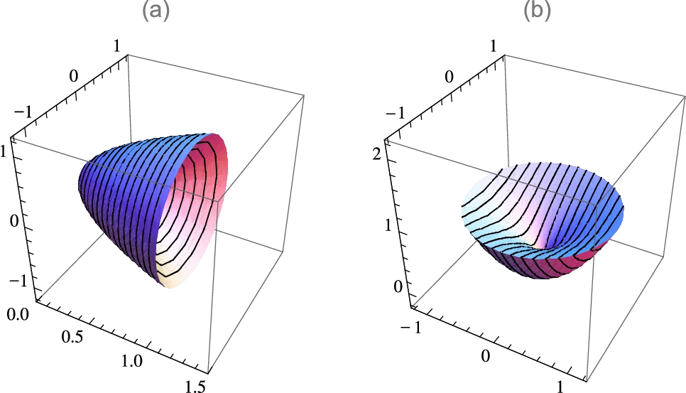
![]()
![]()
![]()
![]()
![]()
![]()
![]()
![]()
![]()
![]()
![]()
The volume of each solid is then found with Integrate and approximated with N.
![]()
![]()
![]()
0.942478
![]()
![]()
![]()
0.471239 □
Surface Area
Let ![]() be a nonnegative function for which
be a nonnegative function for which ![]() is continuous on an interval
is continuous on an interval ![]() . Then the surface area of the solid of revolution obtained by revolving the region bounded by the graphs of
. Then the surface area of the solid of revolution obtained by revolving the region bounded by the graphs of ![]() ,
, ![]() ,
, ![]() , and the x-axis about the x-axis is given by
, and the x-axis about the x-axis is given by
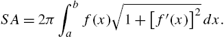
Example 3.46
Gabriel's Horn
Gabriel's horn is the solid of revolution obtained by revolving the area of the region bounded by ![]() and the x-axis for
and the x-axis for ![]() about the x-axis. Show that the surface area of Gabriel's horn is infinite but that its volume is finite.
about the x-axis. Show that the surface area of Gabriel's horn is infinite but that its volume is finite.
Solution
After defining ![]() , we use ParametricPlot3D to visualize a portion of Gabriel's horn in Fig. 3.51.
, we use ParametricPlot3D to visualize a portion of Gabriel's horn in Fig. 3.51.

![]()
![]()
![]()
Using equation (3.23), the surface area of Gabriel's horn is given by the improper integral
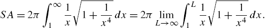
![]()
![]()
![]()

![]()
![]()
![]()
![]()
∞
On the other hand, using equation (3.21) the volume of Gabriel's horn is given by the improper integral

which converges to π.
![]()
![]()
![]()
π
![]()
π □
3.4 Infinite Sequences and Series
3.4.1 Introduction to Sequences
Sequences and series are usually discussed in the third quarter or second semester of introductory calculus courses. Most students find that it is one of the most difficult topics covered in calculus. A sequence is a function with domain consisting of the positive integers. The terms of the sequence ![]() are
are ![]() ,
, ![]() ,
, ![]() , …. The nth term is
, …. The nth term is ![]() ; the
; the ![]() st term is
st term is ![]() . If
. If ![]() , we say that
, we say that ![]() converges to L. If
converges to L. If ![]() does not converge,
does not converge, ![]() diverges. We can sometimes prove that a sequence converges by applying the following theorem.
diverges. We can sometimes prove that a sequence converges by applying the following theorem.
Theorem 3.7
Every bounded monotonic sequence converges.
A sequence ![]() is monotonic if
is monotonic if ![]() is increasing (
is increasing (![]() for all n) or decreasing (
for all n) or decreasing (![]() for all n).
for all n).
In particular, Theorem 3.7 gives us the following special cases.
1. If ![]() has positive terms and is eventually decreasing,
has positive terms and is eventually decreasing, ![]() converges.
converges.
2. If ![]() has negative terms and is eventually increasing
has negative terms and is eventually increasing ![]() converges.
converges.
After you have defined a sequence, use Table to compute the first few terms of the sequence.
1. Table[a[n],{n,1,m}] returns the list ![]() .
.
2. Table[a[n],{n,k,m}] returns ![]() .
.
The command ListPlot[listofpoints] plots the list of points listofpoints while ListLinePlot[listofpoints] plots the list of points listofpoints and connects consecutive points with line segments.
Example 3.47
If ![]() , show that
, show that ![]() .
.
Solution
We remark that the symbol n! in the denominator of ![]() represents the factorial sequence:
represents the factorial sequence:
We begin by defining ![]() and then computing the first few terms of the sequence with Table.
and then computing the first few terms of the sequence with Table.
![]()
![]()
![]()
![]()
![]()
![]()
![]()
![]()
The first few terms increase in magnitude. In fact, this is further confirmed by graphing the first few terms of the sequence with ListPlot in Fig. 3.52 (a). Based on the graph and the values of the first few terms we might incorrectly conclude that the sequence diverges.
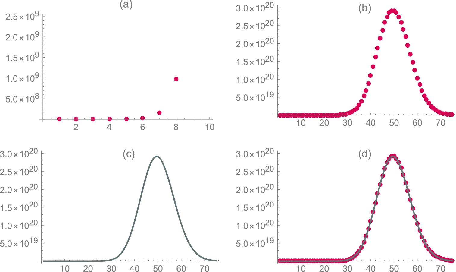
![]()
![]()
However, notice that ![]() . Because
. Because ![]() for
for ![]() , we conclude that the sequence is decreasing for
, we conclude that the sequence is decreasing for ![]() . Because it has positive terms, it is bounded below by 0 so the sequence converges by Theorem 3.7. Let
. Because it has positive terms, it is bounded below by 0 so the sequence converges by Theorem 3.7. Let ![]() . Then,
. Then,
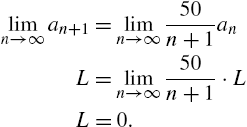
When we graph a larger number of terms, it is clear that the limit is 0. (See Fig. 3.52 (b).) It is a good exercise to show that for any real value of x, ![]() .
.
![]()
![]()
![]()
![]()
![]()
![]()
![]()
![]() □
□
Example 3.48
The Rational Numbers and the Calkin–Wilf Sequence
A set S is countably infinite if there is a one-to-one correspondence between the elements of S and the natural numbers. In other words, S is countably infinite if it can be written as a sequence.
Students in introductory set theory classes often learn that the set of rational numbers, ![]() is countably infinite using Cantor's Diagnalization Process.
is countably infinite using Cantor's Diagnalization Process.
In 2000, Neil Calkin and Herbert Wilf published a paper introducing the Calkin–Wilf sequence. The Calkin–Wilf sequence is a recursively defined sequence that gives a one-to-one correspondence between the natural numbers and the positive rational numbers. Stating a specific sequence that yields the positive rational numbers proving the countability of the rationals provides an interesting contrast to the traditional method of using Cantor's Diagnalization Process.
The Calkin–Wilf sequence is defined by
where ![]() represents the integer part of
represents the integer part of ![]() . The Mathematica command IntegerPart[x] returns the integer part of x. When defining q, observe that we use the form q[i_]:=q[i]= so that Mathematica “remembers” the computed values of
. The Mathematica command IntegerPart[x] returns the integer part of x. When defining q, observe that we use the form q[i_]:=q[i]= so that Mathematica “remembers” the computed values of ![]() . Thus, to compute
. Thus, to compute ![]() , Mathematica need only have computed
, Mathematica need only have computed ![]() rather than re-computing the previous
rather than re-computing the previous ![]()
![]() values. Compute and plot the first n terms of the Calkin–Wilf sequence with
values. Compute and plot the first n terms of the Calkin–Wilf sequence with ![]() and
and ![]() .
.
Solution
![]()
![]()
![]()
In q1 we compute the first 50 terms of the Calkin–Wilf sequence while in q2 we compute the first 500 terms of the Calkin–Wilf but do not display the result.
![]()
![]()
![]()
We then graph both sets of points with ListPlot and show the results in Fig. 3.53.
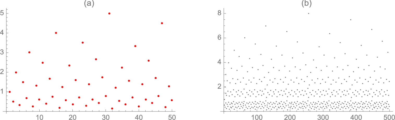
![]()
![]()
![]()
![]()
![]() □
□
You can use Mathematica to define quite complex sequences. In the following example, we define a sequence that depends on four other sequences. Observe that when defining the terms, we consistently use the form a[n_]:=a[n]=... so that Mathematica “remembers” sequence values computed and need not recompute them to compute subsequent terms.
Example 3.49
The Gauss–Legendre Algorithm
One algorithm to approximate π is the Gauss–Legendre algorithm. Although it is memory intensive, 25 iterations approximate π to around 45 million digits. After defining ![]() ,
, ![]() ,
, ![]() , and
, and ![]() , π is approximated with
, π is approximated with ![]() . Approximate π to 100 decimal places.
. Approximate π to 100 decimal places.
Solution
![]()
![]()
![]()
![]()
![]()
![]()
![]()
![]()
![]()
π is then approximated with
![]()
To increase the accuracy of your approximation, increase 10000 and 100 to your desired values. However, even on relatively fast machines, if you replace all these numbers with a number such as 1000000, the computation time will increase considerably.
For illustrate purposes, we approximate π with ![]() . Observe that the result is accurate to at least 100 decimal places.
. Observe that the result is accurate to at least 100 decimal places.
![]()
3.141592653589793238462643383279502884197169399375105820974944592307816406286208998628034825342117068
![]()
3.141592653589793238462643383279502884197169399375105820974944592307816406286208998628034825342117068 □
3.4.2 Introduction to Infinite Series
An infinite series is a series of the form
where ![]() is a sequence. The nth partial sum of (3.25) is
is a sequence. The nth partial sum of (3.25) is
Notice that the partial sums of the series (3.25) form a sequence ![]() . Hence, we say that the infinite series (3.25) converges to L if the sequence of partial sums
. Hence, we say that the infinite series (3.25) converges to L if the sequence of partial sums ![]() converges to L and write
converges to L and write

The infinite series (3.25) diverges if the sequence of partial sums diverges. Given the infinite series (3.25),
Sum[a[k],{k,1,n}]
calculates the nth partial sum (3.26). In some cases, if the infinite series (3.25) converges,
Sum[a[k],{k,1,Infinity}]
can compute the value of the infinite sum. In addition to using Sum to compute finite and infinite sums, you can use the ![]() button on the Basic Math Input palette to calculate sums. You should think of the Sum function as a “fragile” command and be certain to carefully examine its results and double check their validity.
button on the Basic Math Input palette to calculate sums. You should think of the Sum function as a “fragile” command and be certain to carefully examine its results and double check their validity.
Example 3.50
Determine whether each series converges or diverges. If the series converges, find its sum. (a) ![]() ; (b)
; (b) ![]() ; and (c)
; and (c) ![]() .
.
Solution
For (a), we compute the nth partial sum (3.26) in sn with Sum.
![]()
![]()
Notice that the odd partial sums are 1: ![]() while the even partial sums are 0:
while the even partial sums are 0: ![]() . We confirm that the limit of the partial sums does not exist with Limit. Mathematica's result indicates that it cannot determine the limit. The series diverges.
. We confirm that the limit of the partial sums does not exist with Limit. Mathematica's result indicates that it cannot determine the limit. The series diverges.
![]()
![]()
Similarly, when we attempt to compute the infinite sum with Sum, Mathematica is able to determine that the partial sums diverge, which means that the infinite series diverges.
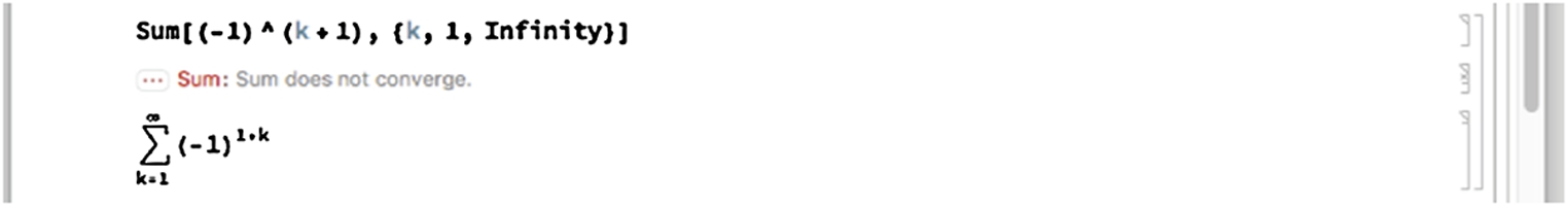
For (b), we have a telescoping series. Using partial fractions,
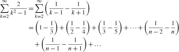
we see that the nth partial sum is given by
and ![]() as
as ![]() so the series converges to 3/2:
so the series converges to 3/2:

We perform the same steps with Mathematica using Sum, Apart, and Limit.
![]()
![]()
![]()
![]()
![]()
![]()
(c) A series of the form ![]() is called a geometric series. We compute the nth partial sum of the geometric series with Sum.
is called a geometric series. We compute the nth partial sum of the geometric series with Sum.
![]()
![]()
When using Limit to determine the limit of ![]() as
as ![]() , we see that Mathematica returns the limit unevaluated because Mathematica does not know the value of r.
, we see that Mathematica returns the limit unevaluated because Mathematica does not know the value of r.
![]()
![]()
In fact, the geometric series diverges if ![]() and converges if
and converges if ![]() . Observe that if we simply compute the sum with Sum, Mathematica returns
. Observe that if we simply compute the sum with Sum, Mathematica returns ![]() which is correct if
which is correct if ![]() but incorrect if
but incorrect if ![]() .
.
![]()
![]()
However, the result of entering
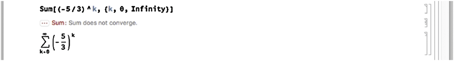
is correct because the series ![]() is geometric with
is geometric with ![]() and, consequently, diverges. Similarly,
and, consequently, diverges. Similarly,
![]()
1
is correct because ![]() is geometric with
is geometric with ![]() and
and ![]() so the series 0.999… converges to
so the series 0.999… converges to
□
3.4.3 Convergence Tests
Frequently used convergence tests for infinite series are stated in the following theorems. Note that the infinite series ![]() converges absolutely means that
converges absolutely means that ![]() converges. If an infinite series converges absolutely, it converges. If a series converges, but does not converge absolutely, we say that the series conditionally converges.
converges. If an infinite series converges absolutely, it converges. If a series converges, but does not converge absolutely, we say that the series conditionally converges.
The alternating harmonic series, ![]() is an example of a series that converges conditionally. It is a good exercise to show that the alternating harmonic series converges to
is an example of a series that converges conditionally. It is a good exercise to show that the alternating harmonic series converges to ![]() . On the other hand, the harmonic series,
. On the other hand, the harmonic series, ![]() diverges to +∞.
diverges to +∞.
Theorem 3.8
The Divergence Test
Let ![]() be an infinite series. If
be an infinite series. If ![]() , then
, then ![]() diverges.
diverges.
Theorem 3.9
The Integral Test
Let ![]() be an infinite series with positive terms. If
be an infinite series with positive terms. If ![]() is a decreasing continuous function for which
is a decreasing continuous function for which ![]() for all k, then
for all k, then ![]() and
and ![]() either both converge or both diverge.
either both converge or both diverge.
Theorem 3.10
The Ratio Test
Let ![]() be an infinite series and let
be an infinite series and let ![]() .
.
1. If ![]() ,
, ![]() converges absolutely.
converges absolutely.
2. If ![]() ,
, ![]() diverges.
diverges.
3. If ![]() , the Ratio Test is inconclusive.
, the Ratio Test is inconclusive.
Theorem 3.11
The Root Test
Let ![]() be an infinite series and let
be an infinite series and let ![]() .
.
1. If ![]() ,
, ![]() converges absolutely.
converges absolutely.
2. If ![]() ,
, ![]() diverges.
diverges.
3. If ![]() , the Root Test is inconclusive.
, the Root Test is inconclusive.
Theorem 3.12
The Limit Comparison Test
Let ![]() and
and ![]() be infinite series with positive terms and let
be infinite series with positive terms and let ![]() . If
. If ![]() , then either both series converge or both series diverge.
, then either both series converge or both series diverge.
Example 3.51
Determine whether each series converges or diverges. (a) ![]() ; (b)
; (b) ![]() ; (c)
; (c) ![]() ; (d)
; (d) ![]() ; (e)
; (e) ![]() ; (f)
; (f) ![]() .
.
Solution
(a) Using Limit, we see that the limit of the terms is ![]() so the series diverges by the Divergence Test, Theorem 3.8.
so the series diverges by the Divergence Test, Theorem 3.8.
![]()
e
It is a very good exercise to show that the limit of the terms of the series is e by hand. Let ![]() . Take the logarithm of each side of this equation and apply L'Hôpital's rule:
. Take the logarithm of each side of this equation and apply L'Hôpital's rule:
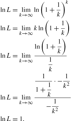
Exponentiating yields ![]() .
.
(b) A series of the form ![]() (
(![]() ) is called a p-series. Let
) is called a p-series. Let ![]() . Then,
. Then, ![]() is continuous and decreasing for
is continuous and decreasing for ![]() ,
, ![]() and
and

so the p-series converges if ![]() and diverges if
and diverges if ![]() . If
. If ![]() , the series
, the series ![]() is called the harmonic series. Observe that Mathematica's result is given in terms of a “conditional expression.” In this example, the interpretation is that
is called the harmonic series. Observe that Mathematica's result is given in terms of a “conditional expression.” In this example, the interpretation is that ![]() provided that the real part of p is greater than 1.
provided that the real part of p is greater than 1.
![]()
![]()
![]()
(c) Let ![]() . Then,
. Then, ![]() and
and ![]() is decreasing for
is decreasing for ![]() because
because ![]() for
for ![]() .
.
![]()
![]()
![]()
![]()
![]()
Using Integrate, we see that the improper integral ![]() converges.
converges.
![]()
![]()
![]()
0.579592
Thus, by the Integral Test, Theorem 3.9, we conclude that the series converges. Note that when applying the Integral Test, if the improper integral converges its value is not the value of the sum of the series. In this case, we see that Mathematica is able to evaluate the sum with Sum and the series converges to 3/4.
![]()
![]()
(d) If ![]() contains factorial functions, the Ratio Test is often a good first test to try. After defining
contains factorial functions, the Ratio Test is often a good first test to try. After defining ![]() we compute
we compute
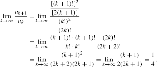
Because ![]() , the series converges by the Ratio Test. We confirm these results with Mathematica.
, the series converges by the Ratio Test. We confirm these results with Mathematica.
![]()
![]()
![]()
![]()
![]()
We illustrate that we can evaluate the sum using Sum and approximate it with N as follows.
![]()
![]()
![]()
0.7364
(e) Because
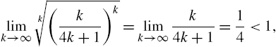
the series converges by the Root Test.
![]()
![]()
![]()
As with (d), we can approximate the sum with N and Sum.
![]()
![]()
![]()
0.265757
(f) We use the Limit Comparison Test and compare the series to ![]() , which diverges because it is a p-series with
, which diverges because it is a p-series with ![]() . Because
. Because
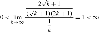
and the harmonic series diverges, the series diverges by the Limit Comparison Test.
![]()
![]()
![]()
1 □
3.4.4 Alternating Series
An alternating series is a series of the form
where ![]() is a sequence with positive terms.
is a sequence with positive terms.
Theorem 3.13
Alternating Series Test
If ![]() is decreasing and
is decreasing and ![]() , the alternating series (3.27) converges.
, the alternating series (3.27) converges.
Definition 3.3
The alternating series (3.27) converges absolutely if ![]() converges.
converges.
Example 3.52
Determine whether each series converges or diverges. If the series converges, determine whether the convergence is conditional or absolute. (a) ![]() ; (b)
; (b) ![]() ; (c)
; (c) ![]() .
.
Solution
(a) Because ![]() is decreasing and
is decreasing and ![]() as
as ![]() , the series converges. The series does not converge absolutely because the harmonic series diverges. Hence,
, the series converges. The series does not converge absolutely because the harmonic series diverges. Hence, ![]() , which is called the alternating harmonic series, converges conditionally. We see that this series converges to
, which is called the alternating harmonic series, converges conditionally. We see that this series converges to ![]() with Sum.
with Sum.
![]()
![]()
![]()
(b) We test for absolute convergence first using the Ratio Test. Because
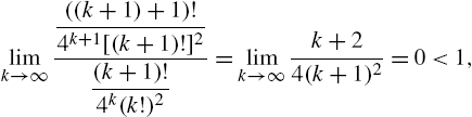
![]()
![]()
![]()
![]()
0
the series converges absolutely by the Ratio Test. Absolute convergence implies convergence so the series converges.
(c) Because ![]() ,
, ![]() does not exist, so the series diverges by the Divergence Test. We confirm that the limit of the terms is not zero with Limit.
does not exist, so the series diverges by the Divergence Test. We confirm that the limit of the terms is not zero with Limit.
![]()
![]()
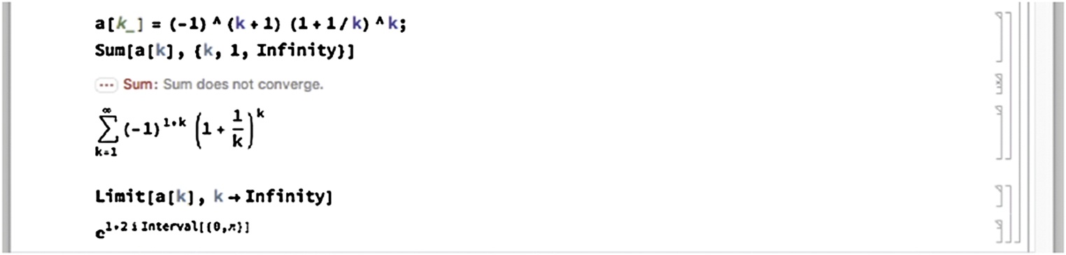
![]()
![]() □
□
3.4.5 Power Series
Let ![]() be a number. A power series in
be a number. A power series in ![]() is a series of the form
is a series of the form

A fundamental problem is determining the values of x, if any, for which the power series converges, the interval of convergence.
Theorem 3.15
For the power series (3.28), exactly one of the following is true.
1. The power series converges absolutely for all values of x. The interval of convergence is ![]() .
.
2. There is a positive number r so that the series converges absolutely if ![]() . The series may or may not converge at
. The series may or may not converge at ![]() and
and ![]() . The interval of convergence will be one of
. The interval of convergence will be one of ![]() ,
, ![]() ,
, ![]() , or
, or ![]() .
.
3. The series converges only if ![]() . The interval of convergence is
. The interval of convergence is ![]() .
.
Example 3.53
Determine the interval of convergence for each of the following power series. (a) ![]() ; (b)
; (b) ![]() ; (c)
; (c) ![]() .
.
Solution
(a) We test for absolute convergence first using the Ratio Test. Because
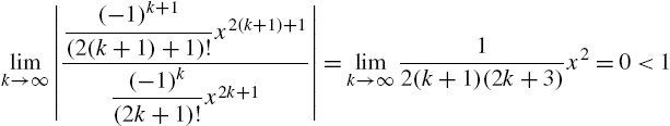
![]()
![]()
![]()
![]()
0
for all values of x, we conclude that the series converges absolutely for all values of x; the interval of convergence is ![]() . In fact, we will see later that this series converges to
. In fact, we will see later that this series converges to ![]() :
:
which means that the partial sums of the series converge to ![]() . Graphically, we can visualize this by graphing partial sums of the series together with the graph of
. Graphically, we can visualize this by graphing partial sums of the series together with the graph of ![]() . Note that the partial sums of a series are a recursively defined function:
. Note that the partial sums of a series are a recursively defined function: ![]() ,
, ![]() . We use this observation to define p to be the nth partial sum of the series. We use the form p[x_,n_]:=p[x,n]=... so that Mathematica “remembers” the partial sums computed. That is, once p[x,3] is computed, Mathematica need not recompute p[x,3] when computing p[x,4].
. We use this observation to define p to be the nth partial sum of the series. We use the form p[x_,n_]:=p[x,n]=... so that Mathematica “remembers” the partial sums computed. That is, once p[x,3] is computed, Mathematica need not recompute p[x,3] when computing p[x,4].
In Fig. 3.54 we graph ![]() together with
together with ![]() for
for ![]() , 5, and 10. In the graphs, notice that as n increases, the graphs of
, 5, and 10. In the graphs, notice that as n increases, the graphs of ![]() more closely resemble the graph of
more closely resemble the graph of ![]() .
.
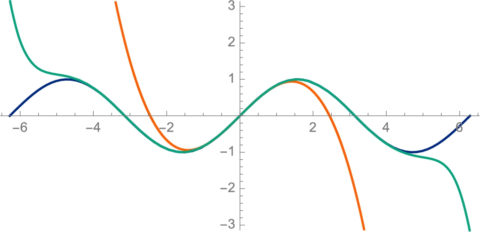 together with the graphs of p1(x), p5(x), and p10(x).
![]()
![]()
![]()
![]()
![]()
![]()
![]()
![]()
![]()
We use Manipulate to investigate how n affects the situation with (see Fig. 3.55)
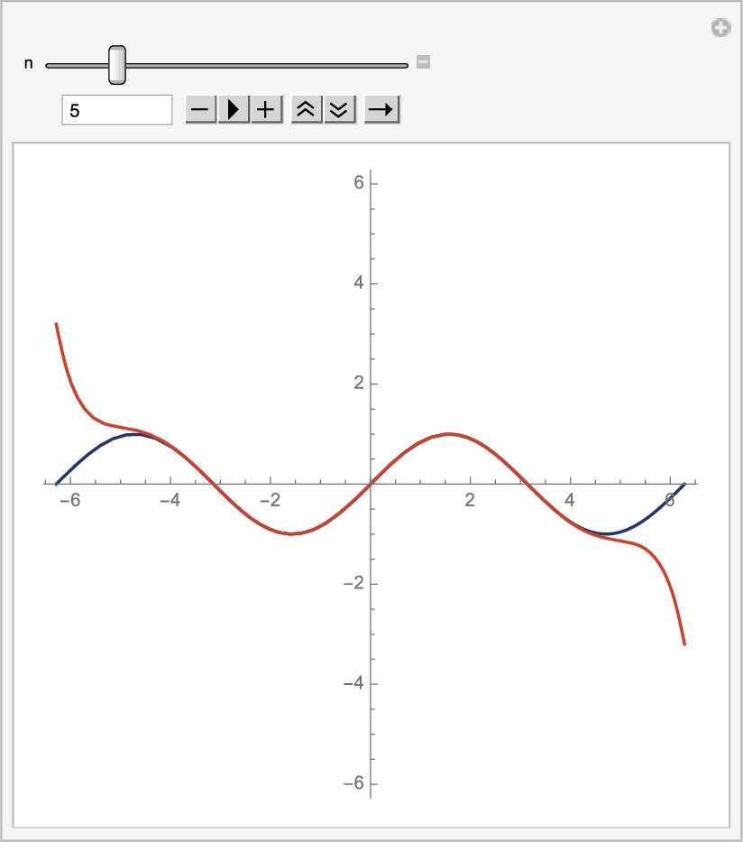
![]()
![]()
![]()
![]()
(b) As in (a), we test for absolute convergence first using the Ratio Test:
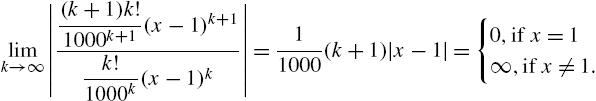
![]()
![]()
![]()
![]()
![]()
Be careful of your interpretation of the result of the Limit command because Mathematica does not consider the case ![]() separately: if
separately: if ![]() the limit is 0. Because
the limit is 0. Because ![]() the series converges by the Ratio Test.
the series converges by the Ratio Test.
The series converges only if ![]() ; the interval of convergence is {1}. You should observe that if you graph several partial sums for “small” values of n, you might incorrectly conclude that the series converges. (c) Use the Ratio Test to check absolute convergence first:
; the interval of convergence is {1}. You should observe that if you graph several partial sums for “small” values of n, you might incorrectly conclude that the series converges. (c) Use the Ratio Test to check absolute convergence first:
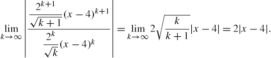
By the Ratio Test, the series converges absolutely if ![]() . We solve this inequality for x with Reduce to see that
. We solve this inequality for x with Reduce to see that ![]() if
if ![]() .
.
![]()
![]()
![]()
![]()
![]()
![]()
Use Reduce to solve the inequality.
![]()
![]()
![]()
From the output, we see that for real values of x, the inequality is satisfied for ![]() . We check
. We check ![]() and
and ![]() separately. If
separately. If ![]() , the series becomes
, the series becomes ![]() , which converges conditionally.
, which converges conditionally.
![]()
![]()
On the other hand, if ![]() ,
,
![]()
![]()
the series is ![]() , which diverges. We conclude that the interval of convergence is
, which diverges. We conclude that the interval of convergence is ![]() . □
. □
3.4.6 Taylor and Maclaurin Series
Let ![]() be a function with derivatives of all orders at
be a function with derivatives of all orders at ![]() . The Taylor series for
. The Taylor series for ![]() about
about ![]() is
is
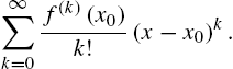
The Maclaurin series for ![]() is the Taylor series for
is the Taylor series for ![]() about
about ![]() . If
. If ![]() has derivatives up to at least order n at
has derivatives up to at least order n at ![]() , the nth degree Taylor polynomial for
, the nth degree Taylor polynomial for ![]() about
about ![]() is
is

The nth degree Maclaurin polynomial for ![]() is the nth degree Taylor polynomial for
is the nth degree Taylor polynomial for ![]() about
about ![]() . Generally, finding Taylor and Maclaurin series using the definition is a tedious task at best.
. Generally, finding Taylor and Maclaurin series using the definition is a tedious task at best.
Example 3.54
Find the first few terms of (a) the Maclaurin series and (b) the Taylor series about ![]() for
for ![]() .
.
Solution
(a) After defining ![]() , we use Table together with /. and D to compute
, we use Table together with /. and D to compute ![]() for
for ![]() , 1, …, 8.
, 1, …, 8.
![]()
![]()
![]()
![]()
![]()
![]()
To see these results in tabular form, enter
![]()
For length considerations, the resulting output is not shown here. Another way of approaching the problem is to use Manipulate. See Fig. 3.56.
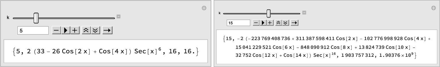
![]()
![]()
Using the values in the table or from the Manipulate object, we apply the definition to see that the Maclaurin series is
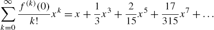
For (b), we repeat (a) using ![]() instead of
instead of ![]()
![]()
![]()
and then apply the definition to see that the Taylor series about ![]() is
is
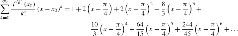
From the series, we can see various Taylor and Maclaurin polynomials. For example, the third Maclaurin polynomial is
and the 4th degree Taylor polynomial about ![]() is
is
See Fig. 3.57. □
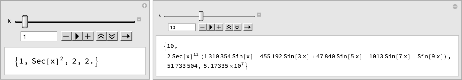
The command Series[f[x],{x,x0,n}] computes (3.29) to (at least) order ![]() . Because of the O-term in the result that represents the terms that are omitted from the power series for
. Because of the O-term in the result that represents the terms that are omitted from the power series for ![]() expanded about the point
expanded about the point ![]() , the result of entering a Series command is not a function that can be evaluated if x is a particular number. We remove the remainder (O-) term of the power series Series[f[x],{x,x0,n}] with the command Normal and can then evaluate the resulting polynomial for particular values of x.
, the result of entering a Series command is not a function that can be evaluated if x is a particular number. We remove the remainder (O-) term of the power series Series[f[x],{x,x0,n}] with the command Normal and can then evaluate the resulting polynomial for particular values of x.
Example 3.55
Find the first few terms of the Taylor series for ![]() about
about ![]() . (a)
. (a) ![]() ,
, ![]() ; (b)
; (b) ![]() ,
, ![]() .
.
Solution
Entering
![]()
![]()
computes the Maclaurin series to order 4. Entering
![]()
![]()
computes the Maclaurin series to order 14. In this case, the Maclaurin series for ![]() converges to
converges to ![]() for all real x. To graphically see this, we define the function p. Given n, p[n] returns the Maclaurin polynomial of degree n for
for all real x. To graphically see this, we define the function p. Given n, p[n] returns the Maclaurin polynomial of degree n for ![]() .
.
![]()
![]()
![]()
We then graph ![]() together with the Maclaurin polynomial of degree
together with the Maclaurin polynomial of degree ![]() , 4, 8, and 16 on the interval
, 4, 8, and 16 on the interval ![]() in Fig. 3.58. Notice that as n increases, the graph of the Maclaurin polynomial more closely resembles the graph of
in Fig. 3.58. Notice that as n increases, the graph of the Maclaurin polynomial more closely resembles the graph of ![]() . We would see the same pattern if we increased the length of the interval and the value of n.
. We would see the same pattern if we increased the length of the interval and the value of n.
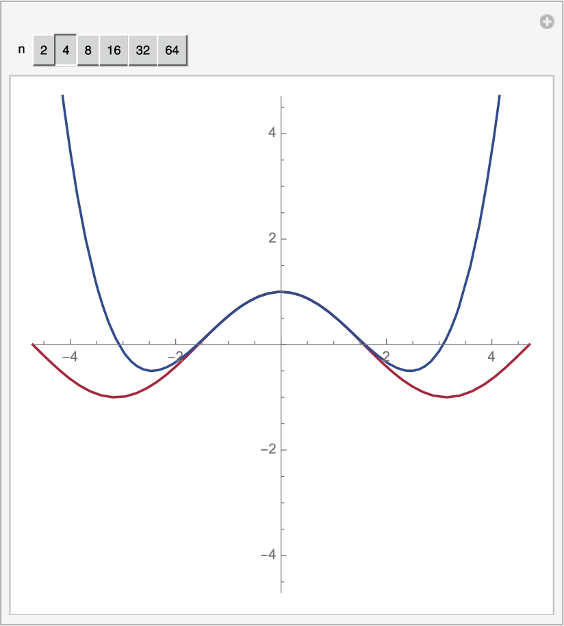 together with plots of several of its Maclaurin polynomials (University of Pennsylvania colors).
![]()
![]()
![]()
![]()
(b) After defining ![]() , we compute the first 10 terms of the Taylor series for
, we compute the first 10 terms of the Taylor series for ![]() about
about ![]() with Series.
with Series.
![]()
![]()
![]()
In this case, the pattern for the series is relatively easy to see: the Taylor series for ![]() about
about ![]() is
is
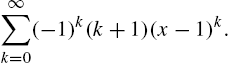
This series converges absolutely if

or ![]() . The series diverges if
. The series diverges if ![]() and
and ![]() . In this case, the series converges to
. In this case, the series converges to ![]() on the interval
on the interval ![]() .
.
![]()
![]()
![]()
![]()
![]()
![]()
![]()
To see this, we use Manipulate to graph ![]() together with the Taylor polynomial for
together with the Taylor polynomial for ![]() about
about ![]() of degree n for large n. Regardless of the size of n, the graphs of
of degree n for large n. Regardless of the size of n, the graphs of ![]() and the Taylor polynomial closely resemble each other on the interval
and the Taylor polynomial closely resemble each other on the interval ![]() – but not at the endpoints or outside the interval. (See Fig. 3.59.)
– but not at the endpoints or outside the interval. (See Fig. 3.59.)
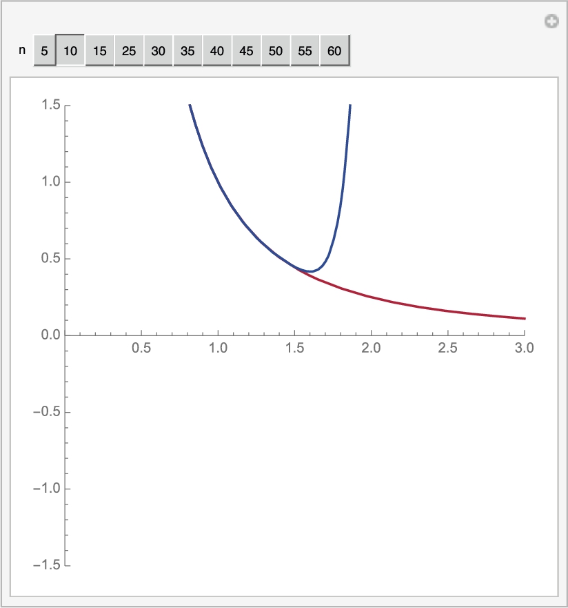
![]()
![]()
![]()
![]()
![]() □
□
3.4.7 Taylor's Theorem
Taylor's theorem states the relationship between ![]() and the Taylor series for
and the Taylor series for ![]() about
about ![]() .
.
Theorem 3.16
Taylor's Theorem
Let ![]() have (at least)
have (at least) ![]() derivatives on an interval I containing
derivatives on an interval I containing ![]() . Then, for every number
. Then, for every number ![]() , there is a number z between x and
, there is a number z between x and ![]() so that
so that
where ![]() is given by equation (3.30) and
is given by equation (3.30) and
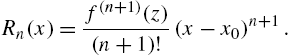
Example 3.56
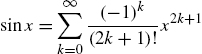
Solution
Let ![]() . Then, for each value of x, there is a number z between 0 and x so that
. Then, for each value of x, there is a number z between 0 and x so that ![]() where
where ![]() and
and ![]() . Regardless of the value of n,
. Regardless of the value of n, ![]() is one of
is one of ![]() ,
, ![]() ,
, ![]() , or
, or ![]() , which are all bounded by 1. Then,
, which are all bounded by 1. Then,

and ![]() as
as ![]() for all real values of x.
for all real values of x.
You should remember that the number z in ![]() is guaranteed to exist by Taylor's theorem. However, from a practical point of view, you would rarely (if ever) need to compute the z value for a particular x value.
is guaranteed to exist by Taylor's theorem. However, from a practical point of view, you would rarely (if ever) need to compute the z value for a particular x value.
For illustrative purposes, we show the difficulties. Suppose we wish to approximate ![]() using the Maclaurin polynomial of degree 4,
using the Maclaurin polynomial of degree 4, ![]() , for
, for ![]() . The fourth remainder is
. The fourth remainder is ![]() .
.
The Maclaurin polynomial of degree 4 for ![]() is
is ![]()
![]() .
.
![]()
![]()
![]()
![]()
If ![]() there is a number z between 0 and
there is a number z between 0 and ![]() so that
so that

which shows us that the maximum the error can be is ![]() .
.
![]()
![]()
Abstractly, the exact error can be computed. By Taylor's theorem, z satisfies

We graph the right-hand side of this equation with Plot in Fig. 3.60. The exact value of z is the z-coordinate of the point where the graph intersects the z-axis.
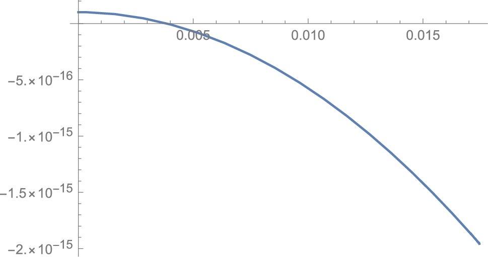
![]()
![]()
![]()
![]()
![]()
![]()
![]()
![]()
![]()
![]()
We can use FindRoot to approximate z, if we increase the number of digits carried in floating point calculations with WorkingPrecision.
![]()
![]()
Alternatively, we can compute the exact value of z with Solve
![]()
![]()
![]()
![]()
and then approximate the result with N.
![]()
![]()
![]() □
□
Example 3.57
Newton's Approximation of π.
Newton's Approximation of π is a fascinating combination of calculus, infinite series, and geometry. Newton began the approximation after proving the Binomial Theorem.
Theorem 3.17
Binomial Theorem
We use Series to find the first few terms of the Binomial series.
![]()
![]()
Newton then used the Binomial series to find the first few terms of the series for ![]() .
.
![]()
![]()
In Fig. 3.61, observe that the series quickly converges to ![]() if x is small. He used this observation to use the series to approximate
if x is small. He used this observation to use the series to approximate ![]() by observing
by observing
and substituting ![]() into the first few terms of the series.
into the first few terms of the series.
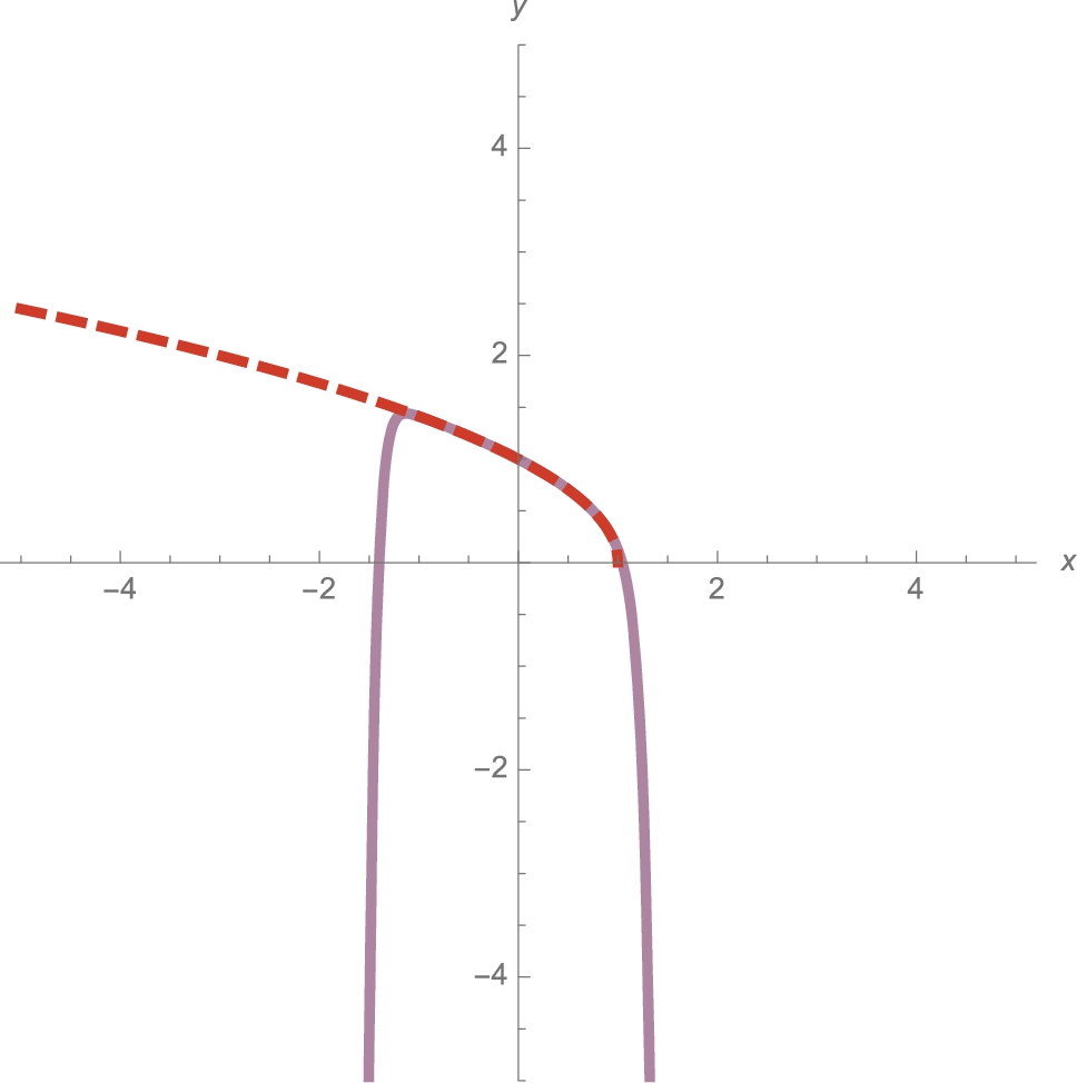
 converges quickly to when x is small (Virginia Polytechnic Institute & State University colors).
![]()
![]()
![]()
Next, Newton looked at the circle ![]() with center at
with center at ![]() and radius 1/2. Refer to Fig. 3.62.
and radius 1/2. Refer to Fig. 3.62.
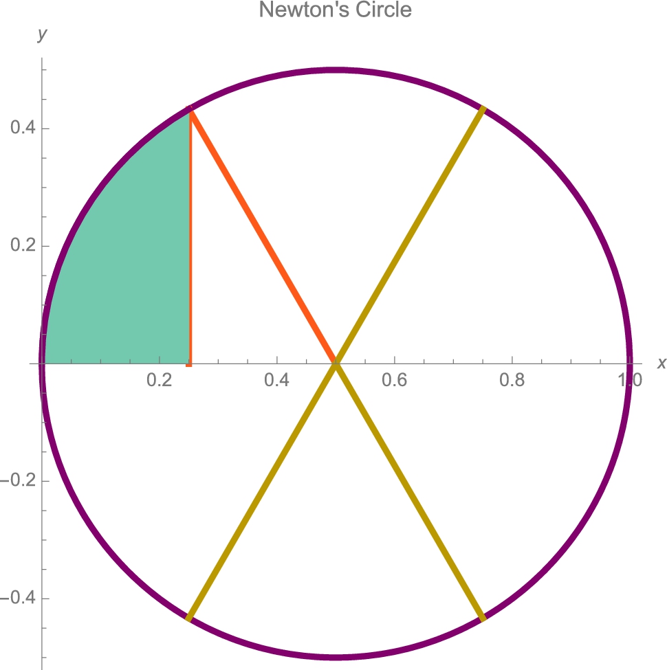
 .
.
![]()
![]()
![]()
![]()
![]()
![]()
![]()
![]()
![]()
![]()
![]()
Newton understood that the area of a circle with radius r is ![]() so it followed that the area of Newton's circle is
so it followed that the area of Newton's circle is ![]() . Moreover, the area of the sector formed by the green region and the orange triangle is 1/6th the area of the circle so the area of the sector is
. Moreover, the area of the sector formed by the green region and the orange triangle is 1/6th the area of the circle so the area of the sector is ![]() . The orange triangle has width 1/4 and height
. The orange triangle has width 1/4 and height ![]() so the orange triangle has area
so the orange triangle has area
Because the top half of the circle is given by ![]() , the area of the green region, R, is
, the area of the green region, R, is ![]() . Newton then added and solved for π.
. Newton then added and solved for π.

Newton already had an excellent approximation of ![]() as described above. Thus, to obtain an excellent approximation of π he needed only to find an excellent approximation of
as described above. Thus, to obtain an excellent approximation of π he needed only to find an excellent approximation of ![]() . To obtain it, he started with his power series for
. To obtain it, he started with his power series for ![]() and then observed that for
and then observed that for ![]() ,
, ![]() . With that in mind, he decided to take his power series for
. With that in mind, he decided to take his power series for ![]() and multiply it by
and multiply it by ![]() to obtain a series that he predicted would converge to
to obtain a series that he predicted would converge to ![]() . Newton was right and it worked!
. Newton was right and it worked!
![]()
![]()
He then integrated his series (which was no longer a power series) term-by-term
![]()
![]()
and evaluated it if ![]() to obtain his approximation of
to obtain his approximation of ![]() .
.
There is no need to show the evaluation of the series if ![]() because the value of the series if
because the value of the series if ![]() is 0.
is 0.
![]()
![]()
We use N to obtain a numerical result.
![]()
0.0767731
We use Table to illustrate the steps Newton carried out by hand. In the first column, k, in the second column, the kth term of the series for ![]() centered at
centered at ![]() , in the third column, an antiderivative of the kth term of the series for
, in the third column, an antiderivative of the kth term of the series for ![]() centered at
centered at ![]() , and in the fourth column, the value of the antiderivative of the kth term of the series for
, and in the fourth column, the value of the antiderivative of the kth term of the series for ![]() centered at
centered at ![]() evaluated at
evaluated at ![]() .
.
![]()
![]()
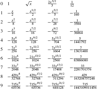
Thus, Newton's approximation of π, ![]() using his approximations of
using his approximations of ![]() was given by
was given by
![]()
![]()
We use N to approximate ![]() .
.
![]()
![]()
3.1415926683631729578
When we compare Newton's approximation of π to our present day approximation of π, it is truly remarkable that Newton's approximation was accurate to seven decimal places (to the right of the decimal point).
![]()
3.1415926535897932385
There are volumes of literature about the history of π, its applications, and how to efficiently and accurately approximate π (as well as other irrational and transcendental numbers).
Example 3.58
Determine whether the following series converge or diverge: (a) ![]() ; (b)
; (b) ![]() ; (c)
; (c) ![]() ; (d)
; (d) ![]() .
.
Solution
To determine whether each series converges or diverges, we use the Ratio Test. For (a), we see that ![]() . Because
. Because ![]() , the series converges (absolutely).
, the series converges (absolutely).
![]()
![]()
![]()
![]()
![]()
![]()
In fact, in 1997, David Bailey, Peter Borwein, and Simon Plouffe (BBP) proved that
Notice that the second partial sum is accurate to three decimal places,
![]()
3.141422466
and the seventh partial sum is accurate to ten decimal places.
![]()
3.14159265357288
![]()
3.14159265358979
Interestingly, in 2013, Fabrice Bellard improved on the BBP equation and proved that

(b) Using the Ratio Test, we see that the series converges because the limit of the ratio of successive terms is ![]() :
: ![]() .
.
![]()
![]()
![]()
![]()
![]()
![]()
Newton proved that this series converges to ![]() :
:

Observe that the “patterns” of the terms of this series are much easier to see than in the example illustrating Newton's approximation of π using integral calculus, infinite series, and Euclidean geometry. You can use the 31st partial sum of this series to approximate ![]() to 10 decimal places.
to 10 decimal places.
![]()
1.570796327
![]()
1.570796327
(c) Using the Ratio Test, we see that
![]()
![]()
![]()
![]()
![]()
![]()
![]() so the series converges absolutely. This series that was introduced by Srinivasa Ramanujan around 1910 converges to
so the series converges absolutely. This series that was introduced by Srinivasa Ramanujan around 1910 converges to ![]() :
:

As with the other series in this example, the convergence is quick.
![]()
0.318309886183790671537767
![]()
0.318309886183790671537768
With just the third partial sum of the series, we see that it approximates ![]() to 23 decimal places.
to 23 decimal places.
(d) Using the Ratio Test, we see that the series converges. This formulation of π was introduced by brothers David Chudnosky and Gregory Chudnosky in 1989:
![]()
![]()
![]()
![]()
![]()
![]()
The series converges very quickly. Using the third partial sum, we see that it yields an approximation of ![]() accurate to 42 decimal places.
accurate to 42 decimal places.
![]()
0.318309886183790671537767526745028724068919
![]()
0.318309886183790671537767526745028724068919
To use the Chudnosky's series to approximate π, we first rewrite it as
Now let ![]() and
and ![]() . Then (3.33) becomes
. Then (3.33) becomes

and reciprocating gives us
Observe that ![]() ,
, ![]() , and
, and
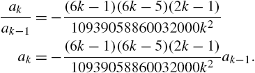
Then, if we let ![]() ,
,
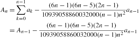
and if we let ![]() ,
, ![]() . Then, we approximate π with
. Then, we approximate π with ![]() .
.
![]()
![]()
![]()
![]()
![]()
![]()
![]()
![]()
![]()
We illustrate the quick convergence using ![]() and
and ![]() . Observe that the approximation gives us an approximation of π accurate to at least 155 digits.
. Observe that the approximation gives us an approximation of π accurate to at least 155 digits.
![]()
![]()
![]()
![]() □
□
Closely related to these series is the Madhava–Leibniz series, ![]() . It is a good exercise to verify that the first 21 terms of the Madhava–Leibniz series compute an approximation of π accurate to eleven decimal places.
. It is a good exercise to verify that the first 21 terms of the Madhava–Leibniz series compute an approximation of π accurate to eleven decimal places.
3.4.8 Other Series
In calculus, we learn that the power series ![]() is differentiable and integrable on its interval of convergence. However, for series that are not power series this result is not generally true. For example, in more advanced courses, we learn that the function
is differentiable and integrable on its interval of convergence. However, for series that are not power series this result is not generally true. For example, in more advanced courses, we learn that the function

is continuous for all values of x but nowhere differentiable. We can use Mathematica to help us see why this function is not differentiable. Let
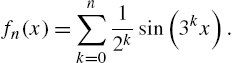
Notice that ![]() is defined recursively by
is defined recursively by ![]() and
and ![]() . We use Mathematica to recursively define
. We use Mathematica to recursively define ![]() .
.
![]()
![]()
![]()
We define ![]() using the form
using the form
f[n_]:=f[n]=...
so that Mathematica “remembers” the values it computes. Thus, to compute f[5], Mathematica uses the previously computed values, namely f[4], to compute f[5]. Note that we can produce the same results by defining ![]() with the command
with the command
f[n_]:=...
However, the disadvantage of defining ![]() in this manner is that Mathematica does not “remember” the previously computed values and thus takes longer (and uses more memory) to compute
in this manner is that Mathematica does not “remember” the previously computed values and thus takes longer (and uses more memory) to compute ![]() for larger values of n.
for larger values of n.
Next, we use Table to generate ![]() ,
, ![]() ,
, ![]() , and
, and ![]() .
.
![]()
We now graph each of these functions and show the results as a graphics array with GraphicsGrid in Fig. 3.63. (Note that you do not need to include the option DisplayFunction->Identity to suppress the resulting output unless you forget to include the semi-colon at the end of the command.)
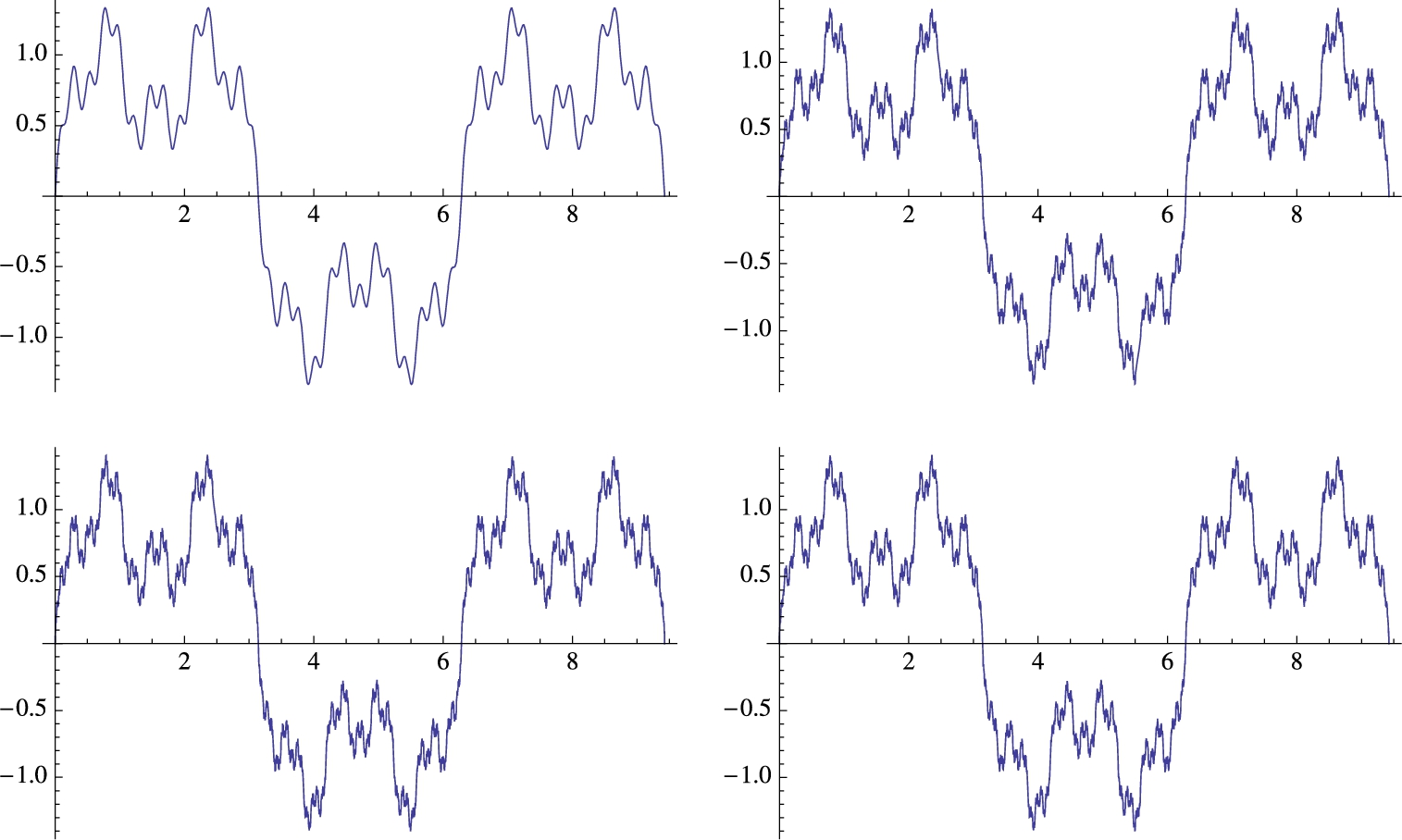
![]()
![]()
![]()
![]()
From these graphs, we see that for large values of n, the graph of ![]() , although actually smooth, appears “jagged” and thus we might suspect that
, although actually smooth, appears “jagged” and thus we might suspect that ![]()
![]() is indeed continuous everywhere but nowhere differentiable.
is indeed continuous everywhere but nowhere differentiable.
3.5 Multi-Variable Calculus
Mathematica is useful in investigating functions involving more than one variable. In particular, the graphical analysis of functions that depend on two (or more) variables is enhanced with the help of Mathematica's graphics capabilities.
3.5.1 Limits of Functions of Two Variables
Mathematica's graphics and numerical capabilities are helpful in investigating limits of functions of two variables.
Example 3.59
Show that the limit ![]() does not exist.
does not exist.
Solution
We begin by defining ![]() . Next, we use Plot3D to graph
. Next, we use Plot3D to graph ![]() for
for ![]() and
and ![]() . ContourPlot is used to graph several level curves on the same rectangle. (See Fig. 3.64.) (To define a function of two variables,
. ContourPlot is used to graph several level curves on the same rectangle. (See Fig. 3.64.) (To define a function of two variables, ![]() , enter f[x_,y_]=expression in x and y. Plot3D[f[x,y],{a,x,b},{y,c,d}] generates a basic graph of
, enter f[x_,y_]=expression in x and y. Plot3D[f[x,y],{a,x,b},{y,c,d}] generates a basic graph of ![]() for
for ![]() and
and ![]() )
)
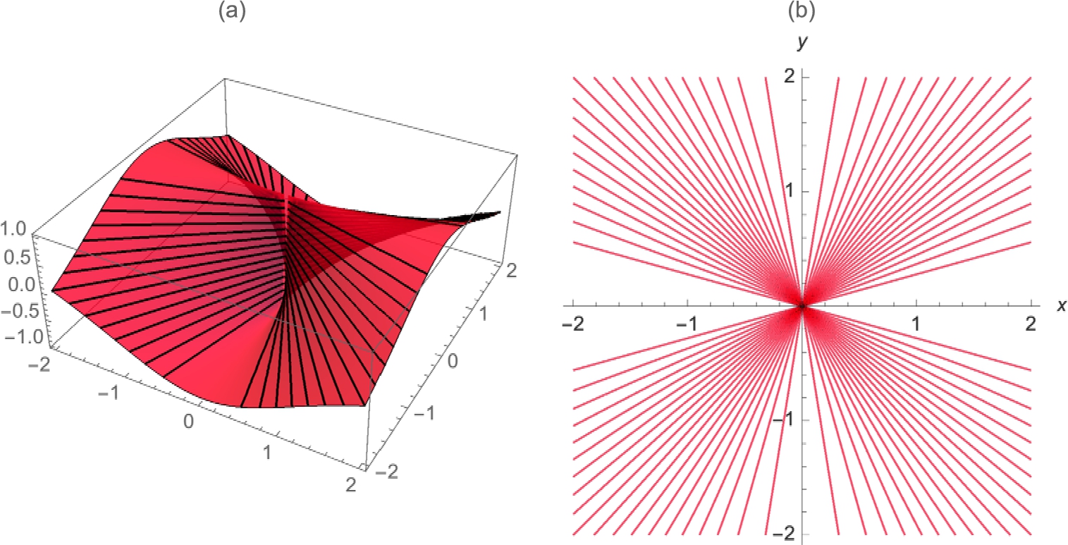
![]()
![]()
![]()
![]()
![]()
![]()
![]()
![]()
![]()
![]()
From the graph of the level curves, we suspect that the limit does not exist because we see that near ![]() ,
, ![]() attains many different values. We obtain further evidence that the limit does not exist by computing the value of
attains many different values. We obtain further evidence that the limit does not exist by computing the value of ![]() for various points chosen randomly near
for various points chosen randomly near ![]() . We use Table and RandomReal to generate 10 ordered pairs
. We use Table and RandomReal to generate 10 ordered pairs ![]() for x and y “close to” 0. Because RandomReal is included in the calculation, your results will almost certainly be different from those here.
for x and y “close to” 0. Because RandomReal is included in the calculation, your results will almost certainly be different from those here.
![]()
![]()
Next, we define a function g that given an ordered pair ![]() ({x,y} in Mathematica),
({x,y} in Mathematica), ![]() returns the ordered triple
returns the ordered triple ![]() ({x,y,f[x,y]} in Mathematica).
({x,y,f[x,y]} in Mathematica).
![]()
![]()
We then use Map to apply g to the list pts.
![]()

From the third column, we see that ![]() does not appear to approach any particular value for points chosen randomly near
does not appear to approach any particular value for points chosen randomly near ![]() . In fact, along the line
. In fact, along the line ![]() we see that
we see that ![]() . Hence as
. Hence as ![]() along
along ![]() ,
, ![]() . Thus,
. Thus, ![]() does not have a limit as
does not have a limit as ![]() .
.
We choose lines of the form ![]() because near
because near ![]() the level curves of
the level curves of ![]() look like lines of the form
look like lines of the form ![]() .
.
![]()
![]()
![]()
![]()
![]()
1
0
![]() □
□
In some cases, you can establish that a limit does not exist by converting to polar coordinates. For example, in polar coordinates, ![]() becomes
becomes ![]()
![]()
![]()
and
depends on θ.
3.5.2 Partial and Directional Derivatives
Partial derivatives of functions of two or more variables are computed with Mathematica using D. For ![]() ,
,
1. D[f[x,y],x] computes ![]() ,
,
2. D[f[x,y],y] computes ![]() ,
,
3. D[f[x,y],{x,n}] computes ![]() ,
,
4. D[f[x,y],y,x] computes ![]() , and
, and
5. D[f[x,y],{x,n},{y,m}] computes ![]() .
.
6. You can use the ![]() button located on the BasicMathInput palette to create templates to compute partial derivatives.
button located on the BasicMathInput palette to create templates to compute partial derivatives.
The calculations are carried out similarly for functions of more than two variables.
Example 3.60
Calculate ![]() ,
, ![]() ,
, ![]() ,
, ![]() ,
, ![]() , and
, and ![]() if
if ![]() .
.
Solution
After defining ![]() ,
,
![]()
we illustrate the use of D to compute the partial derivatives. Entering
![]()
![]()
computes ![]() . Entering
. Entering
![]()
![]()
computes ![]() . Entering
. Entering
![]()
![]()
computes ![]() . Entering
. Entering
![]()
![]()
computes ![]() . Remember that under appropriate assumptions,
. Remember that under appropriate assumptions, ![]() . Entering
. Entering
![]()
![]()
computes ![]() . Entering
. Entering
![]()
![]()
computes ![]() . □
. □
The directional derivative of ![]() in the direction of the unit vector
in the direction of the unit vector ![]() is
is
provided that ![]() and
and ![]() both exist.
both exist.
The vectors i and j are defined by ![]() and
and ![]() .
.
If ![]() and
and ![]() both exist, the gradient of
both exist, the gradient of ![]() is the vector-valued function
is the vector-valued function
Notice that if ![]() ,
,
Let ![]() be a point in the domain of the differentiable function
be a point in the domain of the differentiable function ![]() . At
. At ![]() ,
, ![]() increases most rapidly in the direction of the gradient,
increases most rapidly in the direction of the gradient, ![]() , evaluated at
, evaluated at ![]() . Similarly,
. Similarly, ![]() decreases most rapidly in the direction of
decreases most rapidly in the direction of ![]() . Consequently, the gradient is perpendicular to the level curves of
. Consequently, the gradient is perpendicular to the level curves of ![]() .
.
StreamPlot[{f(x,y),g(x,y)},{x,a,b},{y,c,d}]
generates a stream plot of the vector field ![]() . Thus,
. Thus,
StreamPlot[{D[f[x,y],x],D[f[x,y],y]},{x,a,b},{y,c,d}]
generates a stream plot of the gradient of ![]() .
.
Example 3.61
Let ![]() . (a) Find
. (a) Find ![]() in the direction of
in the direction of ![]() . (b) Compute
. (b) Compute ![]() . (c) Find an equation of the line tangent to the graph of
. (c) Find an equation of the line tangent to the graph of ![]() at the point
at the point ![]() .
.
Solution
After defining ![]() , we graph
, we graph ![]() with Plot3D in Fig. 3.65, illustrating the PlotPoints, PlotRange, and ViewPoint options.
with Plot3D in Fig. 3.65, illustrating the PlotPoints, PlotRange, and ViewPoint options.
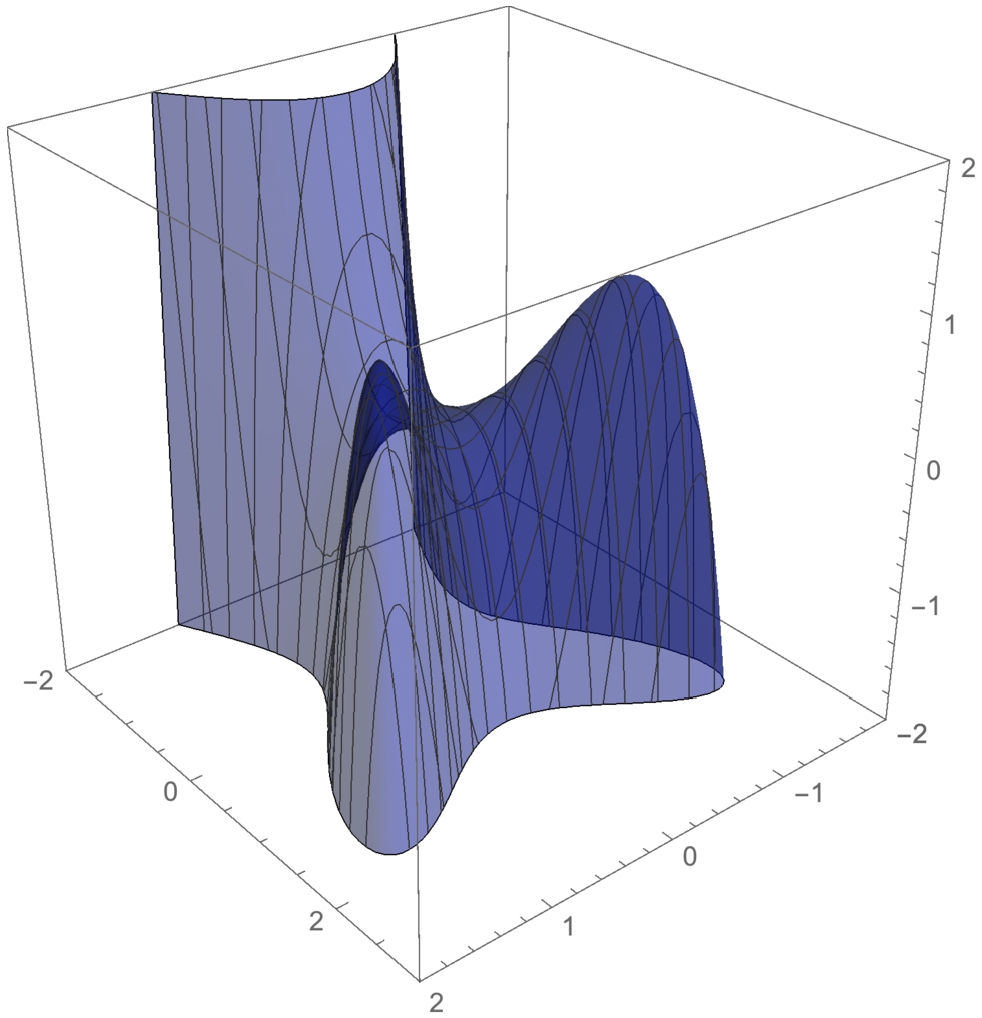
![]()
![]()
![]()
![]()
![]()
![]()
(a) A unit vector, u, in the same direction as v is
![]()
![]()
![]()
Then, ![]() , calculated in du.
, calculated in du.
![]()
![]()
![]()
![]()
(b) ![]() is calculated by evaluating du if
is calculated by evaluating du if ![]() and
and ![]() .
.
![]()
![]()
(c) The gradient is evaluated if ![]() and
and ![]() .
.
![]()
![]()
Generally, ![]() is perpendicular to the level curves of
is perpendicular to the level curves of ![]() , so
, so

is perpendicular to ![]() at the point
at the point ![]() . Thus, an equation of the line tangent to the graph of
. Thus, an equation of the line tangent to the graph of ![]() at the point
at the point ![]() is
is

which we solve for y with Solve. We confirm this result by graphing ![]() using ContourPlot in conf and then graphing the tangent line in tanplot. tanplot and conf are shown together with Show in Fig. 3.66.
using ContourPlot in conf and then graphing the tangent line in tanplot. tanplot and conf are shown together with Show in Fig. 3.66.
An equation of the line L containing ![]() and perpendicular to
and perpendicular to ![]() is
is ![]() .
.
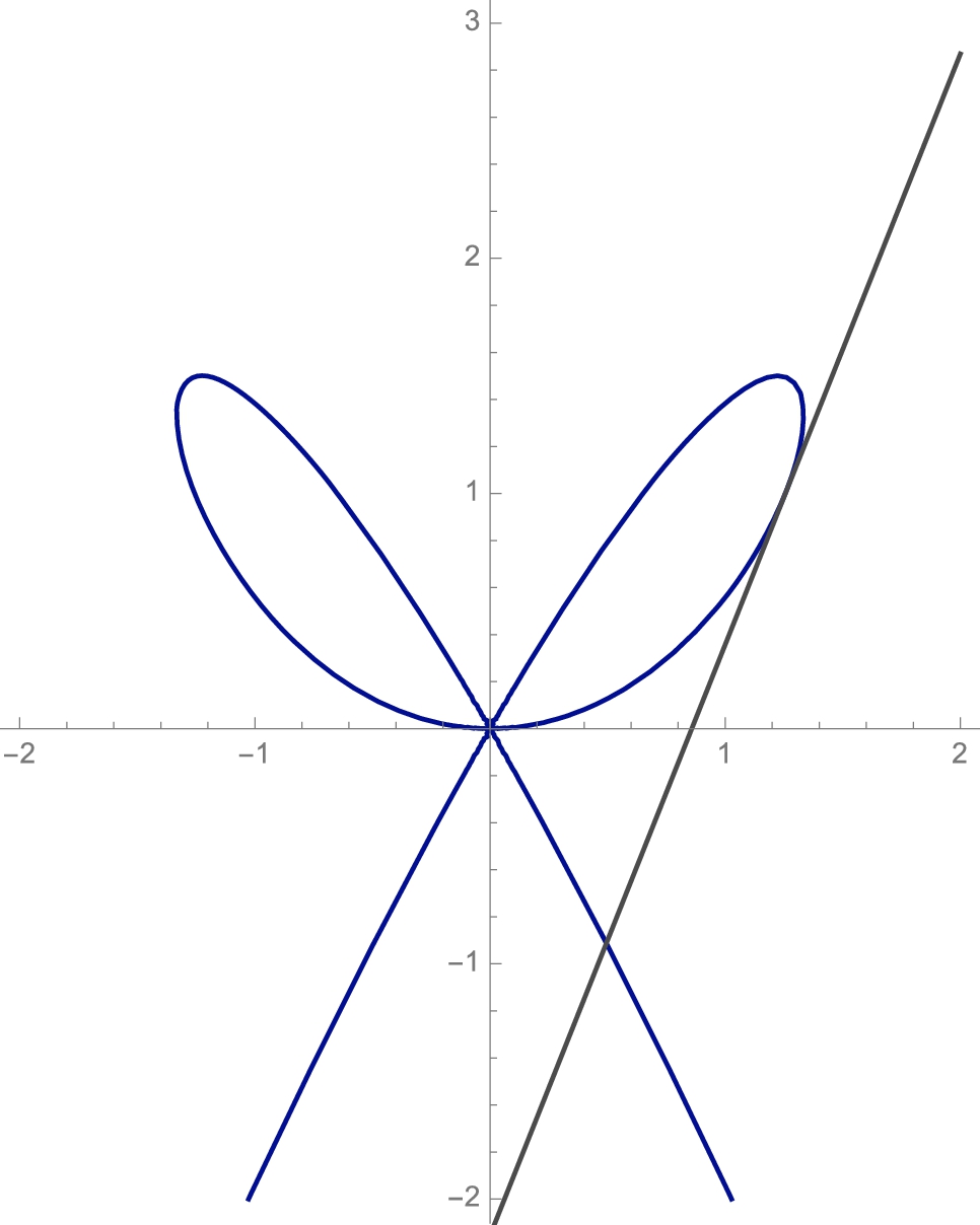
![]()
![]()
![]()
![]()
![]()
![]()
![]()
![]()
![]()
More generally, we use ContourPlot together with the StreamPlot function to illustrate that the gradient vectors are perpendicular to the level curves of ![]() in Fig. 3.67.
in Fig. 3.67.
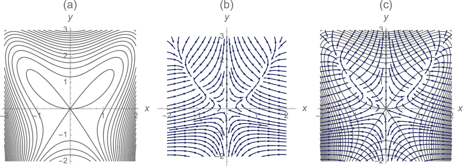
![]()
![]()
![]()
![]()
![]()
![]()
![]()
![]()
![]()
![]()
![]()
In Figs. 3.67 (b) and (c), observe that if the gradient vectors are all converging to a point, ![]() and the point will be a relative maximum. At
and the point will be a relative maximum. At ![]() ,
, ![]() but at this point, some gradient vectors are pointing towards the origin and some away so
but at this point, some gradient vectors are pointing towards the origin and some away so ![]() is a saddle. Compare to Fig. 3.65. Note that if
is a saddle. Compare to Fig. 3.65. Note that if ![]() and all the gradient vectors were pointing away from the point, the point would be a relative minimum. □
and all the gradient vectors were pointing away from the point, the point would be a relative minimum. □
Example 3.62
Solution
We begin by defining and graphing ![]() with Plot3D in Fig. 3.68 (a).
with Plot3D in Fig. 3.68 (a).
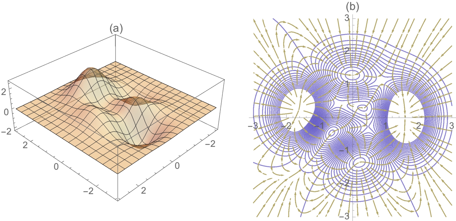
![]()
![]()
![]()
![]()
![]()
![]()
![]()
![]()
![]()
![]()
![]()
![]()
In the three-dimensional plot, notice that z appears to have six relative extrema: three relative maxima and three relative minima. We also graph several level curves of ![]() with ContourPlot and name the resulting graphic conf.
with ContourPlot and name the resulting graphic conf.
Next we calculate ![]() and
and ![]() using Simplify and D. The gradient is the vector-valued function
using Simplify and D. The gradient is the vector-valued function ![]() .
.
![]()
![]()
We use StreamPlot to graph the gradient naming the resulting graphic gradfplot. gradfplot and conf are displayed together using Show in Fig. 3.68 (b).
![]()
![]()
];
![]()
In the result (see Fig. 3.68 (b)), notice that the gradient is perpendicular to the level curves; the gradient is pointing in the direction of maximal increase of ![]() . □
. □
Classifying Critical Points
Let ![]() be a real-valued function of two variables with continuous second-order partial derivatives. A critical point of
be a real-valued function of two variables with continuous second-order partial derivatives. A critical point of ![]() is a point
is a point ![]() in the interior of the domain of
in the interior of the domain of ![]() for which
for which
or, equivalently, ![]() . Critical points are classified by the Second Derivatives (or Partials) test.
. Critical points are classified by the Second Derivatives (or Partials) test.
Theorem 3.18
Second Derivatives Test
Let ![]() be a critical point of a function
be a critical point of a function ![]() of two variables and let
of two variables and let
1. If ![]() and
and ![]() , then
, then ![]() has a relative (or local) minimum at
has a relative (or local) minimum at ![]() .
.
2. If ![]() and
and ![]() , then
, then ![]() has a relative (or local) maximum at
has a relative (or local) maximum at ![]() .
.
3. If ![]() , then
, then ![]() has a saddle point at
has a saddle point at ![]() .
.
4. If ![]() , no conclusion can be drawn and
, no conclusion can be drawn and ![]() is called a degenerate critical point.
is called a degenerate critical point.
Example 3.63
Find the relative maximum, relative minimum, and saddle points of ![]() .
.
Solution
After defining ![]() , the critical points are found with Solve and named critpts.
, the critical points are found with Solve and named critpts.
![]()
![]()
![]()
We then define dfxx. Given ![]() ,
, ![]() returns the ordered quadruple
returns the ordered quadruple ![]() ,
, ![]() , equation (3.36) evaluated at
, equation (3.36) evaluated at ![]() , and
, and ![]() .
.
![]()
![]()
![]()
![]()
For example,
![]()
![]()
shows us that a relative maximum occurs at ![]() . We then use /. (ReplaceAll) to substitute the values in each element of critpts into dfxx.
. We then use /. (ReplaceAll) to substitute the values in each element of critpts into dfxx.
![]()
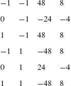
From the result, we see that ![]() results in a relative maximum,
results in a relative maximum, ![]() results in a saddle,
results in a saddle, ![]() results in a saddle,
results in a saddle, ![]() results in a relative minimum,
results in a relative minimum, ![]() results in a saddle, and
results in a saddle, and ![]() results in a relative minimum. We confirm these results graphically with a three-dimensional plot generated with Plot3D and a contour plot together with the gradient generated with ContourPlot and StreamPlot in Fig. 3.69.
results in a relative minimum. We confirm these results graphically with a three-dimensional plot generated with Plot3D and a contour plot together with the gradient generated with ContourPlot and StreamPlot in Fig. 3.69.

![]()
![]()
![]()
![]()
![]()
![]()
![]()
![]()
![]()
![]()
![]()
![]()
In the contour plot, notice that near relative extrema, the level curves look like circles while near saddles they look like hyperbolas. Further, at the maximums, the gradient is directed towards the point while at the minimums it is directed away from the point. □
If the Second Derivatives Test fails, graphical analysis is especially useful.
Example 3.64
Find the relative extrema and saddle points of ![]() .
.
Solution
Initially we proceed in the exact same manner as in the previous example: we define ![]() and compute the critical points. Several complex solutions are returned, which we ignore.
and compute the critical points. Several complex solutions are returned, which we ignore.
![]()
![]()
![]()
We then compute the value of (3.36) at the real critical point, and the value of ![]() at this critical point.
at this critical point.
![]()
![]()
![]()
![]()
![]()
![]()
The result shows us that the Second Derivatives Test fails at ![]() .
.
![]()
![]()
![]()
![]()
![]()
![]()
![]()
![]()
![]()
![]()
![]()
![]()
However, the contour plot and the stream plot of the gradient of ![]() near
near ![]() indicates that an extreme value occurs at
indicates that an extreme value occurs at ![]() . Because the gradient vectors are all pointing away from the origin,
. Because the gradient vectors are all pointing away from the origin, ![]() is a relative minimum which is confirmed in the three-dimensional plot. It is also an absolute minimum. (See Fig. 3.70.) □
is a relative minimum which is confirmed in the three-dimensional plot. It is also an absolute minimum. (See Fig. 3.70.) □
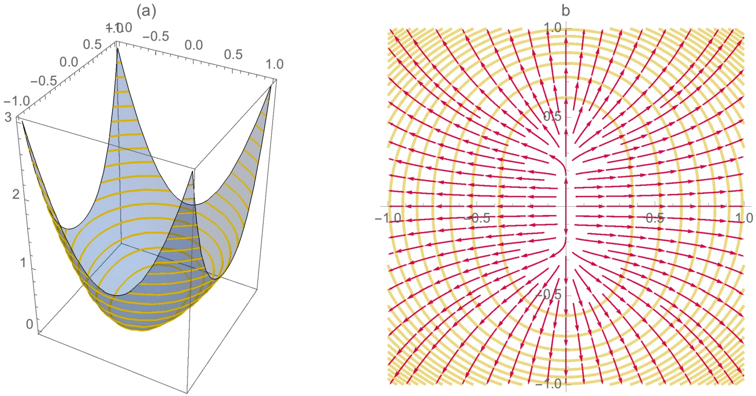
Tangent Planes
Let ![]() be a real-valued function of two variables. If both
be a real-valued function of two variables. If both ![]() and
and ![]() exist, then an equation of the plane tangent to the graph of
exist, then an equation of the plane tangent to the graph of ![]() at the point
at the point ![]() is given by
is given by
where ![]() . Solving for z yields the function (of two variables)
. Solving for z yields the function (of two variables)
Symmetric equations of the line perpendicular to the surface ![]() at the point
at the point ![]() are given by
are given by
and parametric equations are

The plane tangent to the graph of ![]() at the point
at the point ![]() is the “best” linear approximation of
is the “best” linear approximation of ![]() near
near ![]() in the same way as the line tangent to the graph of
in the same way as the line tangent to the graph of ![]() at the point
at the point ![]() is the “best” linear approximation of
is the “best” linear approximation of ![]() near
near ![]() .
.
Example 3.65
Find an equation of the plane tangent and normal line to the graph of ![]() at the point
at the point ![]() .
.
Solution
We define ![]() and compute
and compute ![]() and
and ![]() .
.
![]()
![]()
![]()
![]()
![]()
−1
−1
Using (3.38), an equation of the tangent plane is ![]() . Using (3.40), parametric equations of the normal line are
. Using (3.40), parametric equations of the normal line are ![]() ,
, ![]() ,
, ![]() . We confirm the result graphically by graphing
. We confirm the result graphically by graphing ![]() together with the tangent plane in p1 using Plot3D. We use ParametricPlot3D to graph the normal line in p2 and then display p1 and p2 together with Show in Fig. 3.71.
together with the tangent plane in p1 using Plot3D. We use ParametricPlot3D to graph the normal line in p2 and then display p1 and p2 together with Show in Fig. 3.71.
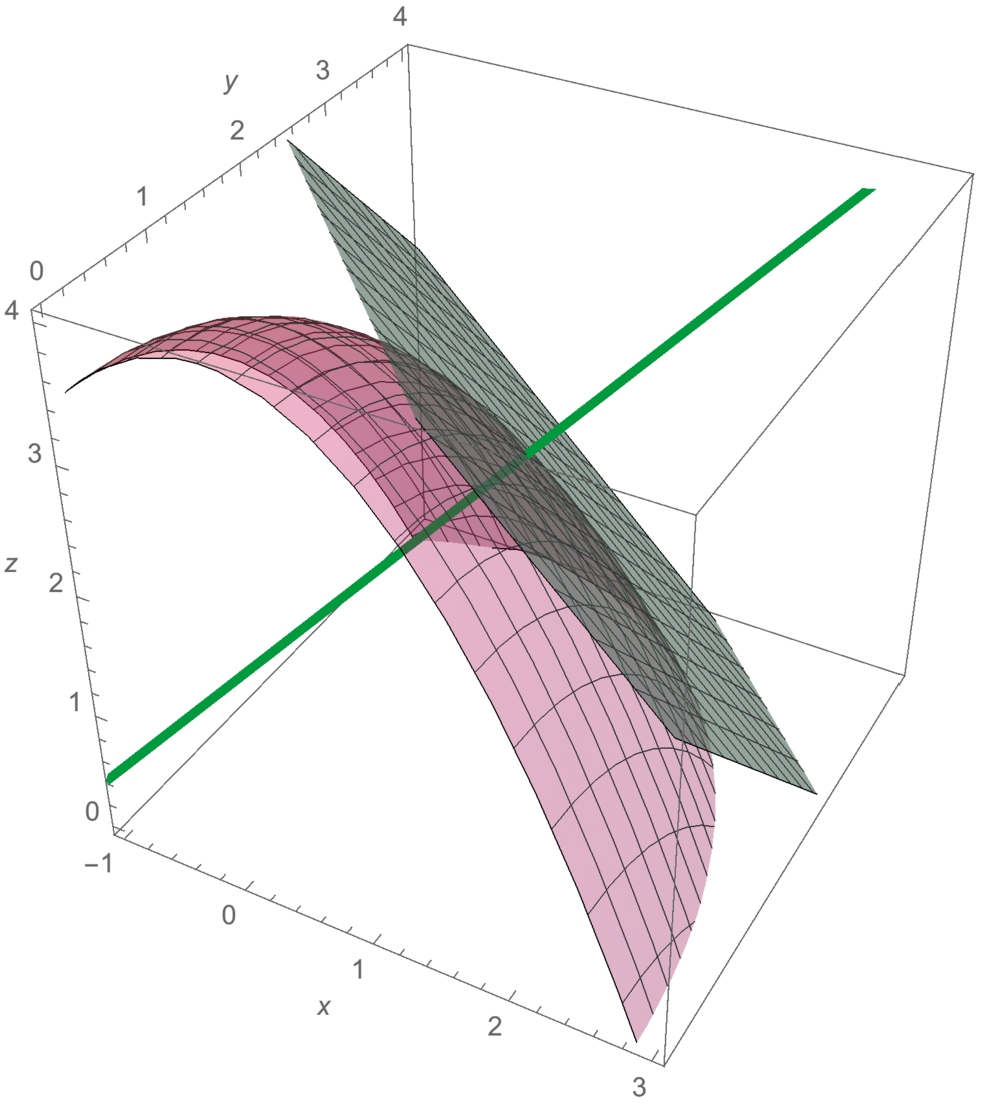
![]()
![]()
![]()
![]()
![]()
![]()
![]()
![]()
Because ![]() is the “best” linear approximation of
is the “best” linear approximation of ![]() near
near ![]() , the graphs are very similar near
, the graphs are very similar near ![]() as shown in the three-dimensional plot. We also expect the level curves of each near
as shown in the three-dimensional plot. We also expect the level curves of each near ![]() to be similar, which is confirmed with ContourPlot in Fig. 3.72.
to be similar, which is confirmed with ContourPlot in Fig. 3.72.
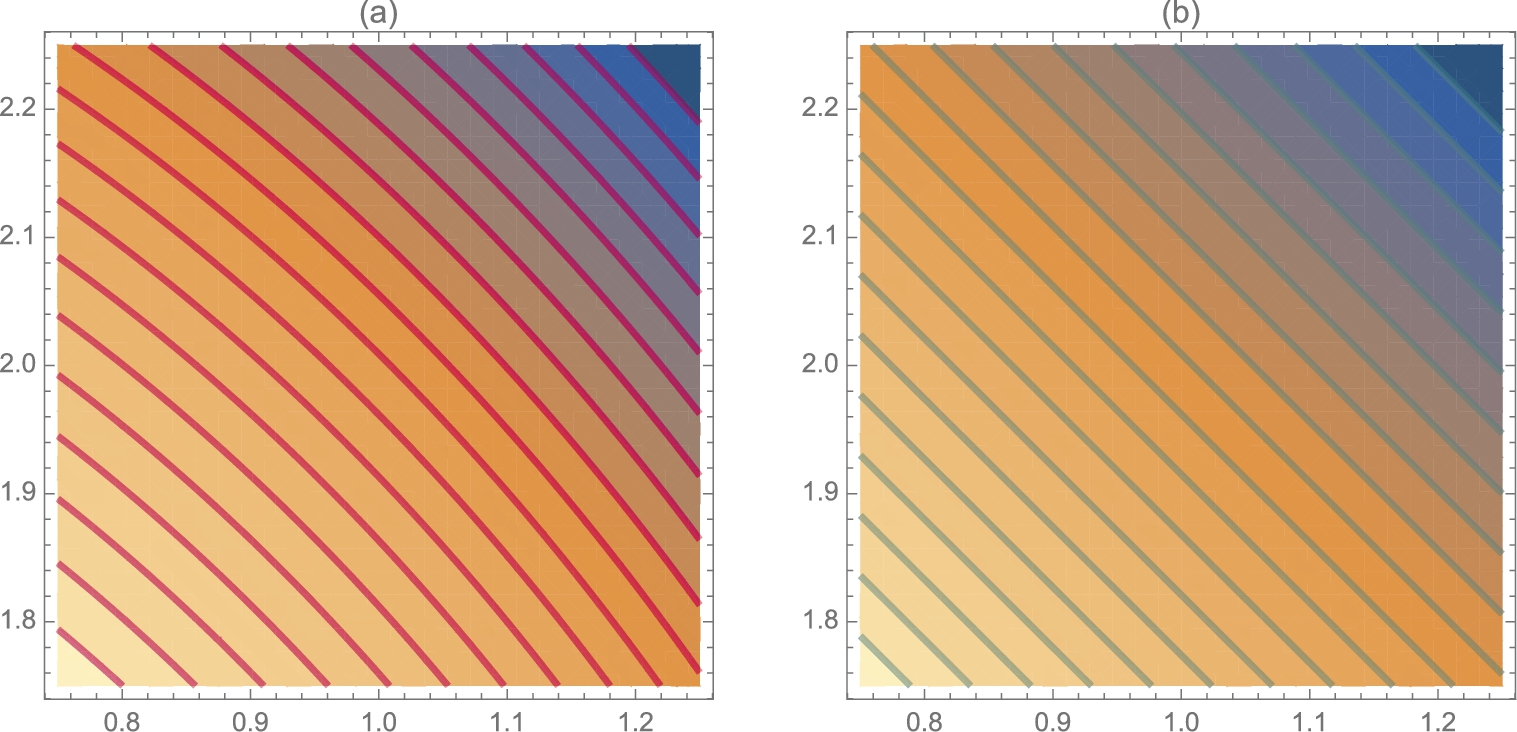
![]()
![]()
![]()
![]()
![]()
![]()
![]()
![]()
![]() □
□
Lagrange Multipliers
Certain types of optimization problems can be solved using the method of Lagrange multipliers that is based on the following theorem.
Theorem 3.19
Lagrange's Theorem
Graphically, the points ![]() at which the extreme values occur correspond to the points where the level curves of
at which the extreme values occur correspond to the points where the level curves of ![]() are tangent to the graph of
are tangent to the graph of ![]() .
.
Example 3.66
Find the maximum and minimum values of ![]() subject to the constraint
subject to the constraint ![]() .
.
Solution
For this problem, ![]() and
and ![]() . Observe that parametric equations for
. Observe that parametric equations for ![]() are
are ![]() ,
, ![]() ,
, ![]() . In Fig. 3.73 (a), we use ParametricPlot3D to parametrically graph
. In Fig. 3.73 (a), we use ParametricPlot3D to parametrically graph ![]() and
and ![]() for x and y-values on the curve
for x and y-values on the curve ![]() by graphing
by graphing
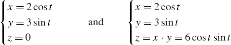
for ![]() . Our goal is to find the minimum and maximum values in Fig. 3.73 (a) and the points at which they occur.
. Our goal is to find the minimum and maximum values in Fig. 3.73 (a) and the points at which they occur.
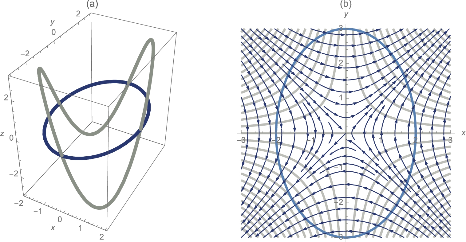
![]()
![]()
![]()
![]()
![]()
![]()
![]()
![]()
To implement the method of Lagrange multipliers, we compute ![]() ,
, ![]() ,
, ![]() , and
, and ![]() with D.
with D.
![]()
![]()
![]()
![]()
y
x
![]()
![]()
Solve is used to solve the system of equations (3.41):

for x, y, and λ.
![]()
![]()
The corresponding values of ![]() are found using ReplaceAll (/.).
are found using ReplaceAll (/.).
![]()
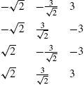
![]()
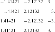
We conclude that the maximum value ![]() subject to the constraint
subject to the constraint ![]() is 3 and occurs at
is 3 and occurs at ![]() and
and ![]() . The minimum value is −3 and occurs at
. The minimum value is −3 and occurs at ![]() and
and ![]() . We graph several level curves of
. We graph several level curves of ![]() and the graph of
and the graph of ![]() with ContourPlot and show the graphs together with Show. The minimum and maximum values of
with ContourPlot and show the graphs together with Show. The minimum and maximum values of ![]() subject to the constraint
subject to the constraint ![]() occur at the points where the level curves of
occur at the points where the level curves of ![]() are tangent to the graph of
are tangent to the graph of ![]() as illustrated in Fig. 3.73 (b).
as illustrated in Fig. 3.73 (b).
![]()
![]()
![]()
![]()
![]()
![]()
![]()
![]()
![]()
![]()
![]()
Observe that the maximum and minimum values occur where the gradient vectors of ![]() are parallel to the gradient vectors of
are parallel to the gradient vectors of ![]() on the equation
on the equation ![]() . □
. □
3.5.3 Iterated Integrals
The Integrate command, used to compute single integrals, is used to compute iterated integrals. The command
Integrate[f[x,y],{y,c,d},{x,a,b}]
attempts to compute the iterated integral
If Mathematica cannot compute the exact value of the integral, it is returned unevaluated, in which case numerical results may be more useful. The iterated integral (3.42) is numerically evaluated with the command N or
NIntegrate[f[x,y],{y,c,d},{x,a,b}]
Example 3.67
Evaluate each integral: (a) ![]() ; (b)
; (b) ![]() ; (c)
; (c) ![]() ; (d)
; (d) ![]() .
.
Solution
(a) First, we compute ![]() with Integrate. Second, we compute
with Integrate. Second, we compute ![]() with Integrate.
with Integrate.
![]()
![]()
![]()
98
(b) We illustrate the same commands as in (a), except we are integrating over a nonrectangular region.
![]()
![]()
![]()
![]()
![]()
![]()
(c) Improper integrals can be handled in the same way as proper integrals.
![]()
![]()
![]()
![]()
(d) In this case, Mathematica cannot evaluate the integral exactly so we use NIntegrate to obtain an approximation.
![]()
![]()
![]()
15.5092 □
Area, Volume, and Surface Area
Typical applications of iterated integrals include determining the area of a planar region, the volume of a region in three-dimensional space, or the surface area of a region in three-dimensional space. The area of the planar region R is given by
If ![]() has continuous partial derivatives on a closed region R, then the surface area of the portion of the surface that projects onto R is given by
has continuous partial derivatives on a closed region R, then the surface area of the portion of the surface that projects onto R is given by

If ![]() on R, the volume of the region between the graphs of
on R, the volume of the region between the graphs of ![]() and
and ![]() is
is

Example 3.68
Find the area of the region R bounded by the graphs of ![]() and
and ![]() .
.
Solution
We begin by graphing ![]() and
and ![]() with Plot in Fig. 3.74. The x-coordinates of the intersection points are found with Solve.
with Plot in Fig. 3.74. The x-coordinates of the intersection points are found with Solve.
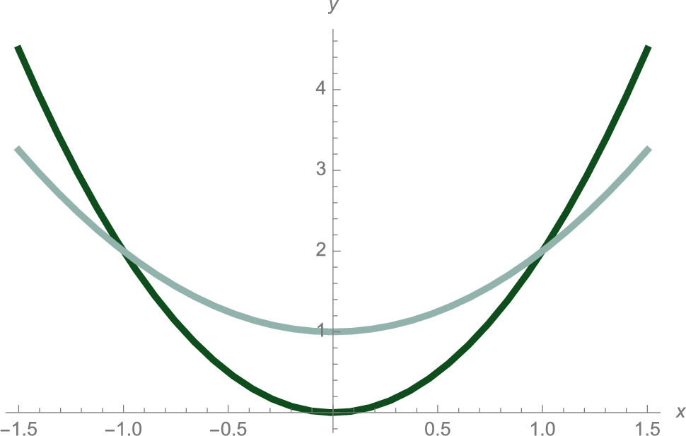
![]()
![]()
![]()
![]()
![]()
![]()
Using (3.43) and taking advantage of symmetry, the area of R is given by
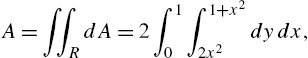
which we compute with Integrate.
![]()
![]()
We conclude that the area of R is 4/3. □
If the problem exhibits “circular symmetry,” changing to polar coordinates is often useful. If ![]() , then
, then
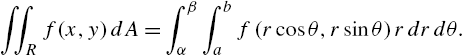
Example 3.69
Solution
First, observe that the domain of ![]() is
is

Similarly,

With this observation, we use ParametricPlot3D to graph ![]() in p1 and the portion of the graph of
in p1 and the portion of the graph of ![]() above R in p2 and show the two graphs together with Show. We wish to find the area of the black region in Fig. 3.75.
above R in p2 and show the two graphs together with Show. We wish to find the area of the black region in Fig. 3.75.
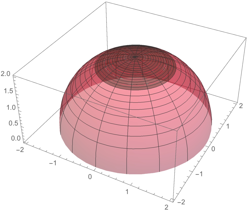
![]()
![]()
![]()
![]()
![]()
![]()
![]()
![]()
We compute ![]() ,
, ![]() and
and ![]() with D and Simplify.
with D and Simplify.
![]()
![]()
![]()
![]()
![]()
![]()
Then, using (3.44), the surface area is given by
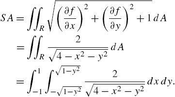
However, notice that in polar coordinates,
so in polar coordinates the surface area is given by

![]()
![]()
which is much easier to evaluate than (3.46). We evaluate the iterated integral with Integrate
![]()
![]()
![]()
3.36715
and conclude that the surface area is ![]() . □
. □
Example 3.70
Find the volume of the region between the graphs of ![]() and
and ![]() .
.
Solution
We begin by graphing ![]() and
and ![]() together with Plot3D in Fig. 3.76 (a). The region of integration, R, is determined by graphing
together with Plot3D in Fig. 3.76 (a). The region of integration, R, is determined by graphing ![]() with ContourPlot in Fig. 3.76 (b).
with ContourPlot in Fig. 3.76 (b).
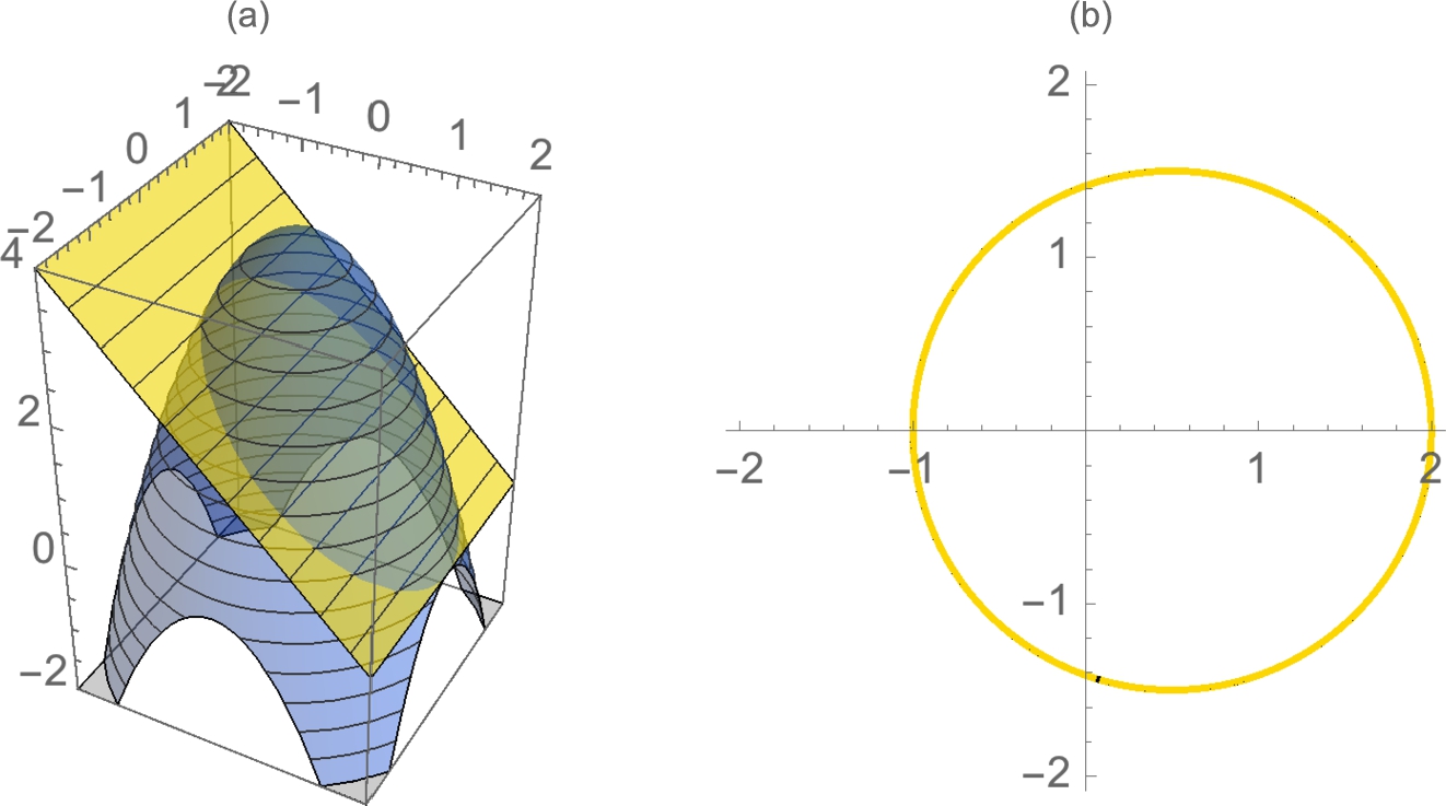
![]()
![]()
![]()
![]()
![]()
![]()
![]()
![]()
![]()
![]()
Another way to see the situation illustrated in Fig. 3.77 is to use RegionPlot3D, which works in the same way as RegionPlot but in three dimensions.
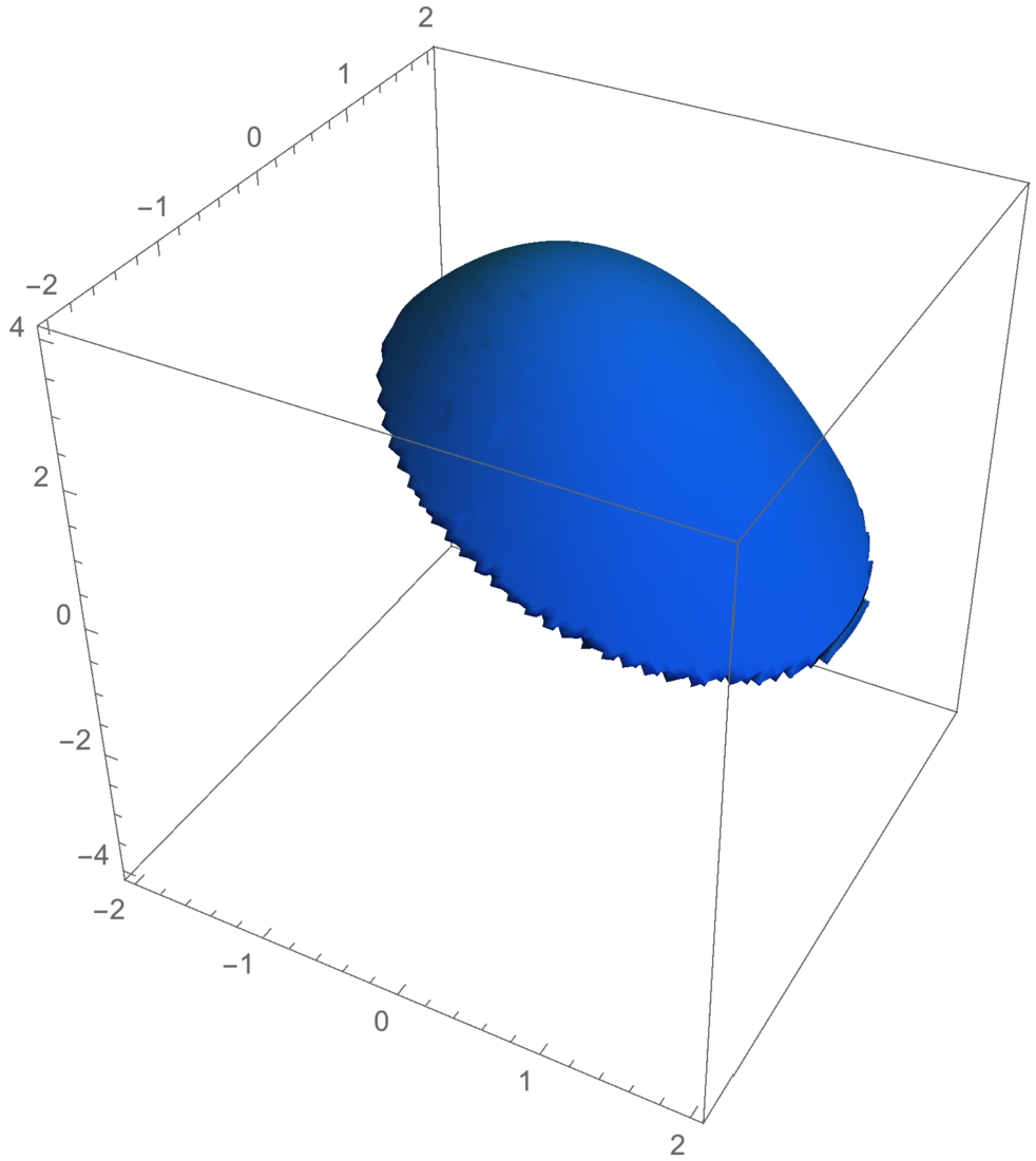
![]()
![]()
![]()
Completing the square shows us that
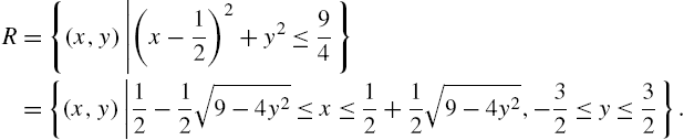
Thus, using (3.45), the volume of the solid is given by
which we evaluate with Integrate.
![]()
![]()
![]()
![]()
7.95216
We conclude that the volume is ![]() . □
. □
Triple Iterated Integrals
Triple iterated integrals are calculated in the same manner as double iterated integrals.
Solution
Entering
![]()
![]()
calculates the triple integral exactly with Integrate.
An approximation of the exact value is found with N.
![]()
0.157206 □
We illustrate how triple integrals can be used to find the volume of a solid when using spherical coordinates.
Example 3.72
Find the volume of the torus with equation in spherical coordinates ![]() .
.
Solution
We proceed by graphing the torus with SphericalPlot3D in Fig. 3.79 (see Fig. 3.78 for the help feature associated with this command).
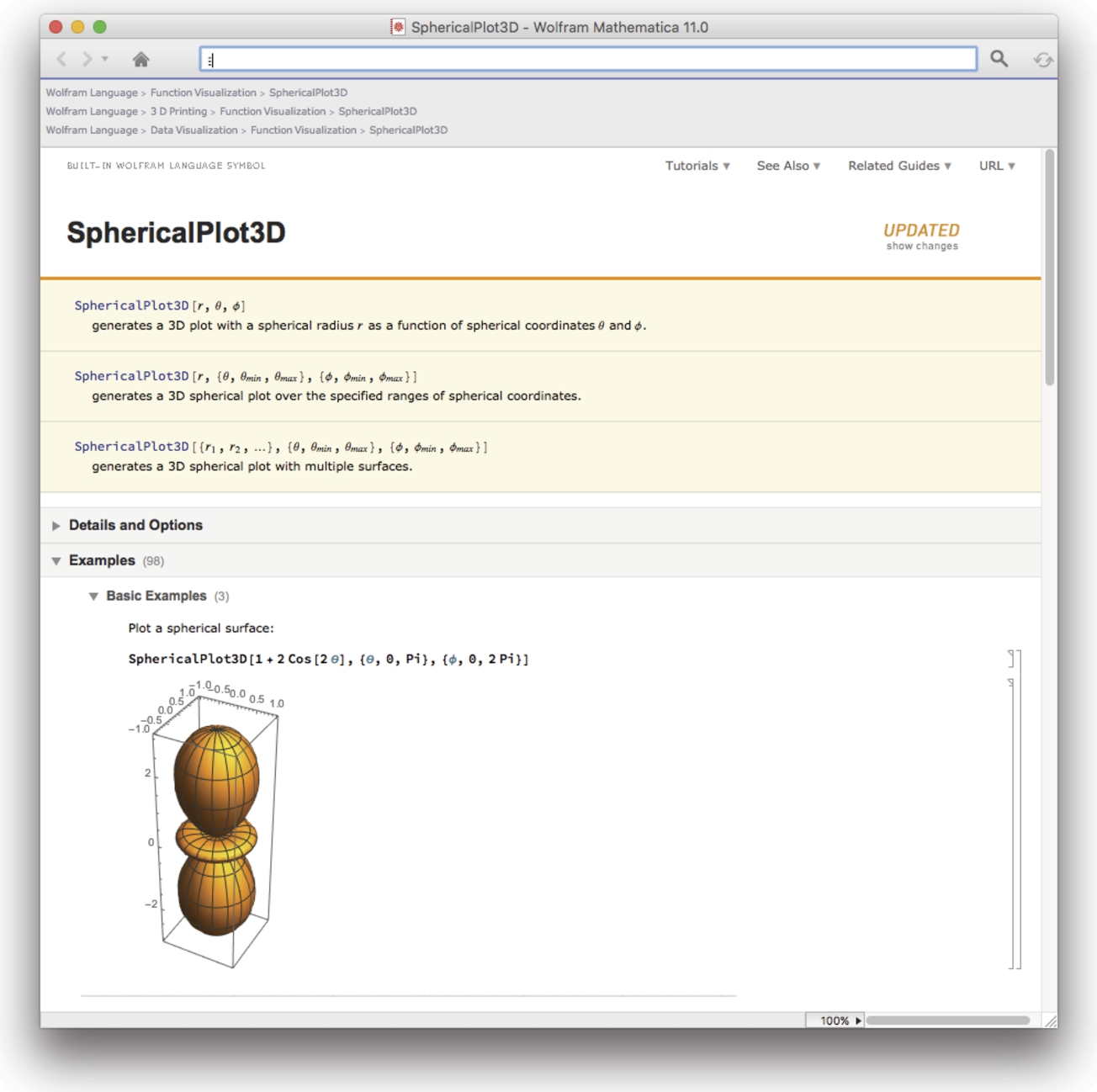
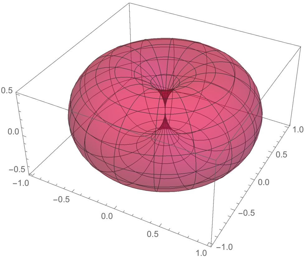
![]()
In general, the volume of the solid region D is given by
Thus, the volume of the torus is given by the triple iterated integral
![]()
![]()
![]()
![]()
2.4674
which we evaluate with Integrate. We conclude that the volume of the torus is ![]() . □
. □