Chapter 19: Summarizing Data with SAS Procedures

Introduction

This chapter describes how to summarize numeric data (means, standard deviations, etc.), and how to create SAS data sets containing this summary information. The main tools are PROC MEANS, PROC SUMMARY, and PROC UNIVARIATE.

Using PROC MEANS (with the Default Options)

PROC MEANS is one of the most useful procedures for summarizing data. As you will see in the programs that follow, you can run this procedure without specifying any options and obtain useful information, including the number of nonmissing observations, the mean, the standard deviation, and the minimum and the maximum values for all the numeric variables in the data set. Later on, in this chapter, you will see how to add procedure options and statements to customize the summary report.

To demonstrate the various ways that you can use PROC MEANS to summarize data, run Program 19.1 to create a data set called Blood_Pressure. The program uses a random number generator to create a data set containing data from a fictitious drug trial.

The details of how this program works are not described in detail here, but some general information about this program might be interesting. First, remember that the library Oscar was created in a statement that you added to the Autoexec.sas file. The RAND function is used to generate random numbers that are normally distributed. The way the program is designed, if you run it yourself, you will obtain exactly the same data set used in the examples that follow. The program also generates a subject number, drug group, and gender, as well as the systolic and diastolic blood pressure (adjusted so that the drug group pressures are lower than the placebo group pressures). The program also outputs missing values for some of the variables, to make the data set more realistic. Here is the program.

Program 19.1: Creating the Blood_Pressure Data Set

Libname Oscar “~/MyBookFiles”;
/* Not necessary if already in your Autoexec.sas file */

data Oscar.Blood_Pressure;
   call streaminit(37373);
   do Drug = ‘Placebo’,’Drug A’,’Drug B’;
      do i = 1 to 20;
         Subj + 1;
         if mod(Subj,2) then Gender = ‘M’;
         else Gender = ‘F’;
         SBP = rand(‘normal’,130,10) +
               7*(Drug eq ‘Placebo’) - 6*(Drug eq ‘Drug B’);
         SBP = round(SBP,2);
         DBP = rand(‘normal’,80,5) +
               3*(Drug eq ‘Placebo’) - 2*(Drug eq ‘Drug B’);
         DBP = round(DBP,2);
         Age = int(rand(‘normal’,50,10) + .1*SBP);         
         if Subj in (5,15,25,55) then call missing(SBP, DBP);
         if Subj in (4,18) then call missing(Gender);
         output;
      end;
   end;
   drop i;
run;

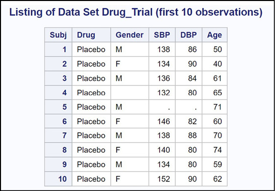
title “Listing of Data Set Drug_Trial (first 10 observations)”;
proc print data=Oscar.Blood_Pressure(obs=10);
   id Subj;
run;

The first 10 observations of this data set are listed next.

Figure 19.1: Output from Program 19.1

You are now ready to run PROC MEANS (without specifying any options) on this data set.

Program 19.2: Running PROC MEANS on the Blood_Pressure Data Set (Using All the Default Options)

title “Running PROC MEANS with all the Defaults”;
proc means data=Oscar.Blood_Pressure;
run;

After running this program, the RESULTS window looks like this:

Figure 19.2: Output from Program 19.2

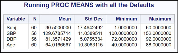
Because you did not include a VAR statement, PROC MEANS summarized every numeric variable in the Blood_Pressure data set (including the subject number). Let’s see how to produce a more meaningful report.

Using PROC MEANS Options to Customize the Summary Report

Most of the time, you will want to override the default output and select the statistics that you want in your report. The following table shows some of the most popular statistics that you can request using PROC MEANS:

Table 19.1: Table of PROC MEANS Options

Option	Description
N	The number of nonmissing observations used to compute the statistics
NMISS	The number of missing observations
MEAN	The mean
STD	The standard deviation
CV	The coefficient of variation
CLM	The 95% confidence interval for the mean
STDERR	The standard error
MIN	The minimum value
MAX	The maximum value
MEDIAN	The median
MAXDEC=n	The maximum number of decimal places in all the table values

You will probably want to include the MAXDEC= option every time you run PROC MEANS, whether you override the default options or not. This option controls the number of digits to the right of the decimal place for most of the statistics in the output (values for N and NMISS are always integers).

In most cases, you will also want to use the N and NMISS options. These two options add the number of nonmissing and missing values in the output table.

What other options you select will vary depending on what information you need for your particular project. The next program uses MAXDEC, N, and NMISS along with options to print the mean, the standard deviation, the coefficient of variation, the standard error, and the 95% confidence interval for the mean. These statistics are commonly used in reports and journal articles. Here is the program, followed by the output.

Program 19.3: Adding Options to Control PROC MEANS Output

title “Running PROC MEANS with Selected Options”;
proc means data=Oscar.Blood_Pressure n nmiss mean std cv stderr clm    maxdec=3;
   var SBP DBP;
run;

A VAR statement was also included in this program to request statistics only for the two variables SBP and DBP (systolic and diastolic blood pressure).

Most of the time, you will want to include a VAR statement when you use PROC MEANS because there might be several numeric variables in your data set for which it makes no sense to compute means and other statistics (such as the subject variable in this data set).

Here is the output.

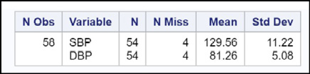
Figure 19.3: Output from Program 19.3

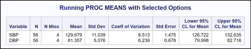
Once you specify any PROC MEANS options (with the exception of MAXDEC=), the output will contain statistics only for the options that you specify. Notice that the minimum and maximum values, part of the default set of statistics, are not present in this output.

This summary table displays statistics for SBP and DBP for all subjects in the trial. The next step is to see a breakdown of these statistics by Gender and Drug.

Computing Statistics for Each Value of a BY Variable

It is often useful to compute statistics for each value of some other variable. For example, one of the variables in the Blood_Pressure data set is Gender. You might want to see selected statistics for males and females. One way to do this is to sort the data set by Gender and then include a BY statement with PROC MEANS.

The next program does just this.

Program 19.4: Adding a BY Statement with PROC MEANS

proc sort data=Oscar.Blood_Pressure out=Blood_Pressure;
   by Gender;
run;

title “Statistics for Blood Pressure Study Broken Down by Gender”;
proc means data=Blood_Pressure n nmiss mean std maxdec=2;
   by Gender;
   var SBP DBP;
run;

You add an OUT= PROC SORT option so that the data in the original (permanent) data set is not affected. You can use the same data set name (Blood_Pressure) for the output data set in the Work library as you used in the permanent library.

Most of the time, when you run PROC SORT, you should specify an OUT= procedure option, especially if you are subsetting either observations or variables. This prevents you from damaging the original data set.

Because you added the BY statement to PROC MEANS, you now have your statistics broken down by Gender. Here is a portion of the output.

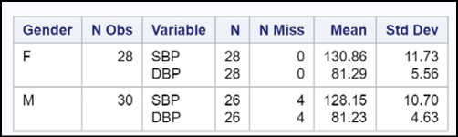
Figure 19.4: Output from Program 19.4

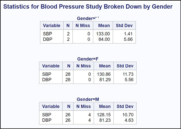
You now see the N, NMISS, mean, and standard deviation for males and females (as well as the two observations where Gender was missing).

If you want to omit the two observations where Gender is missing, add a WHERE= data set option as part of your PROC SORT, like this:

proc sort data=Oscar.Blood_Pressure(where=(Gender is not missing)) 

   out=Blood_Pressure;

The output data set, Blood_Pressure, is now sorted by Gender and does not include any observations with missing values for Gender. This also shows why it is usually advantageous to include an OUT= option with PROC SORT. Without it, you would have removed two observations from your permanent Blood_Pressure data set.

Using a CLASS Statement Instead of a BY Statement

You can use a CLASS statement to generate the same information that you produced with a BY statement. One major difference between using a BY statement versus a CLASS statement is that you do not have to sort the data when you use a CLASS statement.

If you have very large data sets and several CLASS variables, there is a possibility that the program will run out of memory, and you will have to use PROC SORT and a BY statement instead of a CLASS statement. Using cloud based programs, this situation is highly unlikely.

The output that you obtain when you use a CLASS statement instead of a BY statement has a slightly different, more compact format, but the numbers are the same. The next program shows how to use a CLASS statement:

Program 19.5: Using a CLASS Statement to See Statistics Broken Down by Region

title “Using a CLASS Statement with PROC MEANS”;
proc means data=Oscar.Blood_Pressure n nmiss mean std maxdec=2;
   class Gender;
   var SBP DBP;
run;

Notice that this program is using the original permanent data set and no sorting is necessary. Here is the result:

Figure 19.5: Output from Program 19.5

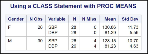
Using a CLASS statement produces a slightly more compact and easy-to-read report. Also, it does not include the observations where Gender is missing.

Including Multiple CLASS Variables with PROC MEANS

Because this was a drug study, you will want to see statistics on SBP and DBP broken down by Gender and Drug. This is easily accomplished by listing these two variables in the CLASS statement. Here is the program and the output.

Program 19.6: Using Two CLASS Variables with PROC MEANS

title “Using a CLASS Statement with Two CLASS Variables”;
proc means data=Oscar.Blood_Pressure n nmiss mean std maxdec=2;
   class Gender Drug;
   var SBP DBP;
run;

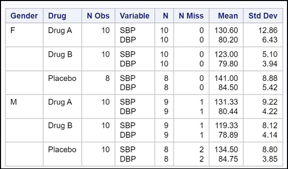
Figure 19.6: Output from Program 19.6

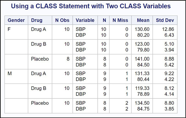
You now see blood pressures broken down by Gender and Drug.

Statistics Broken Down Every Way

You can add the PROC MEANS option PRINTALLTYPES to output statistics broken down by every combination of the CLASS variables. To show how this works, here is Program 19.6 rewritten with this option included.

Program 19.7: Adding the PRINTALLTYPES Option to PROC MEANS

proc means data=Oscar.Blood_Pressure n nmiss mean std maxdec=2
   printalltypes;
   class Gender Drug;
   var SBP DBP;
run;

The output now looks like this.

Figure 19.7: Output from Program 19.7

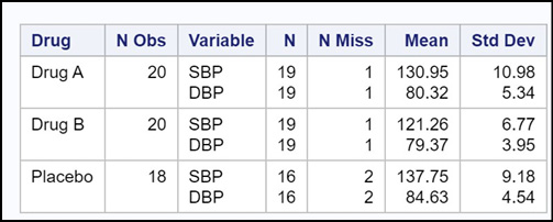
You now see statistics for every combination of the CLASS variables. This is a very useful option and you should always consider using it when you have one or more CLASS variables.

Using PROC MEANS to Create a Summary Data Set

Besides producing printed output, you can use PROC MEANS to create a data set containing the same data that was in the printed reports. Let’s start out by computing the mean SBP and DBP for the entire data set. To do this, you add an OUTPUT statement. On this statement, you name the output data set and specify what statistics you want in that data set. For this first example, you will name the data set Grand_Mean and request that the mean and the number of nonmissing observations be included in the data set. Here is the program.

Program 19.8: Using PROC MEANS to Create a Data Set Containing the Grand Mean

proc means data=Oscar.Blood_Pressure noprint;
   var SBP DBP;
   output out=Grand_Mean mean=Grand_SBP Grand_DBP 
          n=Nonmiss_SBP Nonmiss_DBP;   
run;

Because you want to create a summary data set and do not want to print a report, you use the PROC MEANS option NOPRINT. This option suppresses any printed output from the procedure.

PROC SUMMARY produces data sets identical to those produced by PROC MEANS. The only difference between the two procedures is that PROC SUMMARY automatically includes a NOPRINT option. So, use PROC MEANS with the NOPRINT option or PROC SUMMARY—your choice.

You use an OUTPUT statement where you specify the name of the output data set (with the keyword OUT=), and you use keywords to specify which statistics you want in the output data set. These keywords are the same ones that you used as PROC MEANS options (see the keywords for PROC MEANS earlier in this chapter) followed by an equal sign, followed by the variable names that you want to use. These variable names are in the same order as the variable names on the VAR statement. The variable Grand_SBP is the mean SBP for all observations in the data set; the variable Grand_DBP is the mean DBP for all observations in the data set.

Even if you are an experienced SAS programmer, it is a good idea to use PROC PRINT to list the contents of the summary data set. Program 19.9 does this.

Program 19.9: Listing of Data Set Grand_Mean

title “Listing of Data Set Grand_Mean”;
proc print data=Grand_Mean noobs;
run;

Here is the listing.

Figure 19.8: Output from Program 19.9

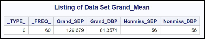
This data set contains the four variables that you specified in the OUTPUT statement (two for SBP and two for DBP). SAS has added two additional variables to this data set: _TYPE_ and _FREQ_. The variable _TYPE_ is useful when you have one or more CLASS variables. The variable _FREQ_ is the total number of observations available for use in the data set. There were 60 observations in data set Blood_Pressure, but because there were four missing values for SBP and DBP, both variables Nonmiss_SBP and Nonmiss_DBP are equal to 56.

Letting PROC MEANS Name the Variables in the Output Data Set

A nice option that you can use with an OUTPUT statement is called AUTONAME. When you include this option, you do not have to name any of the variables in the output data set—PROC MEANS will name them for you. It uses the names on the VAR statement and adds an underscore, followed by the statistic that you requested. For example, if you want the mean for SBP and DBP, the output data set will use the variable names SBP_Mean and DBP_Mean. Here is Program 19.8 rewritten to use the AUTONAME option.

Program 19.10: Using AUTONAME to Name the Variables in the Output Data Set

proc means data=Oscar.Blood_Pressure noprint;
   var SBP DBP;
   output out=Grand_Mean mean= n= / autoname;   
run;

title “Listing of Data Set Grand_Mean”;
title2 “Using the AUTONAME Output Option”;
proc print data=Grand_Mean noobs;
run;

You use the keywords for the desired statistics, followed by an equal sign and no variable names. Because AUTONAME is a statement option, it follows a slash in the OUTPUT statement. Here is a listing of data set Grand_Mean where the AUTONAME option was used.

Figure 19.9: Output from Program 19.10

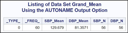
This author recommends using AUTONAME for two reasons: One, it saves entering and creating variable names for all your statistics; and two, it creates consistent and predictable variable names for all of your statistics.

Creating a Summary Data Set with CLASS Variables

You might want to create a summary data set that contains statistics broken down by one or more variables. One way to do this is to add a CLASS statement to PROC MEANS, along with an OUTPUT statement. This produces an especially useful data set. To demonstrate this process, let’s output several statistics for the variables SBP and DBP and include both Gender and Drug as CLASS variables. Here is the program.

Program 19.11: Creating a Summary Data Set with Two CLASS Variables

proc means data=Oscar.Blood_Pressure noprint;
   class Gender Drug;
   var SBP DBP;
   output out=Summary mean= n= std= / autoname;
run;

title “Listing of Data Set Summary”;
proc print data=Summary noobs;
run;

You are requesting values for the mean, the number of nonmissing values, and the standard deviation for the variables SBP and DBP, broken down by Gender and Drug. Here is a listing of the data set.

Figure 19.10: Output from Program 19.11

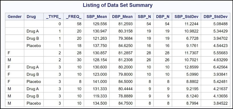
This might not be what you expected. The first observation (_TYPE_ = 0) is the mean (along with the other requested statistics) for all the observations. The next three observations are statistics broken down by Drug; the next two observations are statistics broken down by Gender; and, finally, the last six observations show the statistics for every combination of Drug and Gender. Notice that the suffix added for the two variables holding the standard deviations is StdDev, not Std (the option that you used). The reason is that Std is an abbreviation for the actual term StdDev.

You probably want only the last six observations in this data set. The easiest way to do this is to add the PROC MEANS option NWAY. This option provides your requested statistics broken down by all of your CLASS variables. Here is Program 19.11 rewritten to include the NWAY option.

Program 19.12: Adding the NWAY Option to PROC MEANS

proc means data=Oscar.Blood_Pressure noprint nway;
   class Gender Drug;
   var SBP DBP;
   output out=Summary mean= n= std= / autoname;
run;

title “Listing of Data Set Summary”;
title2 “NWAY Option Added”;
proc print data=Summary noobs;
run;

Here is the listing of the Summary data set.

Figure 19.11: Output from Program 19.12

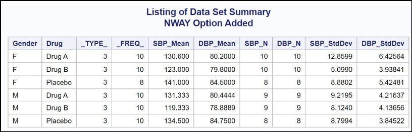
You now have the data set you want.

If you sorted the Blood_Pressure data set by Gender and Drug and used a BY statement instead of a CLASS statement, you would not need the NWAY option. The data set would be identical to the one above.

It is very important to remember the NWAY option when all you want are the statistics broken down by all of the CLASS variables. This author uses the mental “trick” of pairing NOPRINT and NWAY together in his mind.

Using a Formatted CLASS Variable

The Blood_Pressure data set also contains the age of each subject in the study. You might want to see the mean systolic and diastolic blood pressures for two or more age groups. Conveniently, if you use a continuous variable such as Age in a CLASS statement and you also include a FORMAT statement, PROC MEANS will use the formatted values of the CLASS variables to compute statistics. Here is an example:

You want to see the mean and standard deviation of SBP and DBP for three age groups:

● Low–50

● 51–70

● 71–High

All you need to do is create a format and include CLASS and FORMAT statements when you run PROC MEANS. The next program demonstrates this.

Program 19.13: Using a Formatted CLASS Variable

proc format;
   value AgeGroup low-50  = ‘50 and Lower’
                   51-70   = ‘51 to 70’
                   71-high = ‘71 +’;
run;

title “Using a Formatted CLASS Variable”;
proc means data=Oscar.Blood_Pressure n nmiss mean std maxdec=2;
   class Age;
   format Age AgeGroup.;
   var SBP DBP;
run;

Here is the output.

Figure 19.12: Output from Program 19.13

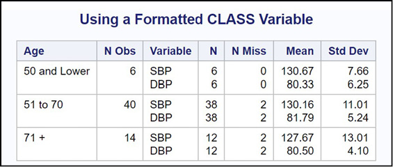
Using formatted CLASS variables enables you to see all of your statistics broken down by any grouping of continuous variables. It saves time and effort.

Demonstrating PROC UNIVARIATE

One of the most popular procedures for summarizing data, especially for statistical purposes, is PROC UNIVARIATE. This procedure has a lot in common with PROC MEANS. However, you can use statements to produce histograms and probability plots that are not available with PROC MEANS.

To demonstrate this procedure, the next program uses PROC UNIVARIATE to analyze SBP and produce a histogram and Q-Q plot.

Program 19.14: Demonstrating PROC UNIVARIATE

title “Demonstrating PROC UNIVARIATE”;
proc univariate data=Oscar.Blood_Pressure;
   id Subj;
   var SBP;
   histogram;
   qqplot / normal (mu=est sigma=est);
run;

If you have a variable such as Subj or ID, be sure to include an ID statement including that variable. It will be useful in some of the output. You use a VAR statement just as you did with PROC MEANS. Two additional statements, HISTOGRAM and QQPLOT, were added. HISTOGRAM, as the name implies, generates a histogram for all the variables on the VAR statement. QQPLOT requests a quantile-quantile plot, that is used by statisticians to help determine deviations from normality. When you request a Q-Q plot, you can add the option NORMAL. This option draws a straight line representing what a normal distribution would look like on the plot. Following this option, you can specify a mean (mu) and a standard deviation (sigma) for your theoretical normal plot. In this example, you want to use the data to estimate these two values. You use the term EST (stands for estimated) to request this.

Here is the result.

Figure 19.13: Output from Program 19.14

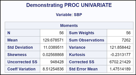
This first section shows you the mean, the standard deviation, and several other statistics. For those who are interested, the skewness and kurtosis are values that help determine whether the data values are normally distributed. For both of these statistics, values close to 0 indicate a distribution close to normal.

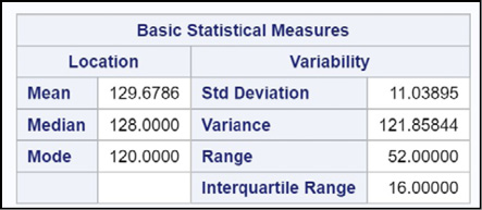
Here you see other measures of central tendency, including the mean and median, along with measures of spread or dispersion.

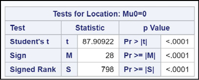
Here you see statistical tests to test the null hypothesis that the mean is 0.

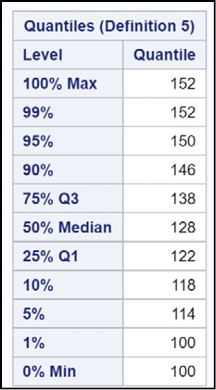
This section of output shows values of your variable at several different quantiles. In this section, you see that the largest value for SBP was 152 and the lowest was 100. The 25th percentile and the 75th percentile (122 and 138, respectively) are also popular measures.

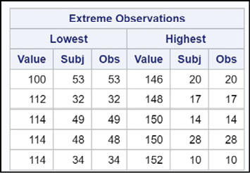
The section shows the five lowest and five highest observations in the data set. The section is especially useful to check if you have some extreme values, possibly data errors. You can have PROC UNIVARIATE print out more than five extreme observations by using a procedure option called NEXTROBS=N, where N is the number of high and low values that you want listed in the table. NEXTROBS stands for Number of EXTReme OBServations.

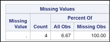
Here you see the number of missing values as a count and also as a percentage of all observations (6.67% in this data set).

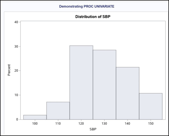
This histogram was produced by the HISTOGRAM statement. If you want to change the bin sizes, you can use a MIDPOINTS= option in the HISTOGRAM statement. For example, to see bars from 100 to 150 but with a bin width of 5 instead of 10, the HISTOGRAM statement would look like this:

histogram / midpoints=100 to 150 by 5;

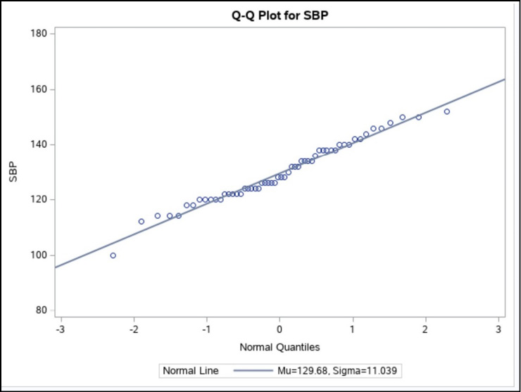
Finally, this is the Q-Q plot. You can see that the data points fall along a straight line, indicating that the values of SBP are close to normally distributed. If you prefer, you can substitute PROBPLOT for QQPLOT to obtain a similar plot called a probability plot.

Conclusion

This chapter covered a lot of ground. Besides showing you how to generate summary statistics, you saw how to use PROC MEANS to create a data set containing summary information. This process blurs the distinction between DATA steps and PROC steps. You now know how to create a data set by running a procedure.

There are some topics that were not covered in detail. For example, there are ways to use and interpret the _TYPE_ variable placed in the output data set by PROC MEANS. At some point, you might also want to combine the summary data generated by PROC MEANS with the original raw data. For more information about these topics, I recommend the following book:

Cody, Ron. 2011. SAS Statistics by Example. Cary, NC: SAS Institute Inc.

Problems

1. Starting with the SASHELP data set Heart, compute the following statistics for Height and Weight:

1. Number of nonmissing values

2. Number of missing values

3. Mean

4. Standard deviation

5. Minimum

6. Maximum

Use the appropriate option to print statistics 3 through 6 with two places to the right of the decimal point.

2. Repeat Problem 1 except use a BY statement to compute the statistics broken down by Status.

3. Repeat Problem 2 except use a CLASS statement instead of a BY statement.

4. Repeat Problem 3 except use the two CLASS variables Sex and Status. In addition, use the procedure option to show the statistics broken down by every one of the CLASS variables.

5. Repeat Problem 1 except produce an output data set (Summary) instead of printed output. Use the AUTONAME option in the OUTPUT statement to name all of the variables in the Summary data set.

6. Repeat Problem 5 except produce all of the statistics broken down by Status. Use a CLASS statement and only include observations for each level of Status (i.e., do not include the statistics for all the subjects together).

7. Use PROC UNIVARIATE to analyze the variables Height and Weight from the SASHELP data set Heart. Include statements to produce a histogram for each of these variables.

8. Use PROC MEANS to compute the mean and standard deviation of systolic blood pressure (variable name Systolic) for men only (use a WHERE= data set option to do this) for two groups of men: one group comprising men with weights less than or equal to 150 and the other group for men weighing 151 pounds or more. Do this by using a CLASS statement and writing a format to place men in the two weight groups.