Chapter 2: The SAS Studio Interface
To begin using OnDemand for Academics, click the URL
https://welcome.oda.sas.com
When you first open OnDemand for Academics, you will see the following screen.
Figure 2.1: Starting SAS OnDemand for Academics
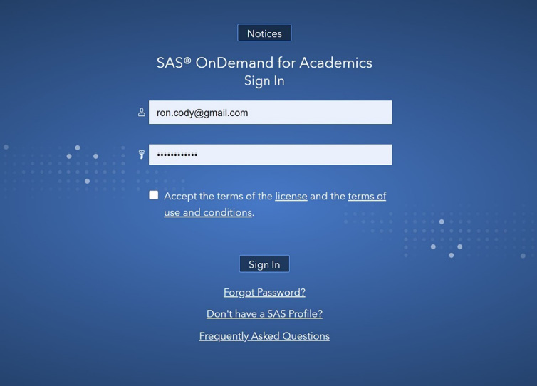
You need to check the box labeled “Accept the terms of the license and the terms of use and conditions.” Once that is completed, click the box labeled Sign In.
The opening screen in SAS Studio looks like this.
Figure 2.2: Opening Screen for SAS Studio
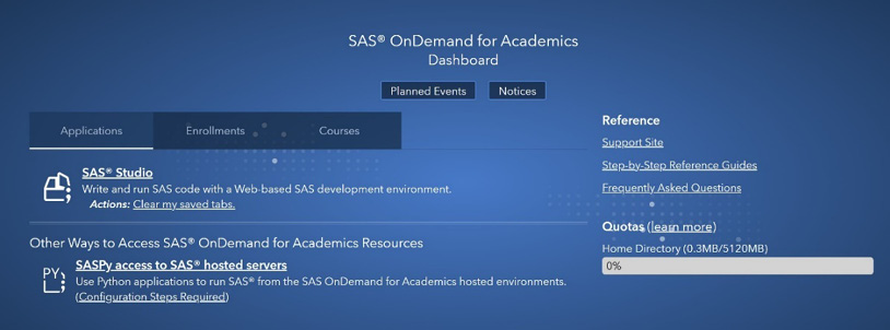
Click SAS Studio to begin your session.
After a few seconds, you arrive at the home screen (yours might vary because this author has already created files and folders).
Figure 2.3: Home Screen for SAS Studio
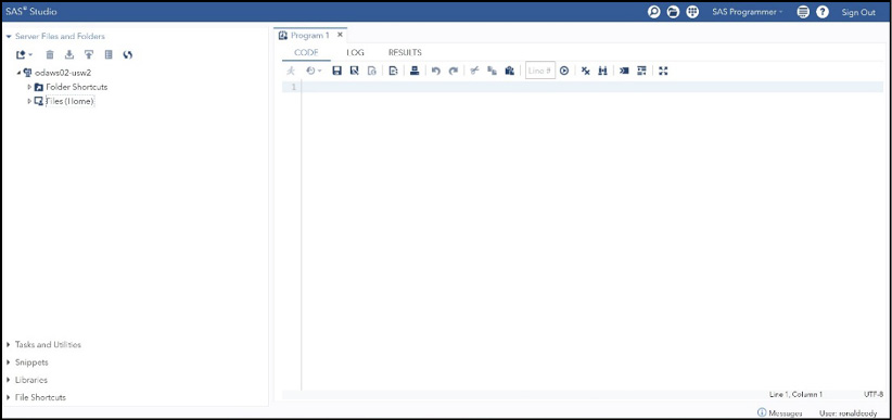
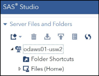
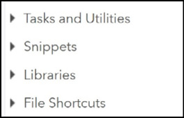
On the left, you see the navigation pane—on the right, the work area. Here is a blow up of the navigation pane:
Figure 2.4: Blow Up of the Navigation Pane
Exploring the Built-In Data Sets
SAS libraries are where SAS stores SAS data sets. SAS Studio ships with a number of data sets that you can play with. In the next chapter, you will see how to create your own SAS data sets from several different data sources and store them in a library of your own.
First click the Libraries tab. Next click the My Libraries tab, you will see something like this.
Figure 2.5: Expanding the My Libraries Tab
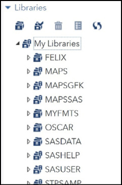
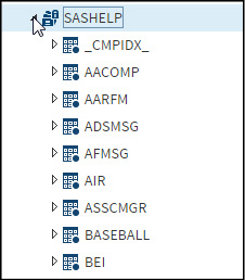
Some of the libraries that you see here were created by the author. Others, such as SASUSER and SASHELP, will always show up. The SASHELP library is where SAS has stored all of the demonstration data sets. Click the small triangle to the left of SASHELP to see a list of the SAS data sets stored there. It should look like Figure 2.6 below.
Figure 2.6: Expanding the SASHELP Library
You can click the small triangle to the left of any of these data sets to see a list of variables. As an alternative, double-click a data set of interest to display a list of variables and a partial listing of the data set. For this example, let’s double-click the BASEBALL data set. Here’s what happens.
Figure 2.7: Opening the BASEBALL Data Set
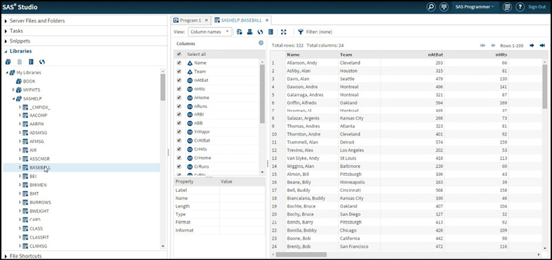
The middle pane shows a list of variables while the right pane shows a partial listing of the data. For a better view of the list of variables, the next figure shows an expanded view.
Figure 2.8: Expanded View of the Variables Pane
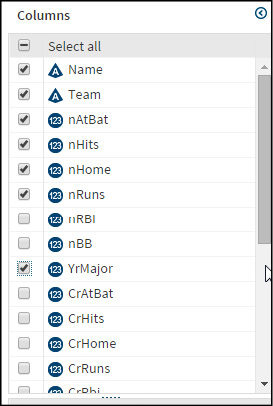
When the data set is displayed, all the variables are selected. You can click any variable to deselect it or, alternatively, uncheck Select All and then, holding down the Ctrl key, select the variables that you want to display. If the variables that you want to select are in sequence, you can also click the first variable of interest, hold the Shift key down, and then click the last variable in the list to select all the variables from the first to the last.
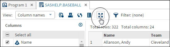
As you select or deselect variables, the work area changes to reflect these selections. Let’s look at the work area with the variable selection shown in Figure 2.8. To enlarge the work area, click the Expand icon (shown below) to expand this area.
Figure 2.9: Expanding the Work Area
The work area is now enlarged and shown in Figure 2.10 below.
You can expand or collapse other panes by clicking on the Expand icon or, if already expanded, on the Collapse icon.
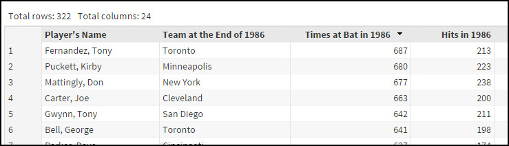
Figure 2.10: Work Area with Selected Variables
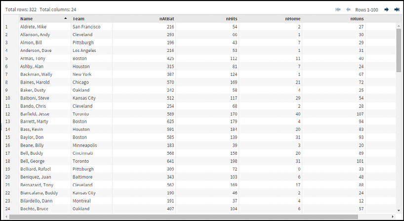
You can use the scroll bars to scroll left or right, up or down. At the top of the work area, you see the number of rows (observations) and columns (variables) in the data set. Here is an enlarged view.
Figure 2.11: Number of Rows and Columns
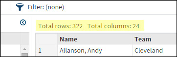
You see that there are 322 rows and 24 columns. These numbers will change as you change your variable selections or create filters.
If you place the cursor on a column heading, an arrow appears. (See Figure 2.12.)Figure 2.12: Placing the Cursor on a Column Heading
Figure 2.12: Placing the Cursor on a Column Heading
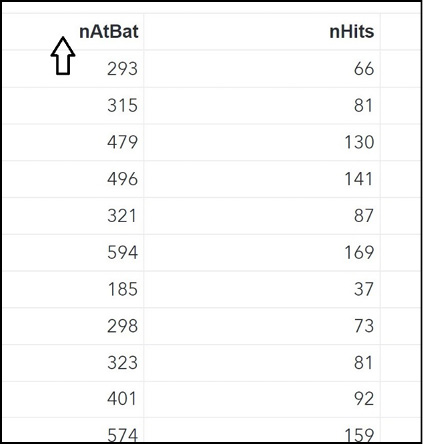
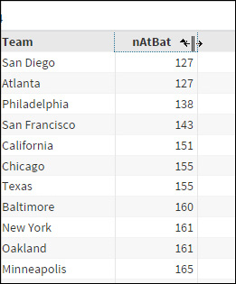
By clicking anywhere in the column heading (the column heading nAtBat stands for the number of times at bat), the values are sorted from low to high (an ascending sort). See Figure 2.13 below.
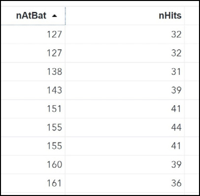
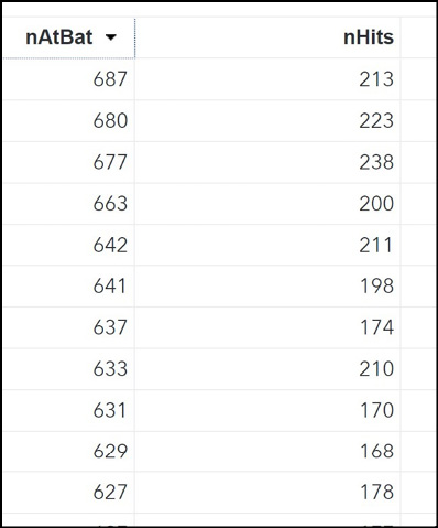
You can click the triangle to the right of the column name to request a descending sort (see Figure 2.14).
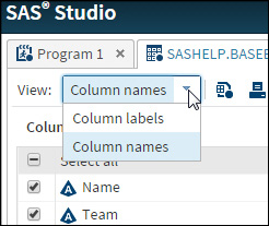
Switching between Column Names and Column Labels
SAS has been the premier data analysis language since computer variables were limited to only 8 characters (now SAS variable names can be 32 characters long). To fix the short variable name problem, long ago, SAS created labels that could be used to identify variables in addition to the variable names. You must use variable names in your programming statements, but you can ask SAS to display the longer, and informative labels (that you must create), when columns of data are presented in reports.
You can switch between variable names and variable labels by clicking on the View tab.
Figure 2.15: Selecting Variable Names or Labels
If you choose column labels, the column names are replaced by labels. (This only works, of course, if the person creating the data set created labels for the variables.) Figure 2.16 shows the effect of switching to column labels for the BASEBALL data set (that did contain labels):
Figure 2.16: Column Headings Changed to Labels
By placing the cursor on the dividing line between columns, the pointer changes to double vertical lines, enabling you to then drag the border of the column left or right. In Figure 2.17 below, the nAtBat column was resized (made smaller).
Figure 2.17: Resizing a Column
Right-clicking a column brings up the following menu.
Figure 2.18: Adding a Filter
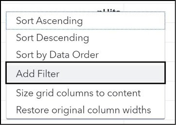
Figure 2.18 shows that you can perform ascending or descending sorts (the same as clicking a column heading). You can do things such as sort in data order, add a filter, or resize columns. Filters are very useful in exploring the data because they enable you to subset rows of the table by specifying criteria, such as displaying only rows where the number of home runs was 30 or more. The following screen shows how to create a filter. Click Add Filter to display the screen shown next.
Figure 2.19: Adding a Filter (Continued)
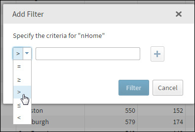
In the drop-down menu, select a logical operator. In this example, you are choosing greater than.
Figure 2.20: Adding a Filter (Continued)
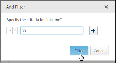
Next, enter a criterion for the variable that you have selected. If you choose a categorical variable like Team, then the filter dialog box gives you the list of values from which you can select. If you want to add more conditions, click the + (plus) sign. If you are finished, click Filter to complete your request.
Figure 2.21: Listing of Filtered Data
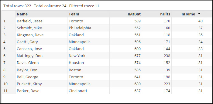
In Figure 2.21, you see all rows in the BASEBALL data set where the player hit more than 30 home runs.
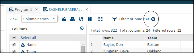
If you want to remove the filter, click the X next to the filter, as shown in Figure 2.22.
Figure 2.22: Removing a Filter
In this chapter, you saw how to open one of the built-in SASHELP data sets and the various tasks that you can perform using simple point-and-click operations supplied by SAS Studio. The next step is to create SAS data sets using your own data and then perform operations such as summarizing your data, creating plots and charts, and creating reports in HTML, PDF, or RTF format. You will learn how to accomplish all of these operations in the chapters to follow.