Chapter 5: Summarizing Data Using SAS Studio
This chapter demonstrates how to summarize numeric and character data. For numeric variables, you will see how to compute statistics such as means and standard deviations, as well as histograms. For character variables, you will see how to generate frequency distributions and bar charts.
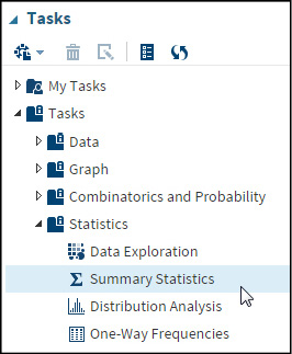
One of the most useful tasks for summarizing numeric data is found on the Statistics task list. Don’t be alarmed that this task is listed under statistics—you don’t need to be a statistician to understand how this works. Expand the Statistics task and select Summary Statistics, as shown in Figure 5.1: Summary Statistics below.
Figure 5.1: Summary Statistics
Double-click Summary Statistics to bring up the DATA and OPTIONS tabs (Figure 5.2).
Figure 5.2: The Summary Statistics Task
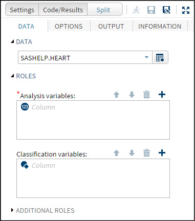
Let’s choose the Heart data set in the SASHELP library to demonstrate how to use the Summary Statistics task. Looking at Figure 5.2: The Summary Statistics Task, you see that SASHELP.Heart has already been chosen. You can click the Data Table icon to select a library and data set that you want to use. The next step is to select the variables that you want to summarize.
Figure 5.3: Selecting Variables

Click the plus sign in the Analysis Variables window and select the variables that you want to analyze (using the Ctrl or Shift keys, as described previously). Notice that the variable list contains only numeric variables. For this example, you have chosen the variables Height, Weight, Diastolic (diastolic blood pressure), and Systolic (systolic blood pressure). Click OK when you are done selecting variables.
You can click the Run icon now or customize the report by clicking on the OPTIONS tab. Let’s do that. It brings up the following screen.
Figure 5.4: Selecting Options
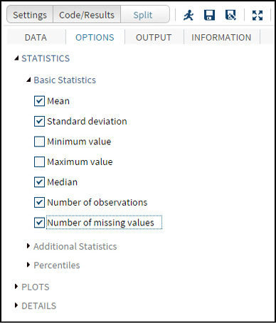
Select or deselect the options that you want. This author recommends that you select the two options—Number of observations and Number of missing values—as they are quite useful. At this point, you can run the task or continue on to request plots. Let’s do that.
Figure 5.5: Plots
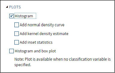
You have the option to include a histogram or a histogram with a box plot. In this example, you have chosen a histogram. If you are statistically minded, you can add a normal density curve and a kernel density estimate. The third option in this list places summary statistics in an inset window in the histogram.
It’s time to run the task. The first part of the output shows the statistics that you requested in tabular form. It looks like this.
Figure 5.6: Tabular Output

Here you see the mean, standard deviation, and median for the selected variables. The last two columns, labeled N and N Miss, show the number of nonmissing observations and the number of missing values for all of your variables, respectively.
To economize on space in this book, only one histogram (Height) is displayed. It looks like this.
Figure 5.7: Histogram
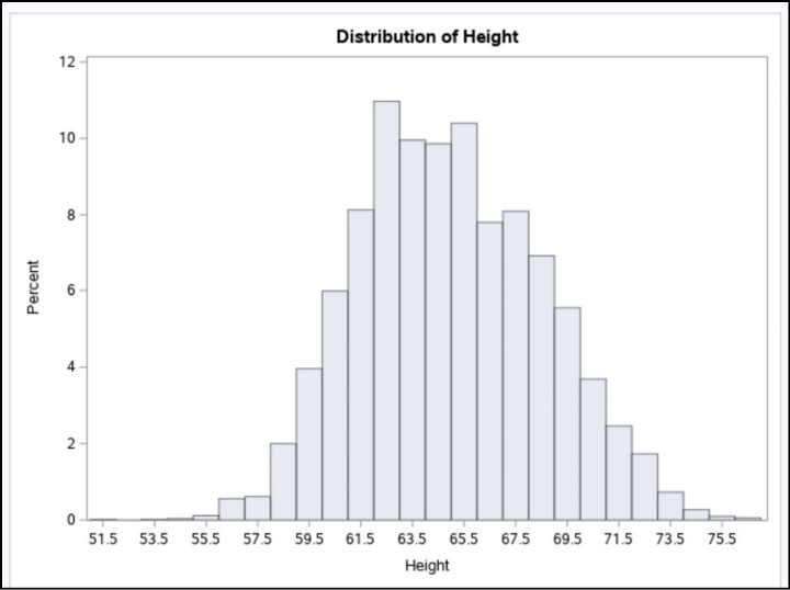
You can use the scroll bars to move right or left, up or down. You can also click the Expand icon to see the entire histogram.
Adding a Classification Variable
The statistics that you have seen so far are computed on the entire data set. To see statistics broken down by one or more classification variables, add those variables in the Classification variables box. To demonstrate this, let’s see the statistics for Height, Weight, Diastolic, and Systolic broken down by the variable Sex. In the DATA tab, click the plus sign in the Classification variables box and select the variable Sex (Figure 5.8).
Figure 5.8: Adding a Classification Variable
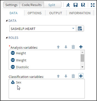
Now run the program to see the following table:
Figure 5.9: Output Showing Classification Data

You see all of the statistics you originally requested for each value of Sex. If you requested plots, you will see separate histograms for each value of the classification variable. To save space, only the histogram for Height is displayed (Figure 5.10).
Figure 5.10: Separate Histograms by Sex
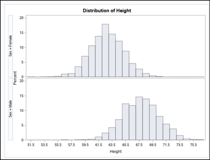
Seeing the two histograms juxtaposed like this is useful in determining if there are differences in the analysis variable for each level of the classification variable.
Summarizing Character Variables
You can use the One-Way Frequencies task to compute counts and percentages for character or numeric variables. If you include any numeric variables in your selection, this task computes frequencies for every unique value of those variables. That is why this task is usually reserved for character variables or for numeric variables with very few unique values.
The first step is to double-click the One-Way Frequencies task.
Figure 5.11: One-Way Frequencies
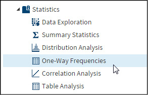
This brings up the screen shown below.
Figure 5.12: One-Way Frequencies Task
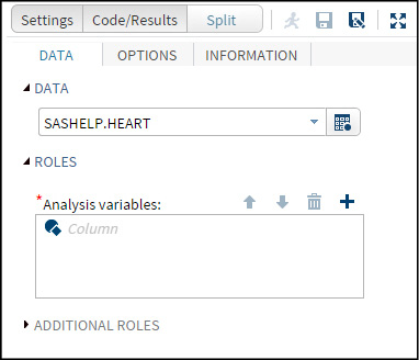
The SASHELP.Heart data set has already been selected. Click the plus sign attached to the Analysis variables box. Then select the variables for which you want to compute frequencies. For this demonstration, the variables Sex, Chol_Status, BP_Status, and Smoking_Status were chosen (the variable Sex is farther up the list and does not appear in Figure 5.13).
Figure 5.13: Selecting Variables
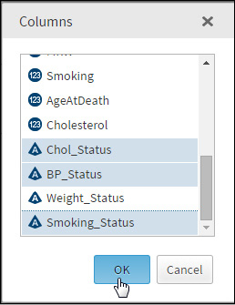
Click OK to proceed. If you want to customize the frequency table, click the OPTIONS tab. This brings up the following:
Figure 5.14: Frequency Options
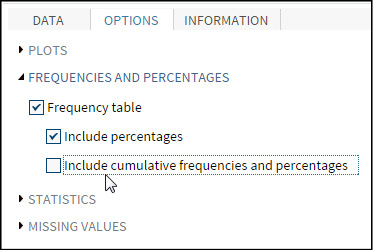
Here, you are deselecting the option to include cumulative frequencies and percentages. (The default is to include cumulative frequencies and percentages.) If you expand the PLOTS option, you will see that the default action is to produce plots. Select the option Suppress plots if you do not want bar charts. In this example, the Suppress plots option is left unchecked.
Figure 5.15: Suppress Plots

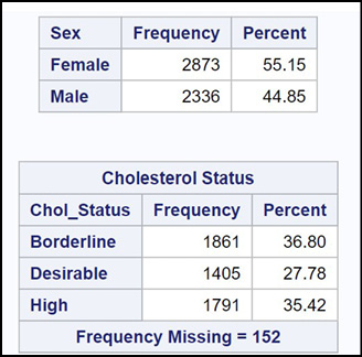
Click the Run icon to complete the task. The output consists of frequency tables and bar charts. Figure 5.16 shows two of the four tables requested. Notice that cumulative frequencies and cumulative percentages are not included (because you unchecked the option to do this).
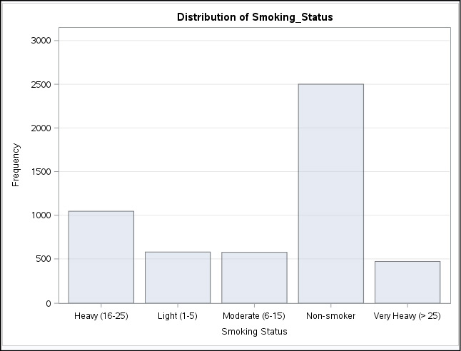
Only one bar chart (for Smoking_Status) is displayed here (Figure 5.17).
The two statistics tasks, Summary Statistics and One-Way Frequencies, can be used to summarize numeric and character data, respectively. You can customize the tabular and graphical output by selecting options for both tasks.