From Toole and Olive (1994).
First, let me express a personal view on word usage. It has to do with the common expression “subjective listening tests.” Of course, they are “subjective” because they involve “listening.” But staying with word usage, it may seem oxymoronic to place the words subjective and measurements in such proximity. However, when it is possible to generate numerical data from listening tests, and those numbers exhibit relatively small variations and are highly repeatable, the description seems to fit. I recall noting this in my very early double-blind listening tests when I employed the simplest metric of variation: standard deviation. In those days, using a 10-point scale of “fidelity,” the very best listeners were repeating their ratings over extended periods of time, with standard deviations around 5%. I found this remarkable, because at that time analog VOM (volt-ohm-milliammeter) multi-testers had similar specifications. Yes, these were measurements. Humans can be remarkable “measuring instruments” if you give them a chance.
This, more than anything else, has allowed the exploration of correlations between technical measurements and subjective opinions. Technical measurements, after all, don’t change, but however accurate and repeatable they may be, they are useless without a method of interpreting them. We need a way to present them to our eyes so they relate more closely to what we hear with our ears: perceptions.
Subjective measurements provide the entry point to understanding the psychoacoustic relationships. The key to getting useful data from listening tests is in controlling or eliminating all factors that can influence opinions other than the sound itself. This is the part that has been missing from most of the audio industry, contributing to the belief that we cannot measure what we hear.
In the early days, it was generally thought that listeners were recognizing excellence and rejecting inferiority when judging sound quality. Regular concertgoers and musicians were assumed to be inherently more skilled as listeners. As logical as this seemed, it was soon thrown into question when listeners in the tests showed that they could rate products just as well with studio-created popular music as they could with classical music painstakingly captured with simple microphone setups, and sometimes even better. How could this be possible? None of us had any idea how the studio creations should sound, with all of the multitrack, close-miked, pan-potted image building and signal processing that went into them. The explanation was in the comments written by the listeners. They commented extravagantly on the problems in the poorer products, heaping scorn rich in adjectives and occasional expletives on things that were not right about the sound. In contrast, high-scoring products received only a few words of simple praise.
And what about musicians? Their performances in listening tests were not distinctive. Some had the occupational handicap of hearing loss; others were clearly more interested in the music than in the sound, and could find “valid interpretations” of instrumental sound in even quite poor loudspeakers. The best among them often had audio as a hobby (Gabrielsson and Sjögren, 1979; Toole, 1985).
People seemed to be able to separate what the loudspeakers were doing to the sound from the sound itself. The fact that, from the beginning, all the tests were of the “multiple-comparison” type may have been responsible. Listeners were able to freely switch the signal among three or four different products while listening to the music. Thus, the “personalities” of the loudspeakers were revealed through the ways the program changed. In a single-stimulus, take-it-home-and-listen-to-it kind of test, this would not be obvious. Isolated A vs. B comparisons fail to reveal problems that are common to both test sounds. The experimental method matters.
Humans are remarkably observant creatures, and we use all our sensory inputs to remain oriented in a world of ever-changing circumstances. So when asked how a loudspeaker sounds, it is reasonable that we instinctively grasp for any relevant information to put ourselves in a position of strength. In an extreme example, an audio-savvy person could look at the loudspeaker, recognize the brand and perhaps even the model, remember hearing it on a previous occasion and the opinion formed at that time, perhaps recall a review in an audio magazine and, of course, would have at least an approximate idea of the cost. Who among us has the self-control to ignore all of that and to form a new opinion simply based on the sound?
It is not a mystery that knowledge of the products being evaluated is a powerful source of psychological bias. In comparison tests of many kinds, especially in wine tasting and drug testing, considerable effort is expended to ensure the anonymity of the devices or substances being evaluated. If the mind thinks that something is real, the appropriate perceptions or bodily reactions can follow. In audio, many otherwise serious people persist in the belief that they can ignore such non-auditory factors as price, size, brand and so on.
This is especially true in the few “great debate” issues, where it is not so much a question of how large a difference there is but whether there is a difference (Clark, 1981, 1991; Lipshitz, 1990; Lipshitz and Vanderkooy, 1981; Nousaine, 1990; Self, 1988). In controlled listening tests and in measurements, electronic devices in general, speaker wire and audio-frequency interconnection cables are found to exhibit small to non-existent differences. Yet, some reviewers are able to write pages of descriptive text about audible qualities in detailed, absolute terms. The evaluations reported on were usually done without controls because it is believed that disguising the product identity prevents listeners from hearing differences. In fact, some audiophile publications heap scorn on double-blind tests that fail to confirm their opinions—the data must be wrong.
Now high-resolution audio has become a “great debate” issue, where it has come down to a statistical analysis of blind test results to reveal whether there is an audible difference and if that difference results in a preference. Meanwhile, some “authorities” claim that it is an “obvious” improvement. As I review the numerous objective tests and controlled subjective results, if there is a difference, it is very, very small, and only a few people can hear it, even in a concentrated comparison test. A difference does not ensure a superior listening experience—that is another level of inquiry. At this point, I lose interest because there are other unsolved problems that are easily demonstrated to be audible, and even annoying. I have dedicated my efforts to solving the “10 dB” problems first, the “5 dB” problems next, and so on. There are still some big problems left. So, unless audiophiles en masse are spending money that should go to feeding their families, these are all simply “great debates” that will energize discussions for years to come.
Science is routinely set up as a “straw man,” with conjured images of wrongheaded, lab-coated nerds who would rather look at graphs than listen to music. In a lifetime of doing audio research, I have yet to find such a person. Rational researchers fully acknowledge that the subjective experience is “what it is all about,” and they use their scientific and technical skills to find ways to deliver rewarding experiences to more people in more places. If something sounds “wrong,” it is wrong. The task is to identify measurements that explain why it sounds wrong and, more importantly, to identify those measurements that contribute to it sounding “right.”
In the category of loudspeakers and rooms, however, there is no doubt that differences exist and are clearly audible. Because of this, most reviewers and loudspeaker designers feel that it is not necessary to go to the additional trouble of setting up blind evaluations of loudspeakers. This attitude has been tested.
When I joined Harman International, listening tests were casual affairs, as they were and still are in many audio companies. In fact, a widespread practice in the industry has been that a senior executive would have to sign off on a new product, whether they were good listeners or not. After engineers had sweated the design details to get a good product, they might be told, “more bass, more treble, and can you make it louder?” Simply sounding “different” on a showroom floor was considered to be an advantage, and sounding louder was a real advantage given that few stores did equal-loudness comparisons. Some managers even had imagined insights into what the purchasing public would be listening for in the upcoming shopping season. In certain markets a prominent product reviewer might be invited to participate (usually for pay) in a “voicing” session to ensure a good launch of a new product. The final product may or may not have incorporated the advice, and it is unlikely that the deception would ever be discovered.
It was a grossly unscientific process, unjust to the efforts of competent engineers and disrespectful of the existing science, and it contributed to unnecessary variations in product “sounds.” Many consumers think that there is a specific “sound” associated with a specific brand. That can happen, but it is not universal and not really very consistent, even if that is what was intended. If you reflect on the circle of confusion (Section 1.4), this does nothing to improve the chances of good sound being delivered to customers. There has to be a better way.
With the demise of so many enthusiast audio stores, consumers have few opportunities to listen for themselves, and almost never in circumstances that might lead to a fair appraisal of products. Shopping is migrating to the Internet, and consumers increasingly rely on Internet audio forum opinions and product reviews. Clearly, there is a need for minimally biased subjective evaluations, and for useful measurements that consumers might eventually begin to trust.
Music composition and arrangement involves voicing to combine various instruments, notes and chords to achieve specific timbres. Musical instruments are voiced to produce timbres that distinguish the makers. Pianos and organs are voiced in the process of tuning, to achieve a tonal quality that appeals to the tuner or that is more appropriate to the musical repertoire. This is all very well, but what has it to do with loudspeakers that are expected to accurately reproduce those tones and timbres?
It shouldn’t be necessary if the circle of confusion did not exist, and all monitor and reproducing loudspeakers were “neutral” in their timbres. However, that is not the case, and so the final stage in loudspeaker development often involves a “voicing” session in which the tonal balance is manipulated to achieve what is hoped to be a satisfactory compromise for a selection of recordings expected to be played by the target audience. There are the “everybody loves (too much) bass” voices, the time-tested boom and tizz “happy-face” voices, the “slightly depressed upper-midrange voices” (compensating for overly bright close-miked recordings, and strident string tone in some classical recordings), the daringly honest “tell it as it is” neutral voices and so on. It is a guessing game, and some people are better at it than others. It is these spectral/timbral tendencies that, consciously or unconsciously, become the signature sounds of certain brands. Until the circle of confusion is eliminated, the guessing game will continue, to the everlasting gratitude of product reviewers, and to the frustration of critical listeners. It is important for consumers to realize that it is not a crime to use tone controls. Instead, it is an intelligent and practical way to compensate for inevitable variations in recordings, that is, to “revoice” the reproduction if and when necessary. At the present time, no loudspeaker can sound perfectly balanced for all recordings.
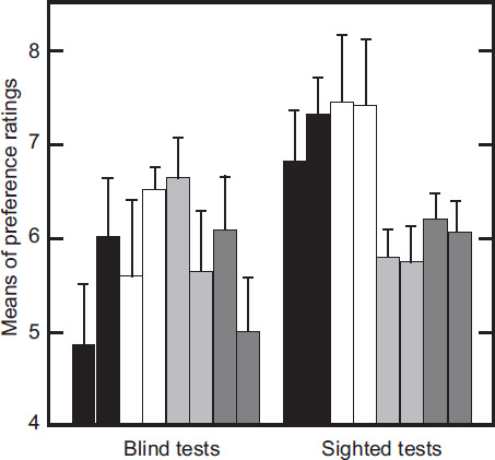
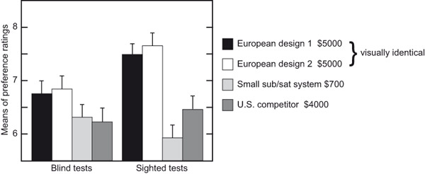
Continuing the Harman story, a blind test facility was set up and the engineers were encouraged to incorporate competitive evaluations into the product development routine. Some went along with the plan of striving to be “best in class,” using victory in the listening test as the indicator that the design was complete. However, a few engineers regarded the process as an unnecessary interruption of their work, and a challenge to their own judgment. At a certain point it seemed appropriate to conduct a test—a demonstration that there was a problem. It would be based on two listening evaluations that were identical, except one was blind and one was sighted (Toole and Olive, 1994).
Forty listeners participated in a test of their abilities to maintain objectivity in the face of visible information about products. All were Harman employees, so brand loyalty would be a bias in the sighted tests. They were about equally divided between experienced listeners, those who had previously participated in controlled listening tests, and inexperienced listeners, those who had not.
Figure 3.1 shows that in the blind tests, there were two pairs of statistically indistinguishable loudspeakers: the two European “voicings” of the same hardware and the other two products. In the sighted version of the test, loyal employees gave the big, attractive Harman products even higher scores. However, the little, inexpensive sub/sat system dropped in the ratings; apparently its unprepossessing appearance overcame employee loyalty. Obviously, something small and made of plastic cannot compete with something large and stylishly crafted of highly polished wood. The large, attractive competitor improved its rating but not enough to win out over the local product. It all seemed very predictable. From the Harman perspective, the good news was that two products were absolutely not necessary for the European marketing regions. (So much for intense arguments that such a sound could not possibly be sold in [pick a country].) In general, seeing the loudspeakers changed what listeners thought they heard.
The effects of room position on sound quantity and quality at low frequencies are well documented. It would be remarkable if these did not reveal themselves in subjective evaluations. This was tested in a second experiment where the loudspeakers were auditioned in two locations that would yield quite different sound signatures. Figure 3.2 shows that listeners responded to the differences in blind evaluations: adjacent bars of the same color have different heights, showing the different ratings when the loudspeaker was in position 1 or 2. In contrast, in the sighted tests, things are very different. First, the ratings assume the same pattern that was evident in the first experiment; listeners obviously recognized the loudspeakers and recalled the ratings they had been given in the first experiment (Figure 3.1). Second, they did not respond to the previously audible differences attributable to position in the room; adjacent bars have closely similar heights. Third, some of the error bars are quite short; no thought is required when you know what you are listening to. Interestingly, the error bars for the two visually identical “European” models (on the left) were longer because the eyes did not convey all of the necessary information.
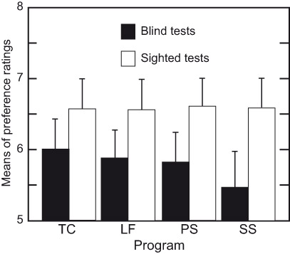
It is normal to expect an interaction between the preference ratings and individual programs. In Figure 3.3 this is seen in the results of the blind tests, where the data have been arranged to show declining scores for programs toward the right of the figure. In the sighted versions of the tests, there are no such changes. Again, it seems that the listeners had their minds made up by what they saw and were not in a mood to change, even if the sound required it. In a special way, they went “deaf.” The effect is not subtle.
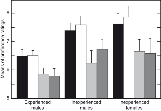
Dissecting the data and looking at results for listeners of different genders and levels of experience, Figure 3.4 shows that experienced males (there were no females who had participated in previous tests) distinguished themselves by delivering lower scores for all of the loudspeakers. This is a common trend among experienced listeners. Otherwise, the pattern of the ratings was very similar to those provided by inexperienced males and females. Over the years, female listeners have consistently done well in listening tests, one reason being that they tend to have closer to normal hearing than males (noisy work environments, or hobbies?). Lack of experience in both sexes shows up mainly in elevated levels of variability in responses (note the longer error bars), but the responses themselves, when averaged, reveal patterns similar to those of more experienced listeners. With experienced listeners, statistically reliable data can be obtained in less time.
Summarizing, it is clear that knowing the identities of the loudspeakers under test can change subjective ratings.
These findings mean that if one wishes to obtain candid opinions about how a loudspeaker sounds, the tests must be done blind. The answer to the question posed in the title of this section is “yes.” The good news is that if the appropriate controls are in place, experienced and inexperienced listeners of both genders are able to deliver useful opinions. Inexperienced listeners simply take longer and more repetitions to produce the same confidence levels in their ratings.
Opinions of sound quality are based on what we hear, so, if hearing is degraded we simply don’t hear everything, and opinions will change. Hearing loss is depressingly common, and the symptoms vary greatly from person to person, so opinions from such persons are simply their own, and they may or may not be relevant to others.
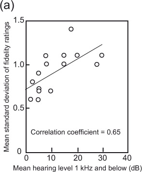
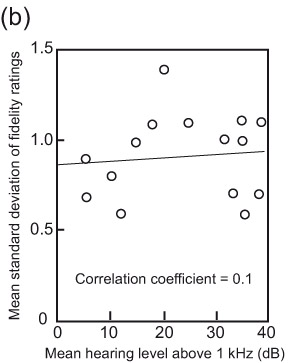
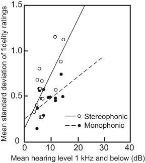
The first clear evidence of the issue with hearing came in 1982 during an extensive set of loudspeaker evaluations conducted for the Canadian Broadcasting Corporation (CBC), in which many of the participants were audio professionals: recording engineers, producers, musicians. Sadly for them, hearing loss is an occupational hazard (discussed in Chapter 17). During analysis of the data, it was clear that some listeners delivered remarkably consistent overall sound quality ratings (then called fidelity ratings, reported on a scale ranging from 0 to 10) over numerous repeated presentations of the same loudspeaker. Others were less good, and still others were extremely variable—liking a product in the morning and disliking it in the afternoon, for example. The explanation was not hard to find. Separating listeners according to their audiometric performances, it was apparent that those listeners with hearing levels closest to the norm (0 dB) had the smallest variations in their judgments. Figure 3.5 shows examples of the results. Surprisingly, it was not the high-frequency hearing level that correlated with the judgment variability but that at frequencies at or below 1 kHz. Bech (1989) confirmed the trend.
Noise-induced hearing loss is characterized by elevated thresholds around 4 kHz. Presbycusis, the hearing deterioration that occurs with age, starts at the highest frequencies and progresses downward. These data showed that by itself, high-frequency hearing loss did not correlate well with trends in judgment variability (see Figure 3.5b). Instead, it was hearing level at lower frequencies that showed the correlation (Figure 3.5a). Some listeners with high-frequency loss had normal hearing at lower frequencies, but all listeners with low-frequency hearing loss also had loss at high frequencies—in other words, it was a broadband problem. We now know that elevated hearing thresholds are often accompanied by reduced ability to separate sounds in space, which would include separating the listening room from the sound of the loudspeaker, which adds significant difficulty to the task. This is very likely a broadband effect.
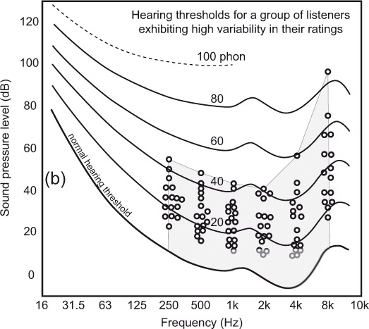
Illustrating the situation more clearly is Figure 3.6, which displays the hearing performance of the author as a function of age, and a collection of threshold measurements for the high-variability listeners in Figure 3.5. The hearing threshold data are shown superimposed on the family of equal-loudness contours, the sound levels at which different pure tones are judged to be equally loud. The bottom curve is the hearing threshold, below which nothing is heard. A detailed explanation is in Section 4.4.
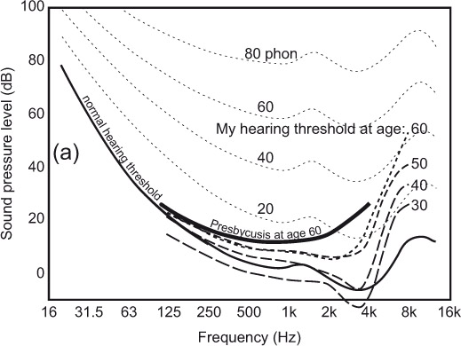
Adapted from Toole (1985), figure 7. Equal loudness contours are from ISO 226 (2003). © ISO. This material is adapted from ISO 226.2003 with permission of the American National Standards Institute (ANSI) on behalf of the International Organization for Standardization (ISO). All rights reserved.
My thresholds at age 30 were slightly below (better than) the statistical average. With age, and acoustical abuses of various kinds, the hearing level rose gradually, most dramatically at high frequencies. Even so, my deterioration was less than the population average presbycusis for age 60. My broadband auditory dynamic range was degraded by only 10 dB or so over those years, except that high frequencies disappeared at a higher rate.
In contrast, the professional audio people whose audiometric data are shown in Figure 3.6b were unable to hear large portions of the lower part of the dynamic range. Without the ability to hear small acoustical details in music and voices (good things) or low-level noises and distortions (bad things), these people were handicapped in their abilities to make good or consistent judgments of sound quality, and this was revealed in their inconsistent ratings of products. It did not prevent them from having opinions, deriving pleasure from music, or being able to write articulate dissertations on what they heard, but their opinions were not the same as those of normal hearing persons. Consequently, future listeners underwent audiometric screening, and those with broadband hearing levels in excess of about 20 dB were discouraged from participating.
All of this emphasis on normal hearing seems to imply that a criterion excluding listeners with a greater than 15–20 dB hearing level may be elitist. According to USPHS (US Public Health Service) data, about 75% of the adult population should qualify. However, there is some concern that the upcoming generations may not fare so well because of widespread exposure to high sound levels through headphones and other noisy recreational activities.
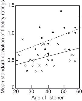
Hearing loss occurs as a result of age and accumulated abuse over the years. Whatever the underlying causes, Figure 3.7 shows that in terms of our ability to make reliable judgments of sound quality, we do not age gracefully. A couple of the data points indicate that young persons are not immune to hearing loss. It certainly is not that we don’t have opinions or the ability to articulate them in great detail; it is that the opinions themselves are less consistent and possibly not of much use to anyone but ourselves. In my younger years, I was an excellent listener—one of the best, in fact. However, listening tests as they are done now track not only the performance of loudspeakers but of listeners—the metric shown in Figure 3.9. At about age 60, it was clear that it was time for me to retire from the active listening panel. Variability had climbed and, frankly, I found it to be a noticeably more difficult task. It is a younger person’s pursuit. Music is still a great pleasure, but my opinions are now my own. When graybeards expound on the relative merits of audio products, they may or may not be relevant. But be polite—the egos are still intact.
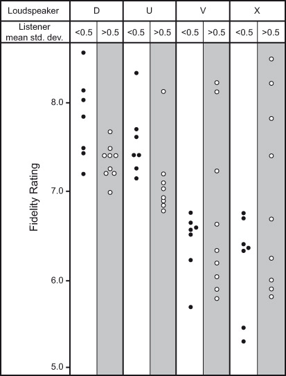
Figure 3.8 shows results for individual listeners who evaluated four loudspeakers in a monophonic multiple-comparison blind test. Why mono? The explanation is in the next section. Multiple-comparison test? All four loudspeakers were available to be heard by the listener, switched at will at the push of a button. Loudness levels were normalized. Each dot is the mean of several judgments on each of the products, made by one listener. To illustrate the effect of hearing level on ratings, listeners were grouped according to the variability in their judgments: those who exhibited standard deviations below 0.5 scale unit and those above that. The low-variability listener results are shown in the white areas and the high-variability results are in the shaded areas. Obviously, the inference is that the ratings shown in the shaded areas are from listeners with less than normal hearing.
In Figure 3.8, it is seen that fidelity ratings for loudspeakers D and U are closely grouped by both sets of listeners, but the ratings in the shaded areas are simply lower. Things change for loudspeakers V and X, where the close groupings of the low-variability listeners contrast with the widely dispersed ratings by the high-variability listeners. This is a case where an averaged rating does not reveal what is happening. Listener ratings simply dispersed to cover the available range of values; some listeners thought it was not very good (fidelity ratings below 6), whereas others thought it was among the best loudspeakers they had ever heard (fidelity ratings above 8). Listeners simply exhibited strongly individualistic opinions. Hearing loss is very likely involved. Be careful whose opinions you trust.
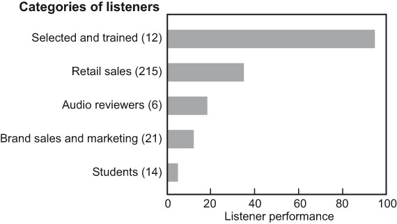
Other investigations agree. Bech (1992) observed that hearing levels of listeners should not exceed 15 dB at any audiometric frequency and that training is essential. He noted that most subjects reached a plateau of performance after only four training sessions. At that point, the test statistic FL should be used to identify the best listeners. Olive (2003) compiled data on 268 listeners and found no important differences between the ratings of carefully selected (for normal hearing) and trained (to be able to recognize resonances) listeners and those from several other backgrounds—some in audio, some not, some with listening experience, some with none. There were, as shown in Figure 3.9, huge differences in the variability and scaling of the ratings, so selection and training have substantial benefits in time savings. Rumsey et al. (2005) also found strong similarities in ratings of audio quality, anticipating only a 10% error in predicting ratings of naïve listeners from those of experienced listeners.
The good news for the audio industry is that if a loudspeaker is well designed, ordinary customers may recognize it—if given a reasonable opportunity to judge. The pity is that there are few opportunities to make valid listening comparisons in retail establishments, and the author is not aware of an independent source of such unbiased listening test data for customers to go to for help in making purchasing decisions.
It is paradoxical that opinions of reviewers are held in special esteem. Why are these people in positions of such trust? The listening tests they perform violate the most basic rules of good practice for eliminating bias. They offer us no credentials, no proofs of performance, not even an audiogram to tell us that their hearing is not impaired. Adding to the problem, most reviews offer no meaningful technical measurements so that readers might form their own impressions.
Fortunately, it turns out that in the right circumstances, most of us, including reviewers, possess “the gift”: the ability to form useful opinions about sound and to express them in ways that have real meaning. All that is needed to liberate the skill is the opportunity to listen in an unbiased frame of mind.
Subjectivists have criticized double-blind testing because it puts extraordinary stress on listeners, thereby preventing their full concentration on the task. This is presumed to explain why these people don’t hear differences that show up in casual listening. Years of doing these tests with numerous listeners have shown that, after a brief introductory period, they simply settle into the task. Regular listeners have no anxiety. Years ago, while at the National Research Council of Canada (NRCC), we routinely contracted to perform anechoic measurements and to conduct blind loudspeaker comparisons for Canadian audio magazines. The journalists traveled to Ottawa, arriving the night before the tests to give their ears a chance to rest, and spent a day or more doing double-blind subjective evaluations before they got to see the measurements on the products they submitted. On one occasion, due to unforeseen circumstances, the acoustically transparent, visually opaque screen was not available—it was on a truck a few hours away. Rather than waste time, it was decided to start the tests without the screen—sighted. A few rounds into the randomized, repetitive tests our customers called a halt to the proceedings—they felt that seeing the loudspeakers prevented them from being objective—they were stressed! They waited for the truck to arrive.
Those of us who have done many of these tests agree. In the end, it is simpler if there is only one task: to judge the sound. There is no need to wonder if one is being influenced by what is seen, noting that certain familiar brand names might not be performing as anticipated, thinking you might be wrong, and so on. And all of us long ago gave up trying to guess what we are listening to—it is another distraction that usually proves to be wrong. In multiple comparison tests it is advisable to add one or more products that are not known to the listeners.
Additional criticisms had to do with notions that the sound samples might be too short for critical analysis, and that a time limit can be stressful. For the past 25+ years the process at Harman has involved single listeners, who select which of the three or four unidentified loudspeakers is to be heard at any time, and there is no time limit—switch at will, and take as long as is needed. The musical excerpts are short, but repeated in nicely segued loops to allow for detailed examination. Stressful?
We listen to almost all music in stereo; that is the norm. So, it makes sense to do double-blind listening tests in stereo too, right? Wrong. It all came to a head back in 1985, when I decided to examine the effects of loudspeaker directivity and adjacent side-wall reflections (Toole, 1985, described in Section 7.4.2). In the process I did tests using one and both of the loudspeakers. Because stereo imaging and soundstage issues were involved, listeners were interrogated on many aspects of spatial and directional interest. To our great surprise, listeners had strong opinions about imaging when listening in mono. Not only that, but they were very much more strongly opinionated about the relative sound quality merits of the loudspeakers in the mono tests than in the stereo tests.
Over the years mono vs. stereo tests have been done to satisfy various doubters. Each time the loudspeaker that won the mono tests also won the stereo tests, but not as convincingly, because in stereo everything tended to sound better. And what about imaging? It turns out to be dependent on the recording and the loudspeaker; there is a strong interaction. Classical recordings, with their high content of “ambiance” (i.e., uncorrelated L and R channel information), tended to be quite unaffected by the loudspeaker. However, some popular and jazz recordings, with close-miked, panned and equalized mixes, exhibited some loudspeaker interactions—as might be expected because they were control-room creations, not capturing a live event. But there were interactions involving specific recordings with specific loudspeakers.
More recently, tests were done that included mono, stereo and multichannel presentations (Olive et al., 2008). The results, shown in Figure 3.10, indicate that when there was a perceived preference among the optional sound qualities, it was most clearly revealed in monophonic listening. As active channels were added to the presentations, the ability to distinguish between sounds of different timbres appeared to deteriorate. Condition “B” was by far the worst sounding option on monophonic listening, with significant resonant colorations, yet, in stereo and multichannel presentations, it was judged to be close to the truly superior systems.
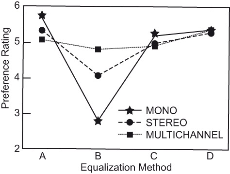
From Olive et al. (2008).
A persuasive justification for monophonic evaluations is the reality that in movies and television programs, the center channel does most of the work—a monophonic sound source. The center channel is arguably the most important loudspeaker in a multichannel system. In popular music and jazz stereo recordings, images are often hard-panned to the left or right loudspeakers, again monophonic sources, and the phantom center image is the product of double mono, identical sounds emerging from L and R loudspeakers.
Finally, the data of Figure 3.11 adds more strength to the argument that monophonic listening has merits. It shows that only those listeners with hearing levels very close to the statistical normal level (0 dB) are able to perform similarly well in both stereo and mono tests. Even a modest elevation in hearing level causes judgment variations in stereo tests to rise dramatically, yielding less-trustworthy data. Age and hearing loss affect one’s ability to separate multiple sounds in space. We may notice this in a crowd or in a restaurant setting, but we may not be aware of the disability when listening to a stereo soundstage (see Section 17.2). The directional and spatial complexity of stereo appears to interfere with our ability to isolate the sound of the loudspeakers.
For program material, some people insist on using one of a stereo pair of channels, but summing the channels is possible with many stereo programs; listen, and find those that are mono compatible. Because complexity of the program is a positive attribute of test music, abandoning a channel is counterproductive.
In summary, while it is undeniable that good stereo and multichannel recordings are more entertaining than monophonic versions, it is an inconvenient truth that monophonic listening provides circumstances in which the strongest perceptual differentiation of sound quality occurs. If the purpose of a listening test is to evaluate the intrinsic sound quality from loudspeakers, listen in mono. For pleasure, or to impress someone, listen in stereo or multichannel modes.
When multiple loudspeakers are simultaneously active, the uncorrelated spatial sounds in the recordings modify the ability of listeners to judge timbral quality. As noted in Section 7.4.2, the sound quality and spatial quality ratings were very similar. Is it possible that these perceived attributes couldn’t be completely separated? As discussed in Section 7.4.4, Klippel found that 50% of listeners’ ratings of “naturalness” were attributed to “feeling of space”; with “pleasantness,” it was 70%. So spatial effects are important—more important than the author anticipated—and forming opinions about sound quality in stereo and multichannel listening is obviously a complex affair.
But aren’t there qualities of a loudspeaker that only show up in stereo listening, because of the many subtle dimensions of “imaging”? One can conceive of loudspeakers with grossly inferior spectral response and/or irregular off-axis performance generating asymmetries in left and right channel sounds. So, possibly there are, but with competently designed loudspeakers the spatial effects we hear appear to be dominated by the information in the recordings themselves. The important localization and soundstage information is the responsibility of the recording engineer, not the loudspeaker, and loudspeakers with problems large enough to interfere with those intentions should be easily recognizable in technical measurements or from their gross timbral distortions. For stereo, the first requirement is identical left and right loudspeakers and left-right symmetry in the room. That requirement is not always met, in which case many forms of audible imperfections may be heard, and the reasons may not be obvious.
The circle of confusion applies also to stereo imaging.
Any measurement requires controls on nuisance variables that can influence the outcome. Some can be completely eliminated, but others can only be controlled in the sense that they are limited to a few options (such as loudspeaker and listener positions) and therefore can be randomized in repeated tests, or they can be held as constant factors. Much has been written on the topic (Toole, 1982, 1990; Toole and Olive, 2001; Bech and Zacharov, 2006). The following is a summary.
As audio enthusiasts know, and as explained in detail in Chapters 8 and 9, rooms have a massive influence on what we hear at low frequencies. There are also effects at higher frequencies, in the reflection of off-axis sounds described by loudspeaker directivity. Therefore, if comparing loudspeakers, listen to all of them in the same room, taking time to let the listeners adapt to the acoustical setting. Listeners have the ability to adapt to many aspects of room acoustics, as long as they are not extreme problems. As explained in Section 8.1.1, there are no “ideal” dimensions for rooms, in spite of claims to the contrary. There are practical dimensions, however, that allow for the proper placement of a stereo pair of loudspeakers and a listener, or of a multichannel array of loudspeakers and a group of listeners.
The importance of blind listening was established in Section 3.1, but how, in practice, is it achieved? An acoustically transparent screen is a remarkable device for revealing truths, but it is essential to test the acoustical transmission loss of the material by performing a simple on-axis frequency response measurement, then place the material between the loudspeaker and microphone, and measure again. There will be a difference, but it should be less than 1 dB, even at the highest frequencies, as it is in a good grille cloth. Polyester double-knit is a commonly available possibility. However, care must be taken to ensure that the fabric when tested and used is under slight tension to open the weave—it is this that is responsible for the acoustical transparency. Because fabrics with low acoustical loss tend to be very porous (easy to blow air through, and to see glints of daylight through) they can reveal outlines and sometimes more of the loudspeakers being evaluated. Minimize the light behind the screen, and emphasize the lighting levels on the audience side to alleviate this problem—directional lighting helps.
Should you listen with the grilles on or off? It depends on your audience. In reality, only audiophile enthusiasts are likely to want to, or can get away with, leaving the transducers exposed. In good products the differences should be vanishingly small, but this is not always so. Conscientious loudspeaker designers include the grille cloth and frame (often the bigger problem) into the design. In the real world, visual aesthetics count for something, and grille cloths are a deterrent to probing fingers.
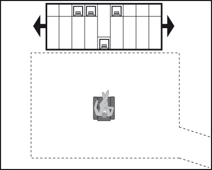
Ideally, use positional substitution: bring the active loudspeakers to the same position so that the coupling to the room modes is constant. This can be expensive, and requires a dedicated facility, something beyond the means of hobbyists, or even audio publications and their reviewers. But, with the expenditure of some time and effort, simpler methods can yield very reliable results. Figure 3.12 shows the listening room used in my original research at the NRCC in the 1980s. In this, three or four loudspeakers were located at the numbered locations, and some number of listeners occupied the seats. Rigorous tests used only a single listener at a time. After each sequence of music, during which listeners made notes and decided on “fidelity” ratings, the loudspeakers were randomly repositioned and the listeners took different seats. This process was repeated until all loudspeakers had been heard in all locations. It was time-consuming, but it reduced the biasing influence of room position, which in some cases could be the deciding factor.
The results were good enough to provide a solid foundation for the research that followed. The setup needs to be calibrated by measurements from each loudspeaker location to each listener location, and positional adjustments made so as to avoid accidental contamination by one or more obtrusive room resonances. The appendix of Toole (1982) describes the process for one room, and Olive et al. (1998), Olive (2009) and McMullin et al. (2015) document others. The room cannot be eliminated, but it should be a relatively constant, and innocuous, factor. If the result is to be an evaluation relevant to ordinary audiophiles or consumers, deliberate acoustical treatment must be moderated. Imitating an “average” domestic listening room is a good objective, and the most contentious decision is likely to be what to do with the first side wall reflection. My initial decision, many years ago, was to let it reflect—a flat, untreated surface, as happens in many domestic rooms and retail demonstrations—so that the off-axis behavior of the loudspeaker would be revealed. This is a demanding test, as it probably should be for loudspeaker evaluations intended to apply to a general population. But, for one’s personal recreational listening there are other factors to consider, as is discussed in Chapter 7.
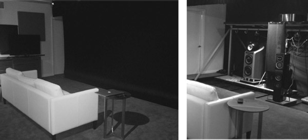
Figures 3.13 and 3.14 show an evolution of those listening tests, the Harman International Multichannel Listening Laboratory (MLL) (Olive et al., 1998). In this, a positional substitution process has been automated using computer-controlled pneumatic rams to move the entire platform left and right, and to move the desired loudspeaker(s) to a predetermined forward location, storing the silent loudspeakers at the rear. The amount of forward movement is programmable, and stereo and L, C, R arrangements can be compared. The positional exchanges take about 3 s, and take place quietly. The single listener controls the process, choosing the active loudspeaker (which has a coded identity) and deciding when it is time to move on to the next musical selection. When the music changes (a random process), the coded identities are randomly changed, so in effect it becomes a new experiment. There is no time limit. All of these functions are computer randomized to make it a true double-blind test.
There are other ingenious ways to achieve positional substitution for in-wall or on-wall loudspeakers, sound bars and so forth. If these tests are to be a way of life, any are worth considering because of the excellent results they yield and the time savings involved. If none of this is possible, a variation of Figure 3.12 certainly works, costs nothing, but involves more work and more time. A simple turntable is another cost-effective and practical solution. It can be operated by a patient volunteer behind the screen (Figure 7.11) or automated (McMullin et al., 2015, figure 14). Versions of these automated movers can be built into walls for evaluating flat-panel TV audio systems, sound bars, on- and in-wall/ceiling loudspeakers, and so forth (Olive, 2009; McMullin et al., 2015).
Many situations do not lend themselves to real-time in situ listening tests. Binaural recordings reproduced at a later time provide an obvious alternative, but many people have a problem accepting the idea that headphone reproduction is a satisfactory substitute for natural listening. The author also had doubts in the beginning, but the appearance of the Etymötic Research ER-1 insert earphones provided what seemed to be a solution to the largest problem: delivering a highly predictable signal to the listeners’ eardrums. Toole (1991) describes the problems in detail, and shows results of early tests in which there was good agreement between real-time and binaural listening tests of some loudspeakers. The same basic process was used in experiments comparing results of listening tests done in different rooms (Section 7.6.2 and Olive et al., 1995). Again the results of real-time and binaurally time-shifted tests yielded closely similar results.
These tests employed a static KEMAR head and torso simulator (an anthropometric mannequin) as a binaural microphone, and a problem was that much or all of the time the sound was perceived to be in-head localized. Playing the binaural recordings in the same room that they were recorded in significantly alleviated this, allowing listeners to see and hear the room before the recorded version took over. In such instances the sounds were often credibly externalized. However, the illusion deteriorated when the listening was done in a different room and what the eyes saw did not match what the ears heard.
A more elaborate scheme called Binaural Room Scanning (BRS) involves measuring binaural room impulse responses (BRIR) at each of many angular orientations of the mannequin in the test environment. For playback, the music signal is convolved with the BRIR filters as it is reproduced through headphones attached to a low-latency head-tracking system. By this means, as the listener’s head rotates, the sounds at the ears are modified so as to maintain a stable spatial relationship with the real room. The result is a much more persuasive externalization of the sound and the associated spatial cues. Olive et al., 2007; Olive and Welti 2009; Welti and Olive, 2013; Gedemer and Welti, 2013; and Gedemer, 2015b, 2016 describe such experiments in domestic rooms, cars and cinemas.
A literature search will reveal many more examples, because binaural techniques are now accepted in audio and acoustical research. A fact not recognized by many skeptics is that this requires a precise knowledge of the sounds that reach the listeners’ eardrums. A carefully calibrated system is required, and headphones or insert earphones are chosen for the ability to deliver predictable sounds to the eardrums.
Listen in the same room, using a single listener in the same location. If there are multiple listeners, on successive evaluations it is necessary to rotate listeners through all of the listening positions. The problem with multiple listeners is avoiding a “group” response. Some people have difficulty muting verbal sounds signaling their feelings, and others may exhibit body language conveying the same message. This is especially true when anyone in the group is respected for his or her opinion. Such listeners sometimes deliberately reveal their opinions verbally or non-verbally, in which case the test is invalid. Single listeners are much preferred and enforce a “no discussion” rule between tests.
Seats should have backs that rise no higher than the shoulders to avoid reflections and shadowing from multichannel surround loudspeakers.
In any listening comparison, louder sounds are perceptually recognizable, which is an advantage for persons looking for a reason to express an opinion. It is a well-known sales strategy in stores. Perceived loudness depends on both sound level and frequency, as seen in the well-known equal-loudness contours (Figure 4.5). Consequently, something as basic as perceived spectral balance is different at different playback levels, especially the important low-bass frequencies. If the frequency responses of the devices being compared are identical, as in most electronic devices, loudness balancing is a task easily accomplished with a simple signal like a pure tone and a voltmeter. Loudspeakers are generally not flat, and individually they are not flat in many different ways. They also radiate a three-dimensional sound field into a reflective space, meaning that it is probably impossible to achieve perfect loudness equality for all possible elements (e.g., transient and sustained) of a musical program.
There has been a long quest for a perfect “loudness” meter. Some of the offerings have been exceptionally complicated, expensive and cumbersome to use, requiring narrow-band spectral analysis and computer-based loudness-summing software. The topic is discussed in Section 14.2.
The practical problem is that if the frequency responses of the loudspeakers (or headphones) being compared are very different, a loudness balance achieved with one kind of signal would not apply to a signal with a different spectrum. Fortunately, as loudspeakers have improved and are now more similar, the problem has lessened, although it has not disappeared. In all of these cases, if in doubt, turn the instruments off and listen; a subjective test is the final authority.
Spectral balance is affected by playback sound levels, and so are several other perceptual dimensions: fullness, spaciousness, softness, nearness, and the audibility of distortions and extraneous sounds, according to Gabrielsson et al. (1991). Higher sound levels permit more of the lower-level sounds to be heard. Therefore, in repeated sessions of the same program material, the sound levels must be the same. Allowing listeners to find their own “comfortable” playback level for each listening session may be democratic, but it is bad science. Of course, background noises can mask lower-level sounds. This can be a matter of concern in automotive audio, where perceptual effects related to timbre and space can change dramatically in going from the parking lot to highway speeds.
Preferred listening levels for different listeners in different circumstances have been studied, with interesting results. Somerville and Brownless (1949), working with sound sources and reproducers that were much inferior to present ones, concluded that the general public preferred lower levels than musicians, and both were lower than professional audio engineers.
Recent investigations found that conventional TV dialog is satisfying at an average level of 58 dBA in a typical domestic situation, but at 65 dBA in a home theater setting. In home theaters, different listeners expressed preferences ranging from about 55 to 75 dBA (Benjamin, 2004). Using a variety of source material, Dash et al. (2012) concluded that a median level of 62 dB SPLL was preferred (using ITU-R BS.1770 weighting; it can be approximated by B- or C-weighting). The preferences ranged from 52 to 71 dB SPLL. These two studies are in basic agreement, meaning that satisfying everyone in an audience may be impossible. Frequency weighting is explained in Section 14.2.
These are not high sound levels compared to those used by many audiophiles or movie viewers in foreground listening mode. Cinemas are calibrated to a 0 dB reference of 85 dB (C-weighted), which, allowing for 20 dB of headroom in the soundtrack, permits peak sound levels of 105 dB—for each of the front channels. In cinemas this can be very loud. Low-Frequency Effects (LFE) channel output can be even higher, so it is not surprising that sustained levels of this combined sound are unpleasant to some. Patrons have walked out of movies, causing some cinema operators to turn the volume down. This compromises the art and degrades dialog intelligibility. It is a serious industry problem.
This same calibration process is used in many home theater installations. Many (most?) listeners find movies played at “0” volume setting to be unpleasantly loud. Home theater designers and installers in my CEDIA (Custom Electronic Design and Installation Association) classes routinely reported that their customers play movies at −10 dB or lower. That is a power reduction of a factor of 10—a significant cost factor when equipping such a theater. Even a reduction of 3 dB is a factor of two in power.
Recommendation ITU-R BS.1116–3 (2015) chose to standardize the combined playback level from some number of active channels at 85 dBA, allowing 18 dB before digital clipping. Bech and Zacharov (2006) comment that they find this calibration level to be excessively high by 5–10 dB for subjects listening to typical program material.
So, the recommended calibrations for playback sound levels are frequently found to be excessively high, as judged by moviegoers and in private home theaters. The point of this discussion is that the choice of a playback sound level for product evaluation is a serious matter. It affects what can be heard, and how it is heard (see the equal-loudness contours in Figure 4.5). Ideally, comparative listening should be done at a sound level that matters to you, or to the audience for your opinions. Olive et al. (2013) used program at an average level of 82 dBC, slow. This was for an audience of serious listeners doing foreground listening of a demanding kind. Most tests do not reveal their listening levels, so we never really can be certain what the results mean.
As a generalization, music and movies are often mixed while listening at high sound levels. When I have walked into these sessions I find myself quickly putting my fingers in my ears and retreating to the back of the room. I value my hearing. Naturally, when these recordings are played at “civilized” sound levels, the bass is perceptually attenuated because of the equal-loudness contours. A bit of bass boost may be required to restore satisfaction (see Section 12.3). This is why I monotonously recommend having easy access to tone controls, especially a bass control.
The ability to hear differences in sound quality is greatly influenced by the choice of program material. The audibility of resonances is affected by the repetitive nature of the signal, including reflections and reverberation in the recording and in the playback environment (Toole and Olive, 1988). The poor frequency response of some well-known microphones is enough to disqualify recordings made with them, whatever the merits of the program itself (Olive and Toole, 1989b; Olive, 1990). Some of the historically popular large diaphragm units have frequency responses at high frequencies that would be unacceptable in inexpensive tweeters.
Olive (1994) shows how, in training listeners to hear differences in loudspeakers, it is possible to identify the programs that are revealing of differences and those that are merely entertaining. Figure 3.15 displays the programs that Olive used in those tests, and the effectiveness of those programs in allowing listeners to correctly recognize spectral errors, bass and treble tilts, and mid-frequency boosts and cuts, introduced into the playback. The important information is not specific to the recordings themselves, because more modern recordings should perform similarly, but to the nature of the program itself. The more complex and spectrally balanced the program, the more clearly the spectral errors or differences were revealed to listeners. It is surprising that some types of program that are highly pleasurable, or important to a genre—such as speech in movies and broadcasting—are simply not very revealing, and therefore not very demanding of, spectral accuracy.
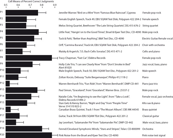
Figure 3.15The ability of different kinds of program to reveal spectral errors in reproduced sound.
From data in Olive (1994).
Figure 3.16 shows that an important requirement for good program material is a long-term spectrum that well represents most of the audible frequencies, presumably giving listeners more opportunity to judge. What they were judging in these tests was the ability to hear narrow and broadband spectral variations in loudspeakers, arguably the problems most disruptive of sound quality/timbre.
The inversion of the bass contents of Groups 3 and 4 breaks what seems like a trend, indicating that there is more to this than long-term spectral content. Vocal/instrumental composition is another factor, some of which can be seen in the program listings in Figure 3.15. And, finally, there is the inescapable factor of the “circle of confusion”—we don’t know what spectral irregularities are incorporated into the recordings. More specific details are in Olive (1994).
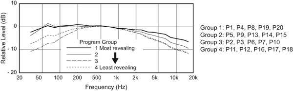
From Olive (1994).
Clearly there are no hard rules but, in general, complex productions with broadband, relatively constant spectra aid listeners in finding problems. The notion that “acoustical,” especially classical, music has inherent superiority was not supported. Solo instruments and voices appear not to be very helpful, however comfortable we may feel with them. A variety of programs should be used. Amusingly, a program that is good for demonstrations (e.g., selling) can be different from that which is needed for evaluation (e.g., buying).
The maturity of this technology means that problems with linear or non-linear distortions in the signal path are normally not expected. However, they happen, so some simple tests are in order. It is essential to confirm that the power amplifier(s) being used are operating within their designed operating ranges. Power amplifiers must have very low output impedances (high damping factor), otherwise they will cause changes to the frequency responses of the loudspeakers (see Chapter 16). This eliminates almost all vacuum-tube and some lesser class-D power amplifiers, although high-quality ones are fine. Class AB power amplifiers are a safe choice. Non-linearities in competently designed amplifiers are insignificant to the outcome of loudspeaker evaluations, so long as voltage or current limiting and overload protection are avoided. It is wise to measure the frequency-dependent impedances of loudspeakers under test to ensure that they do not drop below values that the amplifiers can safely drive. Some of these requirements will be difficult to find for many amplifiers as they are not always specified. Adequately sized speaker wire (Chapter 16) and audio frequency analog interconnects are transparent—in spite of advertising and folklore to the contrary. Digital communication and interfacing is a different and increasingly complex matter—and outside my comfort zone to discuss.
This is the primary reason for blind tests. Section 3.1 shows persuasive evidence that humans are notoriously easy to bias with foreknowledge of what they are listening to. An acoustically transparent screen is a remarkable device for revealing the truth about what is or is not audible.
The efficiency and effectiveness of listening tests improves as listeners learn which aspects of a performance to listen for during different portions of familiar programs. Select a number of short excerpts from music known to be revealing, and use them repeatedly in prerecorded randomized sequences. They can be edited and assembled on computers. It is not entertainment, but the selections must have some musical merit or they will be annoying. After many, many repetitions the music becomes just a test signal, but because of the familiarity, it is extremely informative. Because the circle of confusion is a reality, it is essential to use several selections from different sources, recording engineers, labels and so forth. By paying attention, it will soon become clear which selections are helpful and which are just taking up time. Ask your listeners what they use to form their opinions. It has been known for listeners to have a very narrow focus—like using only the kick drum, or ignoring anything classical, or ignoring anything popular, or listening only to voices. Such listeners should not be invited back. It is also not uncommon for the peculiarities of certain programs to be adapted to. For example, one pop/rock excerpt that was very revealing of spectral features was expected to have slightly too much low bass; others might be known to be slightly bright. All of this relates to the circle of confusion, but these characteristics can recognized and accepted only when auditioned in the company of several other musical selections.
We adapt to the space we are in and appear to be able to “listen through” it to discern qualities about the source that would otherwise be masked. It takes time to acquire that ability, so schedule a warm-up session before serious listening begins or discard the results from early rounds.
For most people, critical listening of this intensity is a first-time experience. They may feel unprepared for it and are anxious. For audiophiles with opinions, pride is involved, leading to a different kind of tension. Seeing some preliminary test results showing that their opinions are not random is very confidence inspiring. This is the normal situation unless serious hearing loss is involved. Don’t place much importance on the results of the first few test sessions. However, most listeners settle in quickly, and become quite comfortable with the circumstances. Experienced listeners are operational immediately, and some actually enjoy it—I did.
Not all of us are good listeners, just as not all of us can dance or sing well. If one is establishing a population of listeners from which to draw over the long term, it will be necessary to monitor their decisions, looking for those who (a) exhibit small variations in repeated judgments and (b) differentiate their opinions of products by using a large numerical range of ratings (Toole, 1985; Olive, 2001, 2003). An interesting side note to this is that the interests, experience and, indeed, occupations of listeners are factors. Musicians have long been assumed to have superior abilities to judge sound quality. Certainly, they know music, and they tend to be able to articulate opinions about sound. But, what about the opinions themselves? Does living “in the band” develop an ability to judge sound from the audience’s perspective? Does understanding the structure of music and how it should be played enable a superior analysis of sound quality? When put to the test, Gabrielsson and Sjögren (1979) found that the listeners who were the most reliable and also the most observant of differences between test sounds were persons he identified as hi-fi enthusiasts, a population that also included some musicians. The worst were those who had no hi-fi interests. In the middle were musicians who were not hi-fi-oriented. This corresponds with the author’s own observations over many years.
Perhaps the most detailed analysis of listener abilities was in an EIA-J (Electronic Industries Association of Japan) document (EIA-J, 1979), which is shown in Figure 3.17. It is not known how much statistical rigor was applied to the analysis of listener performance, but it was the result of several years of observation and a very large number of listening tests (personal communication from a committee member).
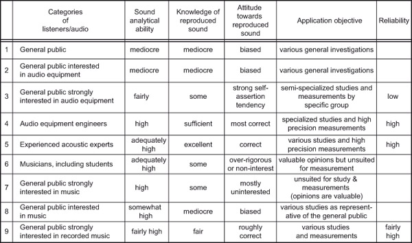
From EIA-J, 1979.
Olive (2003) analyzed the opinions of 268 listeners who participated in evaluations of the same four loudspeakers. Twelve of those listeners had been selected and trained and had participated in numerous double-blind listening tests. The others were visitors to the Harman International research lab, as a part of dealer or distributor training or in promotional tours. The results shown earlier in Figure 3.9 reveal that the trained, veteran listeners distinguished themselves by having the highest performance rating by far, but obviously years of experience selling and listening on store floors has had a positive effect on the retail sales personnel.
Olive (1994) describes the listener training process, which is also a part of the selection process; those lacking the aptitude do not improve beyond a moderate level. It teaches listeners to recognize and describe resonances, the most common defect in loudspeakers. It does not train them to recognize any specific “voicing,” as some have suspected. Instead, by a process of eliminating timbre-modifying resonances, the preferences gravitate to “neutral” loudspeakers, through which listeners get to hear the unmodified recordings.
It is common to think that persons from different countries or cultures might prefer certain spectral balances. It is also common to think that people of different ages, having grown up with different music might have preferences that are not shared by young people. Harman is a large international company, with audio business in all product categories—consumer, professional and automotive—so it is important to know if such biases exist, and if they do, to be able to design products that appeal to specific clienteles. Over the years several investigations have shown that, if such biases exist at all, they are not revealed in blind testing. Figure 3.1 shows two “voicings” of the same loudspeaker, one done by the Danish design team and another by a consultant hired by the German distributor to modify the product to fit the expectations of his clients. The two versions were very similar in sound, and after extended double-blind listening by an international listener pool, including Germans, there was no evidence of a significant preference. Olive has conducted numerous sound quality evaluations with listeners from Europe, Canada, Japan and China, and has yet to find any evidence of cultural bias. Figure 3.18 shows the result for headphone evaluations. Similar results have been found for loudspeakers and car audio. The same is true with respect of age—except, as shown in Figure 3.7, older listeners tend to exhibit greater variation in their opinions because of degraded hearing.
Section 3.2 has shown that there are significant detrimental effects of hearing loss. Audiometric thresholds within about 20 dB of normal are desirable.
Listeners in groups are sometimes observed to vote as a group, following the body language, subtle noises, or verbalizations of one of the number who is judged to be the most likely to “know.” For this reason, controlled tests should be done with a single listener, but this is not always possible. In such cases, firm instructions must be issued to avoid all verbal and non-verbal communication. Opinionated persons and self-appointed gurus tend to want to “share” by any means possible. Video surveillance is a deterrent.
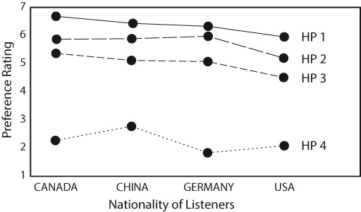
From Olive et al. (2014).
The premise of controlled listening tests is that each new sound presentation will be judged in the same context as all others. This theoretical ideal sometimes goes astray when one or more products in a group being evaluated exhibit features that are distinctive enough to be recognized. This may or may not alter the rating given to the product, but it surely will affect the variations in that rating that would normally occur. If listeners are aware of the products in the test group, even though they are presented “blind,” it is almost inevitable that they will attempt to guess the identities. The test is no longer a fair and balanced assessment. For this reason it is good practice to add one or more “unknowns” to the test population and to let that fact be known in an attempt to preclude a distracting guessing game.
Most people realize that the way a test is conducted can affect its outcome. That is why we do double-blind tests—one “blind” is for the listeners, so they don’t know what they are listening to; the second “blind” is to prevent the experimenter from influencing the outcome of the test.
The simplest of all tests, and a method much used by product reviewers, is the “take-it-home-and-listen-to-it,” or single-stimulus, method. In addition to being “sighted,” and therefore subject to all possible non-auditory influences, it allows for adaptation. Humans are superb at normalizing many otherwise audible factors. This means that characteristics that might be perceived as virtues or flaws in a different kind of test can go unnoticed.
The scientific method prefers more controls, fewer opportunities for non-auditory factors to influence an auditory decision. It is what we hear that matters, not what we think we hear. Critics complain that rapid comparisons don’t allow enough time for listeners to settle into a comfort zone within which small problems might become apparent. Of course, a time limit is not a requirement for a controlled test. It could go on for days. Listeners can listen to any of the optional sounds whenever they like. All that is required is that the listeners remain ignorant of the identity of the products—and that seems to be the principal problem for many reviewers.
Having followed subjective reviews for many years, in several well-known magazines and webzines, I find myself being amazed at how much praise is heaped on products that by any rational subjective or objective evaluation would be classified as significantly flawed. No, the single-stimulus, take-it-home-and-listen-to-it method is at best excusable as an expedient solution for budget and/or time-constrained reviewers. At worst it is a “feel-good” palliative for the reviewer. At no time is it a test procedure for generating useful guidance for readers.
A simple A versus B paired comparison is an important step in the right direction. The problem with a solitary paired comparison is that problems shared by both products may not be noticed. There is evidence that in such a comparison the first and second sounds in the sequence are not treated equally, so it is necessary to randomly mix A-B and B-A presentations, and always to disguise the identities.
Several paired comparisons among more than two products selected and presented in randomized order is a much better method, but it is very time-consuming. If a computer is not used for randomization in real time, it is possible to generate a randomized presentation schedule in advance and follow it.
A multiple comparison with three or four products simultaneously available for comparison is how I conducted my very first listening tests, back in the 1960s, and it is still the preferred method. It is efficient, highly repeatable, and provides listeners with an opportunity to separate the variables: the loudspeaker, the room and the program. If positional substitution is not used, remember to randomize the locations of the loudspeakers between musical selections.
In addition, there are important issues of what questions to ask the listeners, scaling the results, statistical analysis and so on. It has become a science unto itself. (See Toole and Olive, 2001; Bech and Zacharov, 2006, for elaborations of experimental procedures and statistical analysis of results.) However, as has been found, even rudimentary experimental controls and elementary statistics can take one a long way.
These tests have been criticized for many reasons, and I would like to think that all have been satisfactorily put to rest. Perhaps the most persistent challenge is the belief that as long as the term “preference” is involved, the results merely reflect the likes, dislikes and tastes of an inexpert audience, not the analytical criticism of listeners who know what good sound really is. They assert that the objective should be “realism,” “accuracy,” “fidelity,” “truth” and the like.
As it turns out, this is where my investigations started, many years ago. I required listeners to report their summary opinions, their “Gestalt,” as a number on a 0 to 10 “Fidelity” scale. The number 10 represented the most perfect sound they can recall, and 0 was unrecognizable rubbish. When these tests began, it is fair to say that some of the loudspeakers approached “rubbish” and none came close to perfection. Consequently, scores extended over a significant range. To help listeners retain an impression of what constituted good and bad sound, the Fidelity scale was anchored by always including in the population of test loudspeakers at least one that was at the low end of the scale and one that was at the high end, usually the one we dubbed the “king of the hill,” the best of the test population to that date. A parallel scale was provided, called “preference,” thinking that there might be a difference, but the two ratings “fidelity” and “preference” simply tracked each other.
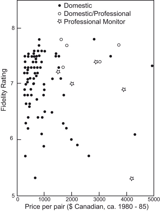
Figure 3.19 illustrates the cumulative results from our NRCC tests in the early 1980s—a slice of the history of audio. It is obvious that there are many loudspeakers clustered near the top of the scale. As time passed more products were rated highly, and listeners complained about wasting time listening to bad sound. I stopped anchoring the scale at the low end, and an interesting thing happened: most listeners continued to use the same numerical range to describe what they heard. The scores rarely went above 8, which is a common subjective scaling phenomenon—people like to leave some “headroom” in case something better comes along. The advantage was that it was now easier to distinguish the rankings of the remaining loudspeakers because they were more widely separated on the scale. However, it was evident that they were no longer judging on the same scale—the upper end of it had stretched. When listening to just a few of the top-rated loudspeakers, which in Figure 3.19 would have been crowded together, statistically difficult to separate, the same product ratings would cover a much larger portion of the scale and be easy to separate and rank. Listeners were still judging fidelity, but it was rated on an elastic scale. I chose to call it preference, and it still is.
Listeners obviously have a “preference” for high “fidelity,” also known as “accuracy,” “realism” and so on. It is really one scale.
Figure 3.19 is somewhat provocative in that it shows inexpensive loudspeakers being competitive with much more expensive ones. At moderate sound levels that can be true, especially if one is willing to accept limited bass extension. But most of the small inexpensive products misbehave at high sound levels, and almost certainly they do not have the compelling industrial design and exotic finishes that more expensive products have. It is possible to see a slight upward step in the ratings around $1,000 per pair, when the price could justify a woofer in a floor-standing product. The dedicated professional monitor loudspeakers in these tests had some problems. Over the years everything has improved from these examples, and the best of today’s products would surpass all of the products in these tests, although poor ones persist.