Chapter 8. Unsupervised Methods: Topic Modeling and Clustering
When working with a large number of documents, one of the first questions you want to ask without reading all of them is “What are they talking about?” You are interested in the general topics of the documents, i.e., which (ideally semantic) words are often used together.
Topic modeling tries to solve that challenge by using statistical techniques for finding out topics from a corpus of documents. Depending on your vectorization (see Chapter 5), you might find different kinds of topics. Topics consist of a probability distribution of features (words, n-grams, etc.).
Topics normally overlap with each other; they are not clearly separated. The same is true for documents: it is not possible to assign a document uniquely to a single topic; a document always contains a mixture of different topics. The aim of topic modeling is not primarily to assign a topic to an arbitrary document but to find the global structure of the corpus.
Often, a set of documents has an explicit structure that is given by categories, keywords, and so on. If we want to take a look at the organic composition of the corpus, then topic modeling will help a lot to uncover the latent structure.
Topic modeling has been known for a long time and has gained immense popularity during the last 15 years, mainly due to the invention of LDA,1 a stochastic method for discovering topics. LDA is flexible and allows many modifications. However, it is not the only method for topic modeling (although you might believe this by looking at the literature, much of which is biased toward LDA). Conceptually simpler methods are non-negative matrix factorization, singular-value decomposition (sometimes called LSI), and a few others.
What You’ll Learn and What We’ll Build
In this chapter, we will take an in-depth look at the various methods of topic modeling, try to find differences and similarities between the methods, and run them on the same use case. Depending on your requirements, it might also be a good idea to not only try a single method but compare the results of a few.
After studying this chapter, you will know the different methods of topic modeling and their specific advantages and drawbacks. You will understand how topic modeling can be applied not only to find topics but also to create quick summaries of document corpora. You will learn about the importance of choosing the correct granularity of entities for calculating topic models. You have experimented with many parameters to find the optimal topic model. You are able to judge the quality of the resulting topic models by quantitative methods and numbers.
Our Dataset: UN General Debates
Our use case is to semantically analyze the corpus of the UN general debates. You might know this dataset from the earlier chapter about text statistics.
This time we are more interested in the meaning and in the semantic content of the speeches and how we can arrange them topically. We want to know what the speakers are talking about and answer questions like these: Is there a structure in the document corpus? What are the topics? Which of them is most prominent? Does this change over time?
Checking Statistics of the Corpus
Before starting with topic modeling, it is always a good idea to check the statistics of the underlying text corpus. Depending on the results of this analysis, you will often choose to analyze different entities, e.g., documents, sections, or paragraphs of text.
We are not so much interested in authors and additional information, so it’s enough to work with one of the supplied CSV files:
importpandasaspddebates=pd.read_csv("un-general-debates.csv")debates.info()
Out:
<class'pandas.core.frame.DataFrame'>RangeIndex:7507entries,0to7506Datacolumns(total4columns):session7507non-nullint64year7507non-nullint64country7507non-nullobjecttext7507non-nullobjectdtypes:int64(2),object(2)memoryusage:234.7+KB
The result looks fine. There are no null values in the text column; we might use years and countries later, and they also have only non-null values.
The speeches are quite long and cover a lot of topics as each country is allowed only to deliver a single speech per year. Different parts of the speeches are almost always separated by paragraphs. Unfortunately, the dataset has some formatting issues. Compare the text of two selected speeches:
(repr(df.iloc[2666]["text"][0:200]))(repr(df.iloc[4729]["text"][0:200]))
Out:
'\ufeffIt is indeed a pleasure for me and the members of my delegation to
extend to Ambassador Garba our sincere congratulations on his election to the
presidency of the forty-fourth session of the General '
'\ufeffOn behalf of the State of Kuwait, it\ngives me pleasure to congratulate
Mr. Han Seung-soo,\nand his friendly country, the Republic of Korea, on
his\nelection as President of the fifty-sixth session of t'
As you can see, in some speeches the newline character is used to separate paragraphs. In the transcription of other speeches, a newline is used to separate lines. To recover the paragraphs, we therefore cannot just split at newlines. It turns out that splitting at stops, exclamation points, or question marks occurring at line ends works well enough. We ignore spaces after the stops:
importredf["paragraphs"]=df["text"].map(lambdatext:re.split('[.?!]\s*\n',text))df["number_of_paragraphs"]=df["paragraphs"].map(len)
From the analysis in Chapter 2, we already know that the number of speeches per year does not change much. Is this also true for the number of paragraphs?
%matplotlibinlinedebates.groupby('year').agg({'number_of_paragraphs':'mean'}).plot.bar()
Out:

The average number of paragraphs has dropped considerably over time. We would have expected that, as the number of speakers per year increased and the total time for speeches is limited.
Apart from that, the statistical analysis shows no systematic problems with the dataset. The corpus is still quite up-to-date; there is no missing data for any year. We can now safely start with uncovering the latent structure and detect topics.
Preparations
Topic modeling is a machine learning method and needs vectorized data. All topic modeling methods start with the document-term matrix. Recalling the meaning of this matrix (which was introduced in Chapter 4), its elements are word frequencies (or often scaled as TF-IDF weights) of the words (columns) in the corresponding documents (rows). The matrix is sparse, as most documents contain only a small fraction of the vocabulary.
Let’s calculate the TF-IDF matrix both for the speeches and for the paragraphs of the speeches. First, we have to import the necessary packages from scikit-learn. We start with a naive approach and use the standard spaCy stop words:
fromsklearn.feature_extraction.textimportTfidfVectorizerfromspacy.lang.en.stop_wordsimportSTOP_WORDSasstopwords
Calculating the document-term matrix for the speeches is easy; we also include bigrams:
tfidf_text=TfidfVectorizer(stop_words=stopwords,min_df=5,max_df=0.7)vectors_text=tfidf_text.fit_transform(debates['text'])vectors_text.shape
Out:
(7507, 24611)
For the paragraphs, it’s a bit more complicated as we have to flatten the list first. In the same step, we omit empty paragraphs:
# flatten the paragraphs keeping the yearsparagraph_df=pd.DataFrame([{"text":paragraph,"year":year}forparagraphs,yearin\zip(df["paragraphs"],df["year"])forparagraphinparagraphsifparagraph])tfidf_para_vectorizer=TfidfVectorizer(stop_words=stopwords,min_df=5,max_df=0.7)tfidf_para_vectors=tfidf_para_vectorizer.fit_transform(paragraph_df["text"])tfidf_para_vectors.shape
Out:
(282210, 25165)
Of course, the paragraph matrix has many more rows. The number of columns (words) is also different because min_df and max_df have an effect in selecting features, as the number of documents has changed.
Nonnegative Matrix Factorization (NMF)
The conceptually easiest way to find a latent structure in the document corpus is the factorization of the document-term matrix. Fortunately, the document-term matrix has only positive-value elements; therefore, we can use methods from linear algebra that allow us to represent the matrix as the product of two other nonnegative matrices. Conventionally, the original matrix is called V, and the factors are W and H:
Or we can represent it graphically (visualizing the dimensions necessary for matrix multiplication), as in Figure 8-1.
Depending on the dimensions, the factorization can be performed exactly. But as this is so much more computationally expensive, an approximate factorization is sufficient.

Figure 8-1. Schematic nonnegative matrix factorization; the original matrix V is decomposed into W and H.
In the context of text analytics, both W and H have an interpretation. The matrix W has the same number of rows as the document-term matrix and therefore maps documents to topics (document-topic matrix). H has the same number of columns as features, so it shows how the topics are constituted of features (topic-feature matrix). The number of topics (the columns of W and the rows of H) can be chosen arbitrarily. The smaller this number, the less exact the factorization.
Blueprint: Creating a Topic Model Using NMF for Documents
It’s really easy to perform this decomposition for speeches in scikit-learn. As (almost) all topic models need the number of topics as a parameter, we arbitrarily choose 10 topics (which will later turn out to be a good choice):
fromsklearn.decompositionimportNMFnmf_text_model=NMF(n_components=10,random_state=42)W_text_matrix=nmf_text_model.fit_transform(tfidf_text_vectors)H_text_matrix=nmf_text_model.components_
Similar to the TfidfVectorizer, NMF also has a fit_transform method that returns one of the positive factor matrices. The other factor can be accessed by the components_ member variable of the NMF class.
Topics are word distributions. We are now going to analyze this distribution and see whether we can find an interpretation of the topics. Taking a look at Figure 8-1, we need to consider the H matrix and find the index of the largest values in each row (topic) that we then use as a lookup index in the vocabulary. As this is helpful for all topic models, we define a function for outputting a summary:
defdisplay_topics(model,features,no_top_words=5):fortopic,word_vectorinenumerate(model.components_):total=word_vector.sum()largest=word_vector.argsort()[::-1]# invert sort order("\nTopic%02d"%topic)foriinrange(0,no_top_words):("%s(%2.2f)"%(features[largest[i]],word_vector[largest[i]]*100.0/total))
Calling this function, we get a nice summary of the topics that NMF detected in the speeches (the numbers are the percentage contributions of the words to the respective topic):
display_topics(nmf_text_model,tfidf_text_vectorizer.get_feature_names())
Out:
| Topic 00 co (0.79) operation (0.65) disarmament (0.36) nuclear (0.34) relations (0.25) |
Topic 01 terrorism (0.38) challenges (0.32) sustainable (0.30) millennium (0.29) reform (0.28) |
Topic 02 africa (1.15) african (0.82) south (0.63) namibia (0.36) delegation (0.30) |
Topic 03 arab (1.02) israel (0.89) palestinian (0.60) lebanon (0.54) israeli (0.54) |
Topic 04 american (0.33) america (0.31) latin (0.31) panama (0.21) bolivia (0.21) |
| Topic 05 pacific (1.55) islands (1.23) solomon (0.86) island (0.82) fiji (0.71) |
Topic 06 soviet (0.81) republic (0.78) nuclear (0.68) viet (0.64) socialist (0.63) |
Topic 07 guinea (4.26) equatorial (1.75) bissau (1.53) papua (1.47) republic (0.57) |
Topic 08 european (0.61) europe (0.44) cooperation (0.39) bosnia (0.34) herzegovina (0.30) |
Topic 09 caribbean (0.98) small (0.66) bahamas (0.63) saint (0.63) barbados (0.61) |
Topic 00 and Topic 01 look really promising as people are talking about nuclear disarmament and terrorism. These are definitely real topics in the UN general debates.
The subsequent topics, however, are more or less focused on different regions of the world. This is due to speakers mentioning primarily their own country and neighboring countries. This is especially evident in Topic 03, which reflects the conflict in the Middle East.
It’s also interesting to take a look at the percentages with which the words contribute to the topics. Due to the large number of words, the individual contributions are quite small, except for guinea in Topic 07. As we will see later, the percentages of the words within a topic are a good indication for the quality of the topic model. If the percentage within a topic is rapidly decreasing, the topic is well-defined, whereas slowly decreasing word probabilities indicate a less-pronounced topic. It’s much more difficult to intuitively find out how well the topics are separated; we will take a look at that later.
It would be interesting to find out how “big” the topics are, i.e., how many documents could be assigned mainly to each topic. This can be calculated using the document-topic matrix and summing the individual topic contributions over all documents. Normalizing them with the total sum and multiplying by 100 gives a percentage value:
W_text_matrix.sum(axis=0)/W_text_matrix.sum()*100.0
Out:
array([11.13926287,17.07197914,13.64509781,10.18184685,11.43081404,5.94072639,7.89602474,4.17282682,11.83871081,6.68271054])
We can easily see that there are smaller and larger topics but basically no outliers. Having an even distribution is a quality indicator. If your topic models have, for example, one or two large topics compared to all the others, you should probably adjust the number of topics.
In the next section, we will use the paragraphs of the speeches as entities for topic modeling and try to find out if that improves the topics.
Blueprint: Creating a Topic Model for Paragraphs Using NMF
In UN general debates, as in many other texts, different topics are often mixed, and it is hard for the topic modeling algorithm to find a common topic of an individual speech. Especially in longer texts, it happens quite often that documents do not cover just one but several topics. How can we deal with that? One idea is to find smaller entities in the documents that are more coherent from a topic perspective.
In our corpus, paragraphs are a natural subdivision of speeches, and we can assume that the speakers try to stick to one topic within one paragraph. In many documents, paragraphs are a good candidate (if they can be identified as such), and we have already prepared the corresponding TF-IDF vectors. Let’s try to calculate their topic models:
nmf_para_model=NMF(n_components=10,random_state=42)W_para_matrix=nmf_para_model.fit_transform(tfidf_para_vectors)H_para_matrix=nmf_para_model.components_
Our display_topics function developed earlier can be used to find the content of the topics:
display_topics(nmf_para_model,tfidf_para_vectorizer.get_feature_names())
Out:
| Topic 00 nations (5.63) united (5.52) organization (1.27) states (1.03) charter (0.93) |
Topic 01 general (2.87) session (2.83) assembly (2.81) mr (1.98) president (1.81) |
Topic 02 countries (4.44) developing (2.49) economic (1.49) developed (1.35) trade (0.92) |
Topic 03 people (1.36) peace (1.34) east (1.28) middle (1.17) palestinian (1.14) |
Topic 04 nuclear (4.93) weapons (3.27) disarmament (2.01) treaty (1.70) proliferation (1.46) |
| Topic 05 rights (6.49) human (6.18) respect (1.15) fundamental (0.86) universal (0.82) |
Topic 06 africa (3.83) south (3.32) african (1.70) namibia (1.38) apartheid (1.19) |
Topic 07 security (6.13) council (5.88) permanent (1.50) reform (1.48) peace (1.30) |
Topic 08 international (2.05) world (1.50) community (0.92) new (0.77) peace (0.67) |
Topic 09 development (4.47) sustainable (1.18) economic (1.07) social (1.00) goals (0.93) |
Compared to the previous results for topic modeling speeches, we have almost lost all countries or regions except for South Africa and the Middle East. These are due to the regional conflicts that sparked interest in other parts of the world. Topics in the paragraphs like “Human rights,” “international relations,” “developing countries,” “nuclear weapons,” “security council,” “world peace,” and “sustainable development” (the last one probably occurring only lately) look much more reasonable compared to the topics of the speeches. Taking a look at the percentage values of the words, we can observe that they are dropping much faster, and the topics are more pronounced.
Latent Semantic Analysis/Indexing
Another algorithm for performing topic modeling is based on the so-called singular value decomposition (SVD), another method from linear algebra.
Graphically, it is possible to conceive SVD as rearranging documents and words in a way to uncover a block structure in the document-term matrix. There is a nice visualization of that process at topicmodels.info. Figure 8-2 shows the start of the document-term matrix and the resulting block diagonal form.
Making use of the principal axis theorem, orthogonal n × n matrices have an eigenvalue decomposition. Unfortunately, we do not have orthogonal square document-term matrices (except for rare cases). Therefore, we need a generalization called singular value decomposition. In its most general form, the theorem states that any m × n matrix V can be decomposed as follows:
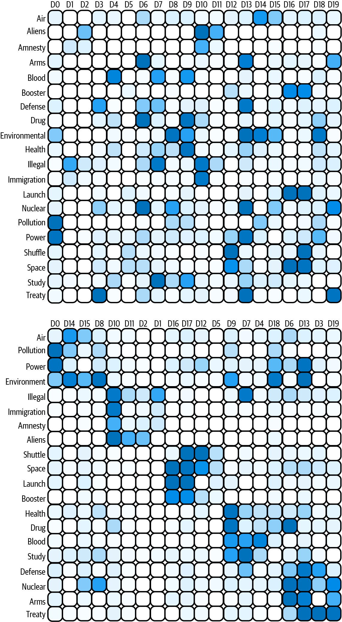
Figure 8-2. Visualization of topic modeling with SVD.
U is a unitary m × m matrix, V* is an n × n matrix, and Σ is an m × n diagonal matrix containing the singular values. There are exact solutions for this equation, but as they take a lot of time and computational effort to find, we are looking for approximate solutions that can be found quickly. The approximation works by only considering the largest singular values. This leads to Σ becoming a t × t matrix; in turn, U has m × t and V* t × n dimensions. Graphically, this is similar to the nonnegative matrix factorization, as shown in Figure 8-3.
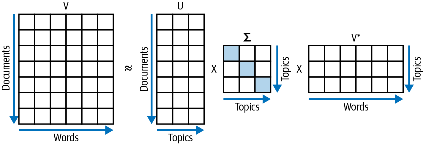
Figure 8-3. Schematic singular value decomposition.
The singular values are the diagonal elements of Σ. The document-topic relations are included in U, whereas the word-to-topic mapping is represented by V*. Note that neither the elements of U nor the elements of V* are guaranteed to be positive. The relative sizes of the contributions will still be interpretable, but the probability explanation is no longer valid.
Blueprint: Creating a Topic Model for Paragraphs with SVD
In scikit-learn the interface to SVD is identical to that of NMF. This time we start directly with the paragraphs:
fromsklearn.decompositionimportTruncatedSVDsvd_para_model=TruncatedSVD(n_components=10,random_state=42)W_svd_para_matrix=svd_para_model.fit_transform(tfidf_para_vectors)H_svd_para_matrix=svd_para_model.components_
Our previously defined function for evaluating the topic model can also be used:
display_topics(svd_para_model,tfidf_para_vectorizer.get_feature_names())
Out:
| Topic 00 nations (0.67) united (0.65) international (0.58) peace (0.46) world (0.46) |
Topic 01 general (14.04) assembly (13.09) session (12.94) mr (10.02) president (8.59) |
Topic 02 countries (19.15) development (14.61) economic (13.91) developing (13.00) session (10.29) |
Topic 03 nations (4.41) united (4.06) development (0.95) organization (0.84) charter (0.80) |
Topic 04 nuclear (21.13) weapons (14.01) disarmament (9.02) treaty (7.23) proliferation (6.31) |
| Topic 05 rights (29.50) human (28.81) nuclear (9.20) weapons (6.42) respect (4.98) |
Topic 06 africa (8.73) south (8.24) united (3.91) african (3.71) nations (3.41) |
Topic 07 council (14.96) security (13.38) africa (8.50) south (6.11) african (3.94) |
Topic 08 world (48.49) international (41.03) peace (32.98) community (23.27) africa (22.00) |
Topic 09 development (63.98) sustainable (20.78) peace (20.74) goals (15.92) africa (15.61) |
Most of the resulting topics are surprisingly similar to those of the nonnegative matrix factorization. However, the Middle East conflict does not appear as a separate topic this time. As the topic-word mappings can also have negative values, the normalization varies from topic to topic. Only the relative sizes of the words constituting the topics are relevant.
Don’t worry about the negative percentages. These arise as SVD does not guarantee positive values in W, so contributions of individual words might be negative. This means that words appearing in documents “reject” the corresponding topic.
If we want to determine the sizes of the topics, we now have to take a look at the singular values of the decomposition:
svd_para.singular_values_
Out:
array([68.21400653,39.20120165,36.36831431,33.44682727,31.76183677,30.59557993,29.14061799,27.40264054,26.85684195,25.90408013])
The sizes of the topics also correspond quite nicely with the ones from the NMF method for the paragraphs.
Both NMF and SVF have used the document-term matrix (with TF-IDF transformations applied) as a basis for the topic decomposition. Also, the dimensions of the U matrix are identical to those of W; the same is true for V* and H. It is therefore not surprising that both of these methods produce similar and comparable results. As these methods are really fast to calculate, for real-life projects we recommend starting with the linear algebra methods.
We will now turn away from these linear-algebra-based methods and focus on probabilistic topic models, which have become immensely popular in the past 20 years.
Latent Dirichlet Allocation
LDA is arguably the most prominent method of topic modeling in use today. It has been popularized during the last 15 years and can be adapted in flexible ways to different usage scenarios.
How does it work?
LDA views each document as consisting of different topics. In other words, each document is a mix of different topics. In the same way, topics are mixed from words. To keep the number of topics per document low and to have only a few, important words constituting the topics, LDA initially uses a Dirichlet distribution, a so-called Dirichlet prior. This is applied both for assigning topics to documents and for finding words for the topics. The Dirichlet distribution ensures that documents have only a small number of topics and topics are mainly defined by a small number of words. Assuming that LDA generated topic distributions like the previous ones, a topic could be made up of words like nuclear, treaty, and disarmament, while another topic would be sampled by sustainable, development, etc.
After the initial assignments, the generative process starts. It uses the Dirichlet distributions for topics and words and tries to re-create the words from the original documents with stochastic sampling. This process has to be iterated many times and is therefore computationally intensive.2 On the other hand, the results can be used to generate documents for any identified topic.
Blueprint: Creating a Topic Model for Paragraphs with LDA
Scikit-learn hides all these differences and uses the same API as the other topic modeling methods:
fromsklearn.feature_extraction.textimportCountVectorizercount_para_vectorizer=CountVectorizer(stop_words=stopwords,min_df=5,max_df=0.7)count_para_vectors=count_para_vectorizer.fit_transform(paragraph_df["text"])
fromsklearn.decompositionimportLatentDirichletAllocationlda_para_model=LatentDirichletAllocation(n_components=10,random_state=42)W_lda_para_matrix=lda_para_model.fit_transform(count_para_vectors)H_lda_para_matrix=lda_para_model.components_
Waiting Time
Due to the probabilistic sampling, the process takes a lot longer than NMF and SVD. Expect at least minutes, if not hours, of runtime.
Our utility function can again be used to visualize the latent topics of the paragraph corpus:
display_topics(lda_para_model,tfidf_para.get_feature_names())
Out:
| Topic 00 africa (2.38) people (1.86) south (1.57) namibia (0.88) regime (0.75) |
Topic 01 republic (1.52) government (1.39) united (1.21) peace (1.16) people (1.02) |
Topic 02 general (4.22) assembly (3.63) session (3.38) president (2.33) mr (2.32) |
Topic 03 human (3.62) rights (3.48) international (1.83) law (1.01) terrorism (0.99) |
Topic 04 world (2.22) people (1.14) countries (0.94) years (0.88) today (0.66) |
| Topic 05 peace (1.76) security (1.63) east (1.34) middle (1.34) israel (1.24) |
Topic 06 countries (3.19) development (2.70) economic (2.22) developing (1.61) international (1.45) |
Topic 07 nuclear (3.14) weapons (2.32) disarmament (1.82) states (1.47) arms (1.46) |
Topic 08 nations (5.50) united (5.11) international (1.46) security (1.45) organization (1.44) |
Topic 09 international (1.96) world (1.91) peace (1.60) economic (1.00) relations (0.99) |
It’s interesting to observe that LDA has generated a completely different topic structure compared to the linear algebra methods described earlier. People is the most prominent word in three quite different topics. In Topic 04, South Africa is related to Israel and Palestine, while in Topic 00, Cyprus, Afghanistan, and Iraq are related. This is not easy to explain. This is also reflected in the slowly decreasing word weights of the topics.
Other topics are easier to comprehend, such as climate change, nuclear weapons, elections, developing countries, and organizational questions.
In this example, LDA does not yield much better results than either NMF or SVD. However, due to the sampling process, LDA is not limited to sample topics just consisting of words. There are several variations, such as author-topic models, that can also sample categorical features. Moreover, as there is so much research going on in LDA, other ideas are published quite frequently, which extend the focus of the method well beyond text analytics (see, for example, Minghui Qiu et al., “It Is Not Just What We Say, But How We Say Them: LDA-based Behavior-Topic Model” or Rahji Abdurehman, “Keyword-Assisted LDA: Exploring New Methods for Supervised Topic Modeling”).
Blueprint: Visualizing LDA Results
As LDA is so popular, there is a nice package in Python to visualize the LDA results called pyLDAvis.3 Fortunately, it can directly use the results from sciki-learn for its visualization.
Be careful, this takes some time:
importpyLDAvis.sklearnlda_display=pyLDAvis.sklearn.prepare(lda_para_model,count_para_vectors,count_para_vectorizer,sort_topics=False)pyLDAvis.display(lda_display)
Out:
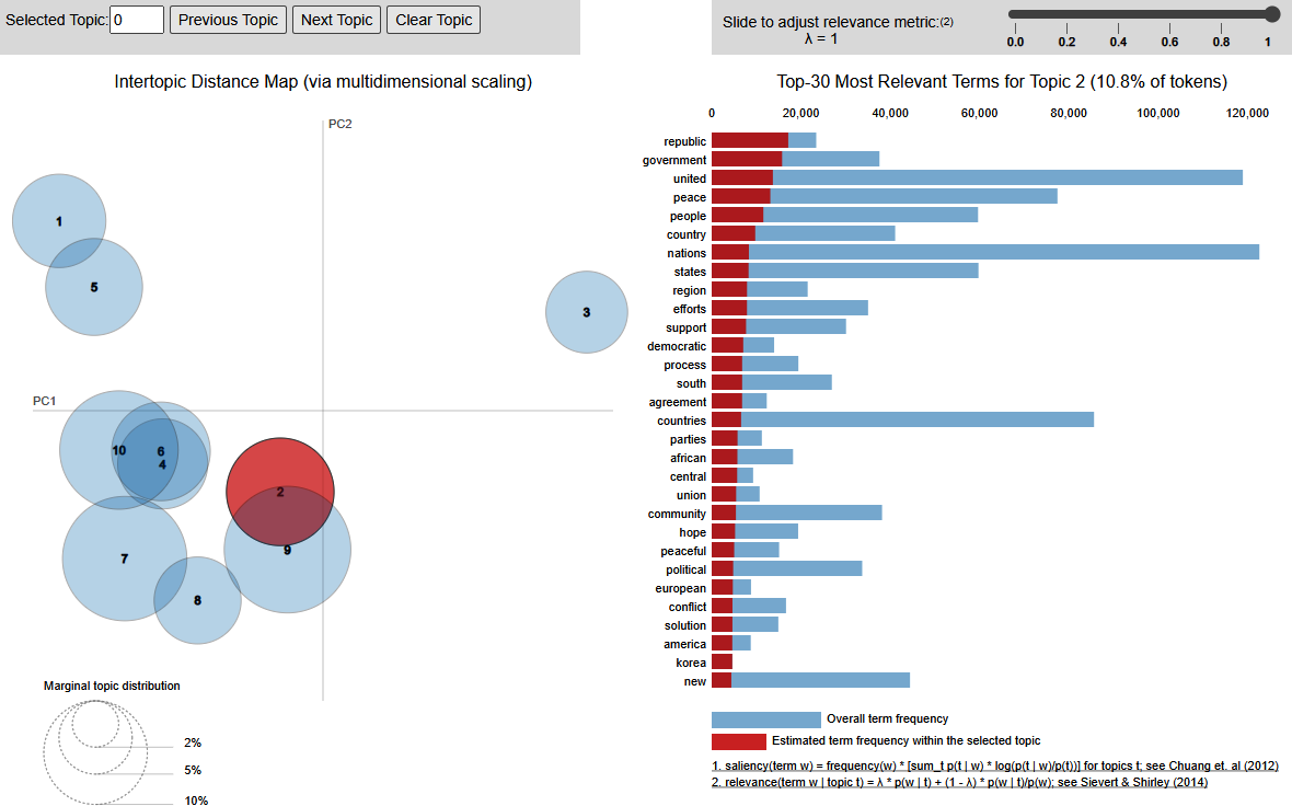
There is a multitude of information available in the visualization. Let’s start with the topic “bubbles” and click the topic. Now take a look at the red bars, which symbolize the word distribution in the currently selected topic. As the length of the bars is not decreasing quickly, Topic 2 is not very pronounced. This is the same effect you can see in the table from “Blueprint: Creating a Topic Model for Paragraphs with LDA” (look at Topic 1, where we have used the array indices, whereas pyLDAvis starts enumerating the topics with 1).
To visualize the results, the topics are mapped from their original dimension (the number of words) into two dimensions using principal component analysis (PCA), a standard method for dimension reduction. This results in a point; the circle is added to see the relative sizes of the topics. It is possible to use T-SNE instead of PCA by passing mds="tsne" as a parameter in the preparation stage. This changes the intertopic distance map and shows fewer overlapping topic bubbles. This is, however, just an artifact of projecting the many word dimensions in just two for visualization. Therefore, it’s always a good idea to look at the word distribution of the topics and not exclusively trust a low-dimensional visualization.
It’s interesting to see the strong overlap of Topics 4, 6, and 10 (“international”), whereas Topic 3 (“general assembly”) seems to be far away from all other topics. By hovering over the other topic bubbles or clicking them, you can take a look at their respective word distributions on the right side. Although not all the topics are perfectly separated, there are some (like Topic 1 and Topic 7) that are far away from the others. Try to hover over them and you will find that their word content is also different from each other. For such topics, it might be useful to extract the most representative documents and use them as a training set for supervised learning.
pyLDAvis is a nice tool to play with and is well-suited for screenshots in presentations. Even though it looks explorative, the real exploration in the topic models takes place by modifying the features and the hyperparameters of the algorithms.
Using pyLDAvis gives us a good idea how the topics are arranged with respect to one another and which individual words are important. However, if we need a more qualitative understanding of the topics, we can use additional visualizations.
Blueprint: Using Word Clouds to Display and Compare Topic Models
So far, we have used lists to display the topic models. This way, we could nicely identify how pronounced the different topics were. However, in many cases topic models are used to give you a first impression about the validity of the corpus and better visualizations. As we have seen in Chapter 1, word clouds are a qualitative and intuitive instrument to show this.
We can directly use word clouds to show our topic models. The code is easily derived from the previously defined display_topics function:
importmatplotlib.pyplotaspltfromwordcloudimportWordClouddefwordcloud_topics(model,features,no_top_words=40):fortopic,wordsinenumerate(model.components_):size={}largest=words.argsort()[::-1]# invert sort orderforiinrange(0,no_top_words):size[features[largest[i]]]=abs(words[largest[i]])wc=WordCloud(background_color="white",max_words=100,width=960,height=540)wc.generate_from_frequencies(size)plt.figure(figsize=(12,12))plt.imshow(wc,interpolation='bilinear')plt.axis("off")# if you don't want to save the topic model, comment the next lineplt.savefig(f'topic{topic}.png')
By using this code, we can qualitatively compare the results of the NMF model (Figure 8-4) with those of the LDA model(Figure 8-5). Larger words are more important in their respective topics. If many words have roughly the same size, the topic is not well-pronounced:
wordcloud_topics(nmf_para_model,tfidf_para_vectorizer.get_feature_names())wordcloud_topics(lda_para_model,count_para_vectorizer.get_feature_names())
Word Clouds Use Individual Scaling
The font sizes in the word clouds use scaling within each topic separately, and therefore it’s important to verify with the actual numbers before drawing any final conclusions.
The presentation is now way more compelling. It is much easier to match topics between the two methods, like 0-NMF with 8-LDA. For most topics, this is quite obvious, but there are also differences. 1-LDA (“people republic”) has no equivalent in NMF, whereas 9-NMF (“sustainable development”) cannot be found in LDA.
As we have found a nice qualitative visualization of the topics, we are now interested in how that topic distribution has changed over time.
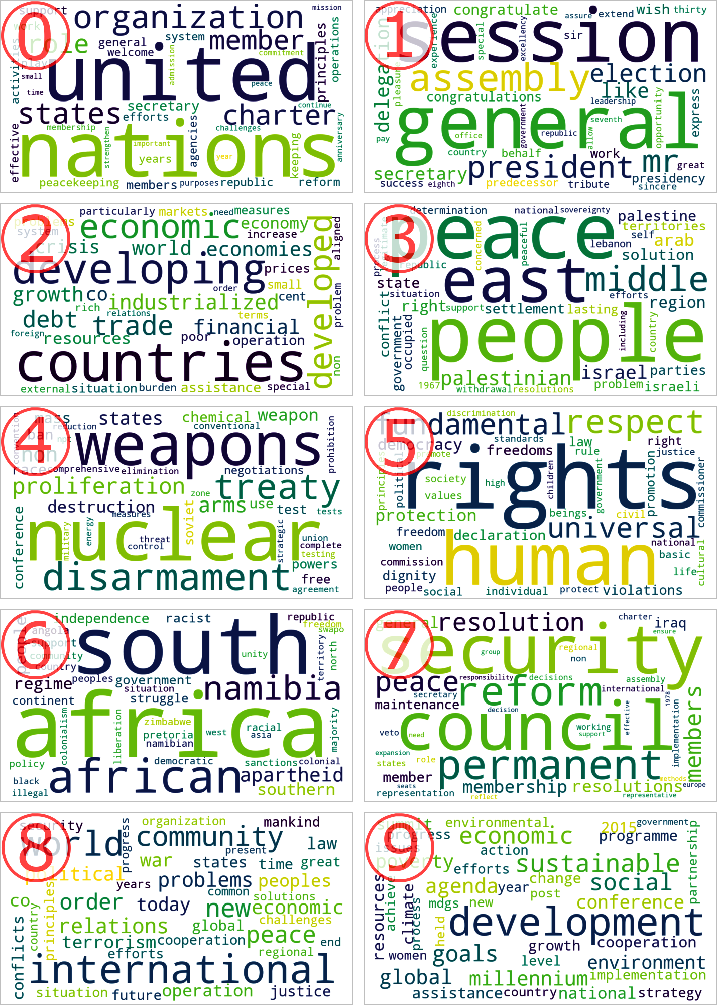
Figure 8-4. Word clouds representing the NMF topic model.
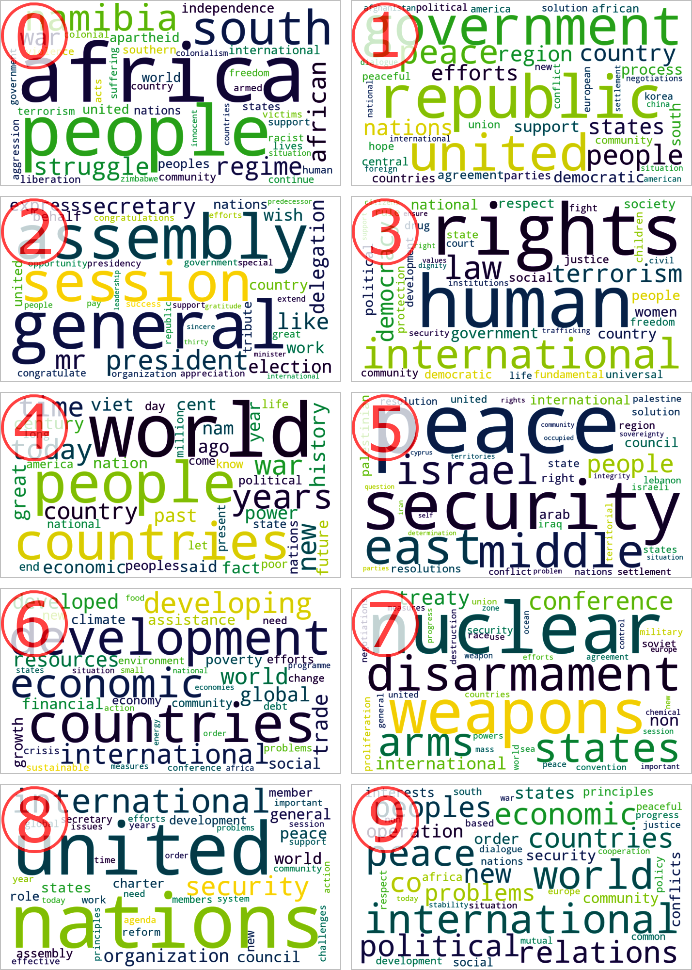
Figure 8-5. Word clouds representing the LDA topic model.
Blueprint: Calculating Topic Distribution of Documents and Time Evolution
As you can see in the analysis at the beginning of the chapter, the speech metadata changes over time. This leads to the interesting question of how the distribution of the topics changes over time. It turns out that this is easy to calculate and insightful.
Like the scikit-learn vectorizers, the topic models also have a transform method, which calculates the topic distribution of existing documents keeping the already fitted topic model. Let’s use this to first separate speeches before 1990 from those after 1990. For this, we create NumPy arrays for the documents before and after 1990:
importnumpyasnpbefore_1990=np.array(paragraph_df["year"]<1990)after_1990=~before_1990
Then we can calculate the respective W matrices:
W_para_matrix_early=nmf_para_model.transform(tfidf_para_vectors[before_1990])W_para_matrix_late=nmf_para_model.transform(tfidf_para_vectors[after_1990])(W_para_matrix_early.sum(axis=0)/W_para_matrix_early.sum()*100.0)(W_para_matrix_late.sum(axis=0)/W_para_matrix_late.sum()*100.0)
Out:
['9.34','10.43','12.18','12.18','7.82','6.05','12.10','5.85','17.36','6.69']['7.48','8.34','9.75','9.75','6.26','4.84','9.68','4.68','13.90','5.36']
The result is interesting, as some percentages have changed considerably; specifically, the size of the second-to-last topic is much smaller in the later years. We will now try to take a deeper look at the topics and their changes over time.
Let’s try to calculate the distribution for individual years and see whether we can find a visualization to uncover possible patterns:
year_data=[]years=np.unique(paragraph_years)foryearintqdm(years):W_year=nmf_para_model.transform(tfidf_para_vectors[paragraph_years\==year])year_data.append([year]+list(W_year.sum(axis=0)/W_year.sum()*100.0))
To make the plots more intuitive, we first create a list of topics with their two most important words:
topic_names=[]voc=tfidf_para_vectorizer.get_feature_names()fortopicinnmf_para_model.components_:important=topic.argsort()top_word=voc[important[-1]]+" "+voc[important[-2]]topic_names.append("Topic "+top_word)
We then combine the results in a DataFrame with the previous topics as column names, so we can easily visualize that as follows:
df_year=pd.DataFrame(year_data,columns=["year"]+topic_names).set_index("year")df_year.plot.area()
Out:
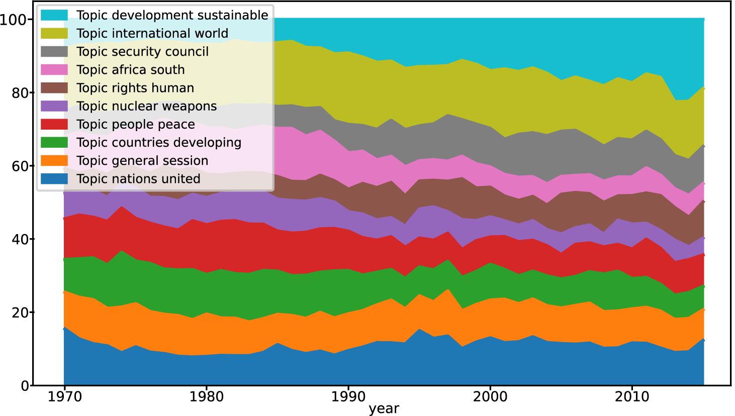
In the resulting graph you can see how the topic distribution changes over the year. We can recognize that the “sustainable development” topic is continuously increasing, while “south africa” has lost popularity after the apartheid regime ended.
Compared to showing the time development of single (guessed) words, topics seem to be a more natural entity as they arise from the text corpus itself. Note that this chart was generated with an unsupervised method exclusively, so there is no bias in it. Everything was already in the debates data; we have just uncovered it.
So far, we have used scikit-learn exclusively for topic modeling. In the Python ecosystem, there is a specialized library for topic models called Gensim, which we will now investigate.
Using Gensim for Topic Modeling
Apart from scikit-learn, Gensim is another popular tool for performing topic modeling in Python. Compared to scikit-learn, it offers more algorithms for calculating topic models and can also give estimates about the quality of the model.
Blueprint: Preparing Data for Gensim
Before we can start calculating the Gensim models, we have to prepare the data. Unfortunately, the API and the terminology are different from scikit-learn. In the first step, we have to prepare the vocabulary. Gensim has no integrated tokenizer and expects each line of a document corpus to be already tokenized:
# create tokenized documentsgensim_paragraphs=[[wforwinre.findall(r'\b\w\w+\b',paragraph.lower())ifwnotinstopwords]forparagraphinparagraph_df["text"]]
After tokenization, we can initialize the Gensim dictionary with these tokenized documents. Think of the dictionary as a mapping from words to columns (like the features we used in Chapter 2):
fromgensim.corporaimportDictionarydict_gensim_para=Dictionary(gensim_paragraphs)
Similar to the scikit-learn TfidfVectorizer, we can reduce the vocabulary by filtering out words that appear not often enough or too frequently. To keep the dimensions low, we choose a minimum of five documents in which words must appear, but not in more than 70% of the documents. As we saw in Chapter 2, these parameters can be optimized and require some experimentation.
In Gensim, this is implemented via a filter with the parameters no_below and no_above (in scikit-learn, the analog would be min_df and max_df):
dict_gensim_para.filter_extremes(no_below=5,no_above=0.7)
With the dictionary read, we can now use Gensim to calculate the bag-of-words matrix (which is called a corpus in Gensim, but we will stick with our current terminology):
bow_gensim_para=[dict_gensim_para.doc2bow(paragraph)\forparagraphingensim_paragraphs]
Finally, we can perform the TF-IDF transformation. The first line fits the bag-of-words model, while the second line transforms the weights:
fromgensim.modelsimportTfidfModeltfidf_gensim_para=TfidfModel(bow_gensim_para)vectors_gensim_para=tfidf_gensim_para[bow_gensim_para]
The vectors_gensim_para matrix is the one that we will use for all upcoming topic modeling tasks with Gensim.
Blueprint: Performing Nonnegative Matrix Factorization with Gensim
Let’s check first the results of NMF and see whether we can reproduce those of scikit-learn:
fromgensim.models.nmfimportNmfnmf_gensim_para=Nmf(vectors_gensim_para,num_topics=10,id2word=dict_gensim_para,kappa=0.1,eval_every=5)
The evaluation can take a while. Although Gensim offers a show_topics method for directly displaying the topics, we have a different implementation to make it look like the scikit-learn results so it’s easier to compare them:
display_topics_gensim(nmf_gensim_para)
Out:
| Topic 00 nations (0.03) united (0.02) human (0.02) rights (0.02) role (0.01) |
Topic 01 africa (0.02) south (0.02) people (0.02) government (0.01) republic (0.01) |
Topic 02 economic (0.01) development (0.01) countries (0.01) social (0.01) international (0.01) |
Topic 03 countries (0.02) developing (0.02) resources (0.01) sea (0.01) developed (0.01) |
Topic 04 israel (0.02) arab (0.02) palestinian (0.02) council (0.01) security (0.01) |
| Topic 05 organization (0.02) charter (0.02) principles (0.02) member (0.01) respect (0.01) |
Topic 06 problem (0.01) solution (0.01) east (0.01) situation (0.01) problems (0.01) |
Topic 07 nuclear (0.02) co (0.02) operation (0.02) disarmament (0.02) weapons (0.02) |
Topic 08 session (0.02) general (0.02) assembly (0.02) mr (0.02) president (0.02) |
Topic 09 world (0.02) peace (0.02) peoples (0.02) security (0.01) states (0.01) |
NMF is also a statistical method, so the results are not supposed to be identical to the ones that we calculated with scikit-learn, but they are similar enough. Gensim has code for calculating the coherence score for topic models, a quality indicator. Let’s try this:
fromgensim.models.coherencemodelimportCoherenceModelnmf_gensim_para_coherence=CoherenceModel(model=nmf_gensim_para,texts=gensim_paragraphs,dictionary=dict_gensim_para,coherence='c_v')nmf_gensim_para_coherence_score=nmf_gensim_para_coherence.get_coherence()(nmf_gensim_para_coherence_score)
Out:
0.6500661701098243
The score varies with the number of topics. If you want to find the optimal number of topics, a frequent approach is to run NMF for several different values, calculate the coherence score, and take the number of topics that maximizes the score.
Let’s try the same with LDA and compare the quality indicators.
Blueprint: Using LDA with Gensim
Running LDA with Gensim is as easy as using NMF if we have the data prepared. The LdaModel class has a lot of parameters for tuning the model; we use the recommended values here:
fromgensim.modelsimportLdaModellda_gensim_para=LdaModel(corpus=bow_gensim_para,id2word=dict_gensim_para,chunksize=2000,alpha='auto',eta='auto',iterations=400,num_topics=10,passes=20,eval_every=None,random_state=42)
We are interested in the word distribution of the topics:
display_topics_gensim(lda_gensim_para)
Out:
| Topic 00 climate (0.12) convention (0.03) pacific (0.02) environmental (0.02) sea (0.02) |
Topic 01 country (0.05) people (0.05) government (0.03) national (0.02) support (0.02) |
Topic 02 nations (0.10) united (0.10) human (0.04) security (0.03) rights (0.03) |
Topic 03 international (0.03) community (0.01) efforts (0.01) new (0.01) global (0.01) |
Topic 04 africa (0.06) african (0.06) continent (0.02) terrorist (0.02) crimes (0.02) |
| Topic 05 world (0.05) years (0.02) today (0.02) peace (0.01) time (0.01) |
Topic 06 peace (0.03) conflict (0.02) region (0.02) people (0.02) state (0.02) |
Topic 07 south (0.10) sudan (0.05) china (0.04) asia (0.04) somalia (0.04) |
Topic 08 general (0.10) assembly (0.09) session (0.05) president (0.04) secretary (0.04) |
Topic 09 development (0.07) countries (0.05) economic (0.03) sustainable (0.02) 2015 (0.02) |
The topics are not as easy to interpret as the ones generated by NMF. Checking the coherence score as shown earlier, we find a lower score of 0.45270703180962374. Gensim also allows us to calculate the perplexity score of an LDA model. Perplexity measures how well a probability model predicts a sample. When we execute lda_gensim_para.log_perplexity(vectors_gensim_para), we get a perplexity score of -9.70558947109483.
Blueprint: Calculating Coherence Scores
Gensim can also calculate topic coherence. The method itself is a four-stage process consisting of segmentation, probability estimation, a confirmation measure calculation, and aggregation. Fortunately, Gensim has a CoherenceModel class that encapsulates all these single tasks, and we can directly use it:
fromgensim.models.coherencemodelimportCoherenceModellda_gensim_para_coherence=CoherenceModel(model=lda_gensim_para,texts=gensim_paragraphs,dictionary=dict_gensim_para,coherence='c_v')lda_gensim_para_coherence_score=lda_gensim_para_coherence.get_coherence()(lda_gensim_para_coherence_score)
Out:
0.5444930496493174
Substituting nmf for lda, we can calculate the same score for our NMF model:
nmf_gensim_para_coherence=CoherenceModel(model=nmf_gensim_para,texts=gensim_paragraphs,dictionary=dict_gensim_para,coherence='c_v')nmf_gensim_para_coherence_score=nmf_gensim_para_coherence.get_coherence()(nmf_gensim_para_coherence_score)
Out:
0.6505110480127619
The score is quite a bit higher, which means that the NMF model is a better approximation to the real topics compared to LDA.
Calculating the coherence score of the individual topics for LDA is even easier, as it is directly supported by the LDA model. Let’s take a look at the average first:
top_topics=lda_gensim_para.top_topics(vectors_gensim_para,topn=5)avg_topic_coherence=sum([t[1]fortintop_topics])/len(top_topics)('Average topic coherence:%.4f.'%avg_topic_coherence)
Out:
Average topic coherence: -2.4709.
We are also interested in the coherence scores of the individual topics, which is contained in top_topics. However, the output is verbose (check it!), so we try to condense it a bit by just printing the coherence scores together with the most important words of the topics:
[(t[1]," ".join([w[1]forwint[0]]))fortintop_topics]
Out:
[(-1.5361194241843663,'general assembly session president secretary'),(-1.7014902754187737,'nations united human security rights'),(-1.8485895463251694,'country people government national support'),(-1.9729985026779555,'peace conflict region people state'),(-1.9743434414778658,'world years today peace time'),(-2.0202823396586433,'international community efforts new global'),(-2.7269347656599225,'development countries economic sustainable 2015'),(-2.9089975883502706,'climate convention pacific environmental sea'),(-3.8680684770508753,'africa african continent terrorist crimes'),(-4.1515707817343195,'south sudan china asia somalia')]
Coherence scores for topic models can easily be calculated using Gensim. The absolute values are difficult to interpret, but varying the methods (NMF versus LDA) or the number of topics can give you ideas about which way you want to proceed in your topic models. Coherence scores and coherence models are a big advantage of Gensim, as they are not (yet) included in scikit-learn.
As it’s difficult to estimate the “correct” number of topics, we are now taking a look at an approach that creates hierarchical models and does not need a fixed number of topics as a parameter.
Blueprint: Finding the Optimal Number of Topics
In the previous sections, we have always worked with 10 topics. So far we have not compared the quality of this topic model to different ones with a lower or higher number of topics. We want to find the optimal number of topics in a structured way without having to go into the interpretation of each constellation.
It turns out there is a way to achieve this. The “quality” of a topic model can be measured by the previously introduced coherence score. To find the best coherence score, we will now calculate it for a different number of topics with an LDA model. We will try to find the highest score, which should give us the optimal number of topics:
fromgensim.models.ldamulticoreimportLdaMulticorelda_para_model_n=[]fornintqdm(range(5,21)):lda_model=LdaMulticore(corpus=bow_gensim_para,id2word=dict_gensim_para,chunksize=2000,eta='auto',iterations=400,num_topics=n,passes=20,eval_every=None,random_state=42)lda_coherence=CoherenceModel(model=lda_model,texts=gensim_paragraphs,dictionary=dict_gensim_para,coherence='c_v')lda_para_model_n.append((n,lda_model,lda_coherence.get_coherence()))
Coherence Calculations Take Time
Calculating the LDA model (and the coherence) is computationally expensive, so in real life it would be better to optimize the algorithm to calculate only a minimal number of models and perplexities. Sometimes it might make sense if you calculate the coherence scores for only a few numbers of topics.
Now we can choose which number of topics produces a good coherence score. Note that typically the score grows with the number of topics. Taking too many topics makes interpretation difficult:
pd.DataFrame(lda_para_model_n,columns=["n","model",\"coherence"]).set_index("n")[["coherence"]].plot(figsize=(16,9))
Out:

Overall, the graph grows with the number of topics, which is almost always the case. However, we can see “spikes” at 13 and 17 topics, so these numbers look like good choices. We will visualize the results for 17 topics:
display_topics_gensim(lda_para_model_n[12][1])
Out:
| Topic 00 peace (0.02) international (0.02) cooperation (0.01) countries (0.01) region (0.01) |
Topic 01 general (0.05) assembly (0.04) session (0.03) president (0.03) mr (0.03) |
Topic 02 united (0.04) nations (0.04) states (0.03) european (0.02) union (0.02) |
Topic 03 nations (0.07) united (0.07) security (0.03) council (0.02) international (0.02) |
Topic 04 development (0.03) general (0.02) conference (0.02) assembly (0.02) sustainable (0.01) |
Topic 05 international (0.03) terrorism (0.03) states (0.01) iraq (0.01) acts (0.01) |
| Topic 06 peace (0.03) east (0.02) middle (0.02) israel (0.02) solution (0.01) |
Topic 07 africa (0.08) south (0.05) african (0.05) namibia (0.02) republic (0.01) |
Topic 08 states (0.04) small (0.04) island (0.03) sea (0.02) pacific (0.02) |
Topic 09 world (0.03) international (0.02) problems (0.01) war (0.01) peace (0.01) |
Topic 10 human (0.07) rights (0.06) law (0.02) respect (0.02) international (0.01) |
Topic 11 climate (0.03) change (0.03) global (0.02) environment (0.01) energy (0.01) |
| Topic 12 world (0.03) people (0.02) future (0.01) years (0.01) today (0.01) |
Topic 13 people (0.03) independence (0.02) peoples (0.02) struggle (0.01) countries (0.01) |
Topic 14 people (0.02) country (0.02) government (0.02) humanitarian (0.01) refugees (0.01) |
Topic 15 countries (0.05) development (0.03) economic (0.03) developing (0.02) trade (0.01) |
Topic 16 nuclear (0.06) weapons (0.04) disarmament (0.03) arms (0.03) treaty (0.02) |
Most of the topics are easy to interpret, but quite a few are difficult (like 0, 3, 8) as they contain many words with small, but not too different, sizes. Is the topic model with 17 topics therefore easier to explain? Not really. The coherence measure is higher, but that does not necessarily mean a more obvious interpretation. In other words, relying solely on coherence scores can be dangerous if the number of topics gets too large. Although in theory higher coherence should contribute to better interpretability, it is often a trade-off, and choosing smaller numbers of topics can make life easier. Taking a look back at the coherence graph, 10 seems to be a good value as it is a local maximum of the coherence score.
As it’s obviously difficult to find the “correct” number of topics, we will now take a look at an approach that creates hierarchical models and does not need a fixed number of topics as a parameter.
Blueprint: Creating a Hierarchical Dirichlet Process with Gensim
Take a step back and recall the visualization of the topics in “Blueprint: Using LDA with Gensim”. The sizes of the topics vary quite a bit, and some topics have a large overlap. It would be nice if the results gave us broader topics first and some subtopics below them. This is the exact idea of the hierarchical Dirichlet process (HDP). The hierarchical topic model should give us just a few broad topics that are well separated, then go into more detail by adding more words and getting more differentiated topic definitions.
HDP is still quite new and has not yet been extensively analyzed. Gensim is also often used in research and has an experimental implementation of HDP integrated. As we can directly use our already existing vectorization, it’s not complicated to try it. Note that we are again using the bag-of-words vectorization as the Dirichlet processes themselves handle frequent words correctly:
fromgensim.modelsimportHdpModelhdp_gensim_para=HdpModel(corpus=bow_gensim_para,id2word=dict_gensim_para)
HDP can estimate the number of topics and can show all that it identified:
hdp_gensim_para.print_topics(num_words=10)
Out:

The results are sometimes difficult to understand. It can be an option to first perform a “rough” topic modeling with only a few topics. If you find out that a topic is really big or suspect that it might have subtopics, you can create a subset of the original corpus where the only documents included are those that have a significant mixture of this topic. This needs some manual interaction but often yields much better results compared to HDP. At this stage of development, we would not recommend using HDP exclusively.
Topic models focus on uncovering the topic structure of a large corpus of documents. As all documents are modeled as a mixture of different topics, they are not well-suited for assigning documents to exactly one topic. This can be achieved using clustering.
Blueprint: Using Clustering to Uncover the Structure of Text Data
Apart from topic modeling, there is a multitude of other unsupervised methods. Not all are suitable for text data, but many clustering algorithms can be used. Compared to topic modeling, it is important for us to know that each document (or paragraph) gets assigned to exactly one cluster.
Clustering Works Well for Mono-Typical Texts
In our case, it is a reasonable assumption that each document belongs to exactly one cluster, as there are probably not too many different things contained in one paragraph. For larger text fragments, we would rather use topic modeling to take possible mixtures into account.
Most clustering methods need the number of clusters as a parameter, while there are a few (like mean-shift) that can guess the correct number of clusters. Most of the latter do not work well with sparse data and therefore are not suitable for text analytics. In our case, we decided to use k-means clustering, but birch or spectral clustering should work in a similar manner. There are a few nice explanations of how the k-means algorithm works.4
Clustering Is Much Slower Than Topic Modeling
For most algorithms, clustering takes considerable time, much more than even LDA. So, be prepared to wait for roughly one hour when executing the clustering in the next code fragment.
The scikit-learn API for clustering is similar to what we have seen with topic models:
fromsklearn.clusterimportKMeansk_means_text=KMeans(n_clusters=10,random_state=42)k_means_text.fit(tfidf_para_vectors)
KMeans(n_clusters=10,random_state=42)
But now it’s much easier to find out how many paragraphs belong to which cluster. Everything necessary is in the labels_ field of the k_means_para object. For each document, it contains the label that was assigned by the clustering algorithm:
np.unique(k_means_para.labels_,return_counts=True)
Out:
(array([0,1,2,3,4,5,6,7,8,9],dtype=int32),array([133370,41705,12396,9142,12674,21080,19727,10563,10437,11116]))
In many cases, you might already have found some conceptual problems here. If the data is too heterogeneous, most clusters tend to be small (containing a comparatively small vocabulary) and are accompanied by a large cluster that absorbs all the rest. Fortunately (and due to the short paragraphs), this is not the case here; cluster 0 is much bigger than the others, but it’s not orders of magnitude. Let’s visualize the distribution with the y-axis showing the size of the clusters (Figure 8-6):
sizes=[]foriinrange(10):sizes.append({"cluster":i,"size":np.sum(k_means_para.labels_==i)})pd.DataFrame(sizes).set_index("cluster").plot.bar(figsize=(16,9))
Visualizing the clusters works in a similar way to the topic models. However, we have to calculate the individual feature contributions manually. For this, we add up the TF-IDF vectors of all documents in the cluster and keep only the largest values.
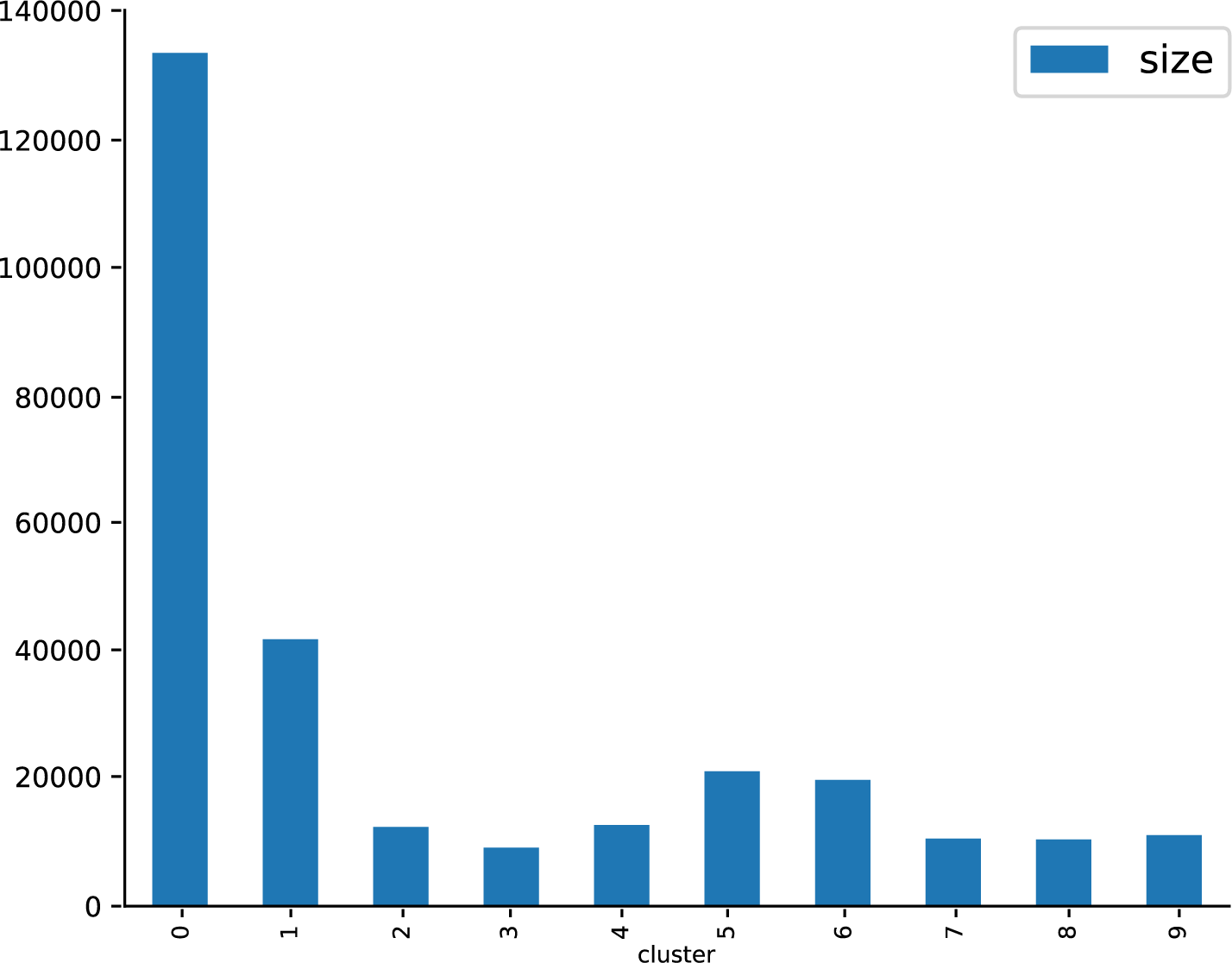
Figure 8-6. Visualization of the size of the clusters.
These are the weights for their corresponding words. In fact, that’s the only change compared to the previous code:
defwordcloud_clusters(model,vectors,features,no_top_words=40):forclusterinnp.unique(model.labels_):size={}words=vectors[model.labels_==cluster].sum(axis=0).A[0]largest=words.argsort()[::-1]# invert sort orderforiinrange(0,no_top_words):size[features[largest[i]]]=abs(words[largest[i]])wc=WordCloud(background_color="white",max_words=100,width=960,height=540)wc.generate_from_frequencies(size)plt.figure(figsize=(12,12))plt.imshow(wc,interpolation='bilinear')plt.axis("off")# if you don't want to save the topic model, comment the next lineplt.savefig(f'cluster{cluster}.png')wordcloud_clusters(k_means_para,tfidf_para_vectors,tfidf_para_vectorizer.get_feature_names())
Out:
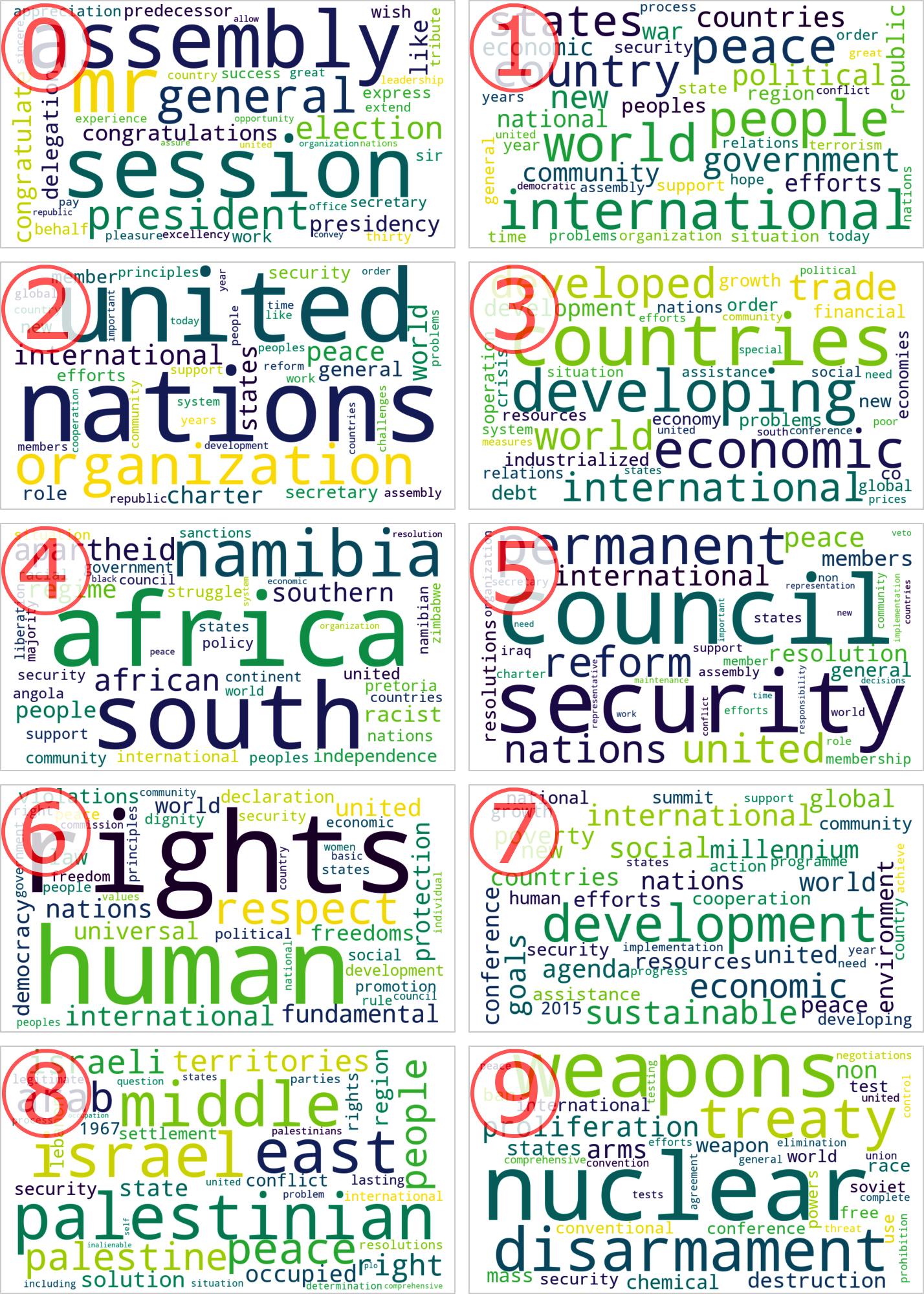
As you can see, the results are (fortunately) not too different from the various topic modeling approaches; you might recognize the topics of nuclear weapons, South Africa, general assembly, etc. Note, however, that the clusters are more pronounced. In other words, they have more specific words. Unfortunately, this is not true for the biggest cluster, 1, which has no clear direction but many words with similar, smaller sizes. This is a typical phenomenon of clustering algorithms compared to topic modeling.
Clustering calculations can take quite long, especially compared to NMF topic models. On the positive side, we are now free to choose documents in a certain cluster (opposed to a topic model, this is well-defined) and perform additional, more sophisticated operations, such as hierarchical clustering, etc.
The quality of the clustering can be calculated by using coherence or the Calinski-Harabasz score. These metrics are not optimized for sparse data and take a long time to calculate, and therefore we skip this here.
Further Ideas
In this chapter, we have shown different methods for performing topic modeling. However, we have only scratched the surface of the possibilities:
- It’s possible to add n-grams in the vectorization process. In scikit-learn this is straightforward by using the
ngram_rangeparameter. Gensim has a specialPhrasesclass for that. Due to the higher TF-IDF weights of n-grams, they can contribute considerably to the features of a topic and add a lot of context information. - As we have used years to have time-dependent topic models, you could also use countries or continents and find the topics that are most relevant in the speeches of their ambassadors.
- Calculate the coherence score for an LDA topic model using the whole speeches instead of the paragraphs and compare the scores.
Summary and Recommendation
In your daily work, it might turn out that unsupervised methods such as topic modeling or clustering are often used as first methods to understand the content of unknown text corpora. It is further useful to check whether the right features have been chosen or this can still be optimized.
One of the most important decisions is the entity on which you will be calculating the topics. As shown in our blueprint example, documents don’t always have to be the best choice, especially when they are quite long and consist of algorithmically determinable subentities.
Finding the correct number of topics is always a challenge. Normally, this must be solved iteratively by calculating the quality indicators. A frequently used, more pragmatic approach is to try with a reasonable number of topics and find out whether the results can be interpreted.
Using a (much) higher number of topics (like a few hundred), topic models are often used as techniques for the dimensionality reduction of text documents. With the resulting vectorizations, similarity scores can then be calculated in the latent space and frequently yield better results compared to the naive distance in TF-IDF space.
Conclusion
Topic models are a powerful technique and are not computationally expensive. Therefore, they can be used widely in text analytics. The first and foremost reason to use them is uncovering the latent structure of a document corpus.
Topic models are also useful for getting a summarization and an idea about the structure of large unknown texts. For this reason, they are often used routinely in the beginning of an analysis.
As there is a large number of different algorithms and implementations, it makes sense to experiment with the different methods and see which one yields the best results for a given text corpus. The linear-algebra-based methods are quite fast and make analyses possible by changing the number of topics combined with calculating the respective quality indicators.
Aggregating data in different ways before performing topic modeling can lead to interesting variations. As we have seen in the UN general debates dataset, paragraphs were more suited as the speakers talked about one topic after the other. If you have a corpus with texts from many authors, concatenating all texts per author will give you persona models for different types of authors.
1 Blei, David M., et al. “Latent Dirichlet Allocation.” Journal of Machine Learning Research 3 (4–5): 993–1022. doi:10.1162/jmlr.2003.3.4-5.993.
2 For a more detailed description, see the Wikipedia page.
3 pyLDAvis must be installed separately using pip install pyldavis or conda install pyldavis.
4 See, for example, Andrey A. Shabalin’s k-means clustering page or Naftali Harris’s “Visualizing K-Means Clustering”.