Chapter 13. Using Text Analytics in Production
We have introduced several blueprints so far and understood their application to multiple use cases. Any analysis or machine learning model is most valuable when it can be used easily by others. In this chapter, we will provide blueprints that will allow you to share the text classifier from one of our earlier chapters and also deploy to a cloud environment allowing anybody to make use of what we’ve built.
Consider that you used one of the blueprints in Chapter 10 in this book to analyze various car models using data from Reddit. If one of your colleagues was interested in doing the same analysis for the motorcycle industry, it should be simple to change the data source and reuse the code. In practice, this can prove much more difficult because your colleague will first have to set up an environment similar to the one you used by installing the same version of Python and all the required packages. It’s possible that they might be working on a different operating system where the installation steps are different. Or consider that the clients to whom you presented the analysis are extremely happy and come back three months later asking you to cover many more industries. Now you have to repeat the same analysis but ensure that the code and environment remain the same. The volume of data for this analysis could be much larger, and your system resources may not be sufficient enough, prompting a move to use cloud computing resources. You would have to go through the installation steps on a cloud provider, and this can quickly become time-consuming.
What You’ll Learn and What We’ll Build
Often what happens is that you are able to produce excellent results, but they remain unusable because other colleagues who want to use them are unable to rerun the code and reproduce the results. In this chapter, we will show you some techniques that can ensure that your analysis or algorithm can be easily repeated by anyone else, including yourself at a later stage. What if we are able to make it even easier for others to use the output of our analysis? This removes an additional barrier and increases the accessibility of our results. We will show you how you can deploy your machine learning model as a simple REST API that allows anyone to use the predictions from your model in their own work or applications. Finally, we will show you how to make use of cloud infrastructure for faster runtimes or to serve multiple applications and users. Since most production servers and services run Linux, this chapter includes a lot of executable commands and instructions that run best in a Linux shell or terminal. However, they should work just as well in Windows PowerShell.
Blueprint: Using Conda to Create Reproducible Python Environments
The blueprints introduced in this book use Python and the ecosystem of packages to accomplish several text analytics tasks. As with any programming language, Python has frequent updates and many supported versions. In addition, commonly used packages like Pandas, NumPy, and SciPy also have regular release cycles when they upgrade to a new version. While the maintainers try to ensure that newer versions are backward compatible, there is a risk that an analysis you completed last year will no longer be able to run with the latest version of Python. Your blueprint might have used a method that is deprecated in the latest version of a library, and this would make your analysis nonreproducible without knowing the version of the library used.
Let’s suppose that you share a blueprint with your colleague in the form of a Jupyter notebook or a Python module; one of the common errors they might face when trying to run is as shown here:
importspacy
Out:
---------------------------------------------------------------------------
ModuleNotFoundError                       Traceback (most recent call last)
<ipython-input-1-76a01d9c502b> in <module>
----> 1 import spacy
ModuleNotFoundError: No module named 'spacy'
In most cases, ModuleNotFoundError can be easily resolved by manually installing the required package using the command pip install <module_name>. But imagine having to do this for every nonstandard package! This command also installs the latest version, which might not be the one you originally used. As a result, the best way to ensure reproducibility is to have a standardized way of sharing the Python environment that was used to run the analysis. We make use of the conda package manager along with the Miniconda distribution of Python to solve this problem.
Note
There are several ways to solve the problem of creating and sharing Python environments, and conda is just one of them. pip is the standard Python package installer that is included with Python and is widely used to install Python packages. venv can be used to create virtual environments where each environment can have its own version of Python and set of installed packages. Conda combines the functionality of a package installer and environment manager and therefore is our preferred option. It’s important to distinguish conda from the Anaconda/Miniconda distributions. These distributions include Python and conda along with essential packages required for working with data. While conda can be installed directly with pip, the easiest way is to install Miniconda, which is a small bootstrap version that contains conda, Python, and some essential packages they depend on.
First, we must install the Miniconda distribution with the following steps. This will create a base installation containing just Python, conda, and some essential packages like pip, zlib, etc. We can now create separate environments for each project that contains only the packages we need and are isolated from other such environments. This is useful since any changes you make such as installing additional packages or upgrading to a different Python version does not impact any other project or application as they use their own environment. We can do so by using the following command:
conda create -n env_name [list_of_packages]
Executing the previous command will create a new Python environment with the default version that was available when Miniconda was installed the first time. Let’s create our environment called blueprints where we explicitly specify the version of Python and the list of additional packages that we would like to install as follows:
$ conda create -n blueprints numpy pandas scikit-learn notebook python=3.8
Collecting package metadata (current_repodata.json): - done
Solving environment: \ done
 Package Plan
  environment location: /home/user/miniconda3/envs/blueprints
  added / updated specs:
    - notebook
    - numpy
    - pandas
    - python=3.8
    - scikit-learn

The following packages will be downloaded:

    package                    |            build
    ---------------------------|-----------------
    blas-1.0                   |              mkl           6 KB
    intel-openmp-2020.1        |              217         780 KB
    joblib-0.16.0              |             py_0         210 KB
    libgfortran-ng-7.3.0       |       hdf63c60_0        1006 KB
    mkl-2020.1                 |              217       129.0 MB
    mkl-service-2.3.0          |   py37he904b0f_0         218 KB
    mkl_fft-1.1.0              |   py37h23d657b_0         143 KB
    mkl_random-1.1.1           |   py37h0573a6f_0         322 KB
    numpy-1.18.5               |   py37ha1c710e_0           5 KB
    numpy-base-1.18.5          |   py37hde5b4d6_0         4.1 MB
    pandas-1.0.5               |   py37h0573a6f_0         7.8 MB
    pytz-2020.1                |             py_0         184 KB
    scikit-learn-0.23.1        |   py37h423224d_0         5.0 MB
    scipy-1.5.0                |   py37h0b6359f_0        14.4 MB
    threadpoolctl-2.1.0        |     pyh5ca1d4c_0          17 KB
    ------------------------------------------------------------
                                           Total:       163.1 MB

The following NEW packages will be INSTALLED:

  _libgcc_mutex      pkgs/main/linux-64::_libgcc_mutex-0.1-main
  attrs              pkgs/main/noarch::attrs-19.3.0-py_0
  backcall           pkgs/main/noarch::backcall-0.2.0-py_0
  blas               pkgs/main/linux-64::blas-1.0-mkl
  bleach             pkgs/main/noarch::bleach-3.1.5-py_0
  ca-certificates    pkgs/main/linux-64::ca-certificates-2020.6.24-0

(Output truncated)
Once the command has been executed, you can activate it by executing conda activate <env_name>, and you will notice that the command prompt is prefixed with the name of the environment. You can further verify that the version of Python is the same as you specified:
$ conda activate blueprints
(blueprints) $ python --version
Python 3.8
You can see the list of all environments on your system by using the command conda env list, as shown next. The output will include the base environment, which is the default environment created with the installation of Miniconda. An asterisk against a particular environment indicates the currently active one, in our case the environment we just created. Please make sure that you continue to use this environment when you work on your blueprint:
(blueprints) $ conda env list
# conda environments:
#
base                     /home/user/miniconda3
blueprints            *  /home/user/miniconda3/envs/blueprints
conda ensures that each environment can have its own versions of the same package, but this could come at the cost of increased storage since the same version of each package will be used in more than one environment. This is mitigated to a certain extent with the use of hard links, but it may not work in cases where a package uses hard-coded paths. However, we recommend creating another environment when you switch projects. But it is a good practice to remove unused environments using the command conda remove --name <env_name> --all.
The advantage of this approach is that when you want to share the code with someone else, you can specify the environment in which it should run. You can export the environment as a YAML file using the command conda env export > environment.yml. Ensure that you are in the desired environment (by running conda activate <environment_name>) before running this command:
(blueprints) $ conda env export > environment.yml
(blueprints) $ cat environment.yml
name: blueprints
channels:
  - defaults
dependencies:
  - _libgcc_mutex=0.1=main
  - attrs=19.3.0=py_0
  - backcall=0.2.0=py_0
  - blas=1.0=mkl
  - bleach=3.1.5=py_0
  - ca-certificates=2020.6.24=0
  - certifi=2020.6.20=py37_0
  - decorator=4.4.2=py_0
  - defusedxml=0.6.0=py_0
  - entrypoints=0.3=py37_0
  - importlib-metadata=1.7.0=py37_0
  - importlib_metadata=1.7.0=0
  - intel-openmp=2020.1=217
  - ipykernel=5.3.0=py37h5ca1d4c_0
(output truncated)
As shown in the output, the environment.yml file creates a listing of all the packages and their dependencies used in the environment. This file can be used by anyone to re-create the same environment by running the command conda env create -f environment.yml. However, this method can have cross-platform limitations since the dependencies listed in the YAML file are specific to the platform. So if you were working on a Windows system and exported the YAML file, it may not necessarily work on a macOS system.
This is because some of the dependencies required by a Python package are platform-dependent. For instance, the Intel MKL optimizations are specific to a certain architecture and can be replaced with the OpenBLAS library. To provide a generic environment file, we can use the command conda env export --from-history > environment.yml, which generates a listing of only the packages that were explicitly requested by you. You can see the following output of running this command, which lists only the packages we installed when creating the environment. Contrast this with the previous environment file that also listed packages like attrs and backcall, which are part of the conda environment but not requested by us. When such a YAML file is used to create an environment on a new platform, the default packages and their platform-specific dependencies will be identified and installed automatically by conda. In addition, the packages that we explicitly specified and their dependencies will be installed:
(blueprints) $ conda env export --from-history > environment.yml
(blueprints) $ cat environment.yml
name: blueprints
channels:
  - defaults
dependencies:
  - scikit-learn
  - pandas
  - notebook
  - python=3.8
  - numpy
prefix: /home/user/miniconda3/envs/blueprints
The disadvantage of using the --from-history option is that the created environment is not a replica of the original environment since the base packages and dependencies are platform specific and hence different. If the platform where this environment is to be used is the same, then we do not recommend using this option.
Blueprint: Using Containers to Create Reproducible Environments
While a package manager like conda helps in installing multiple packages and managing dependencies, there are several platform-dependent binaries that can still hinder reproducibility. To make things simpler, we make use of a layer of abstraction called containers. The name is derived from the shipping industry, where standard-sized shipping containers are used to transport all kinds of goods by ships, trucks, and rail. Regardless of the type of items or the mode of transport, the shipping container ensures that anyone adhering to that standard can transport those items. In a similar fashion, we use a Docker container to standardize the environment we work in and guarantee that an identical environment is re-created every time regardless of where it runs or who runs it. Docker is one of the most popular tools that enables this functionality, and we will make use of it in this blueprint. Figure 13-1 shows a high-level overview of how Docker works.

Figure 13-1. Workflow of Docker.
We need to start by installing Docker from the download link. Once it has been set up, please run sudo docker run hello-world from the command line to test that everything has been set up correctly, and you should see the output as shown. Please note that the Docker daemon binds to a Unix socket that is owned by the root user, hence the need to run all commands with sudo. If you are unable to provide root access, there is an experimental version of Docker that you can also try:
$ sudo docker run hello-world

Hello from Docker!
This message shows that your installation appears to be working correctly.

To generate this message, Docker took the following steps:
 1. The Docker client contacted the Docker daemon.
 2. The Docker daemon pulled the "hello-world" image from the Docker Hub.
    (amd64)
 3. The Docker daemon created a new container from that image which runs the
    executable that produces the output you are currently reading.
 4. The Docker daemon streamed that output to the Docker client, which sent it
    to your terminal.

To try something more ambitious, you can run an Ubuntu container with:
 $ docker run -it ubuntu bash

Share images, automate workflows, and more with a free Docker ID:
 https://hub.docker.com/

For more examples and ideas, visit:
 https://docs.docker.com/get-started/
We can draw an analogy between building a Docker container and purchasing a car. We start by choosing from one of the preconfigured options. These configurations already have some components selected, such as the type of engine (displacement, fuel-type), safety features, level of equipment, etc. We can customize many of these components, for example, upgrade to a more fuel-efficient engine or add additional components like a navigation system or heated seats. At the end, we decide on our preferred configuration and order the car. In a similar way, we specify the configuration of the environment we want to create in the Dockerfile. These are described in the form of a set of instructions, executed in a sequential manner resulting in the creation of a Docker image. A Docker image is like the preferred car configuration that can be created based on our Dockerfile. All Docker images are extensible, so instead of defining all steps, we could extend an existing Docker image and customize it by adding specific steps that we would like. The final step of running a Docker image results in the creation of a Docker container, which is like the car with your preferred configuration delivered to you. In this case, it is a full-fledged environment including an operating system and additional utilities and packages as specified in the Dockerfile. It runs on the hardware and uses the interfaces provided by the host system but is completely isolated from it. In effect, it is a minimal version of a server running the way you designed it. Each Docker container instantiated from the same image will be the same regardless of which host system it is running on. This is powerful as it allows you to encapsulate your analysis and environment and run it on your laptop, in the cloud, or on your organization’s server and expect the same behavior.
We are going to create a Docker image with the same Python environment as used in our analysis so that anyone else can reproduce our analysis by pulling the image and instantiating it as a container. While we can start by specifying our Docker image from scratch, it would be preferable to start with an existing image and customize certain parts of it to create our version. Such an image is referred to as a parent image. A good place to search for parent images is the Docker Hub registry, which is a public repository containing prebuilt Docker images. You will find officially supported images like the Jupyter Data Science notebook as well as user-created images like the one we have created for Chapter 9 that can be accessed here. Every image in the Docker repository can also be used as is to run containers. You can search for images using the sudo docker search command and add arguments to format results, as shown here where we search for available Miniconda images:
$ sudo docker search miniconda
NAME                                        STARS
continuumio/miniconda3                      218
continuumio/miniconda                       77
conda/miniconda3                            35
conda/miniconda3-centos7                    7
yamitzky/miniconda-neologd                  3
conda/miniconda2                            2
atavares/miniconda-rocker-geospatial        2
We see that there is an image for Miniconda3 that would be a good starting point for our own Dockerfile. Note that all Dockerfiles have to start with the FROM keyword specifying which image they are deriving from. If you are specifying a Dockerfile from the start, then you would use the FROM scratch keyword. The details of the Miniconda image and the Dockerfile show how this image derives from a Debian parent image and only adds additional steps to install and set up the conda package manager. When using a parent Docker image, it’s important to check that it’s from a trusted source. Docker Hub provides additional criteria like “Official Images” that can be helpful in identifying an official source.
Let’s walk through the steps defined in our Dockerfile. We start with the Miniconda3 image and then add a step to create our custom environment. We use the ARG instruction to specify the argument for the name of our conda environment (blueprints). We then use ADD to copy the environment.yml file from the build context to the image. Finally, we create the conda environment by providing the conda create command as an argument to RUN:
FROM continuumio/miniconda3

# Add environment.yml to the build context and create the environment
ARG conda_env=blueprints
ADD environment.yml /tmp/environment.yml
RUN conda env create -f /tmp/environment.yml
In the next set of steps, we want to ensure that the environment is activated in the container. Therefore, we add it to the end of the .bashrc script, which will always run when the container starts. We also update the PATH environment variable using the ENV instruction to ensure that the conda environment is the version of Python used everywhere within the container:
# Activating the environment and starting the jupyter notebook
RUN echo "source activate ${conda_env}" > ~/.bashrc
ENV PATH /opt/conda/envs/${conda_env}/bin:$PATH
In the final step, we want to automatically start a Jupyter notebook that will allow the users of this Docker container to run the analysis in an interactive fashion. We use the ENTRYPOINT instruction, which is used to configure a container that will run as an executable. There can be only one such instruction in a Dockerfile (if there are multiple, only the last one will be valid), and it will be the last command to run when a container comes up and is typically used to start a server like the Jupyter notebook that we want to run. We specify additional arguments to run the server on the IP address of the container itself (0.0.0.0), on a particular port (8888), as the root user (--allow-root), and not open a browser by default (--no-browser). When the container starts, we don’t want it to open the Jupyter server in its browser. Instead, we will attach the host machine to this container using the specified port and access it via the browser there:
# Start jupyter server on container
EXPOSE 8888
ENTRYPOINT ["jupyter","notebook","--ip=0.0.0.0", \
      "--port=8888","--allow-root","--no-browser"]
We use the docker build command to create the image from our Dockerfile. We specify the name of our image with the -t parameter and add a username followed by the name of the image. This is useful in identifying our image when we want to refer to it later. It is not mandatory to specify a username, but we will see later why this is useful. The Dockerfile to be used while building the image is specified with the -f parameter. If nothing is specified, then Docker will pick the file named Dockerfile in the directory specified by the argument PATH. The PATH argument also specifies where to find the files for the “context” of the build on the Docker daemon. All the files in this directory are packaged with tar and sent to the daemon during the build process. This must include all the files and artifacts that have to be added to the image, e.g., the environment.yml file, which will be copied to the image to create the conda environment.
docker build -t username/docker_project -f Dockerfile [PATH]
On executing this command, the Docker daemon starts creating an image by running the steps specified in the Dockerfile. Typically, you would execute the command in the same directory that already contains all the files and the Dockerfile as well. We specify the PATH argument using . referring to the current directory:
$ sudo docker build -t textblueprints/ch13:v1 .
Sending build context to Docker daemon  5.363MB
Step 1/8 : FROM continuumio/miniconda3
 ---> b4adc22212f1
Step 2/8 : ARG conda_env=blueprints
 ---> 959ed0c16483
Step 3/8 : ADD environment.yml /tmp/environment.yml
 ---> 60e039e09fa7
Step 4/8 : RUN conda env create -f /tmp/environment.yml
 ---> Running in 85d2f149820b
Collecting package metadata (repodata.json): ...working... done
Solving environment: ...working... done

Downloading and Extracting Packages

(output truncated)

Removing intermediate container 85d2f149820b
Step 5/8 : RUN echo "source activate ${conda_env}" > ~/.bashrc
 ---> e0ed2b448211
Step 6/8 : ENV PATH /opt/conda/envs/${conda_env}/bin:$PATH
 ---> 7068395ce2cf
Step 7/8 : EXPOSE 8888
 ---> Running in f78ac4aa0569
Removing intermediate container f78ac4aa0569
 ---> 06cfff710f8e
Step 8/8 : ENTRYPOINT ["jupyter","notebook","--ip=0.0.0.0",
                       "--port=8888","--allow-root","--no-browser"]
 ---> Running in 87852de682f4
Removing intermediate container 87852de682f4
 ---> 2b45bb18c071
Successfully built 2b45bb18c071
Successfully tagged textblueprints/ch13:v1
After the build completes, you can check whether the image was created successfully by running the command sudo docker images. You will notice that continuumio/miniconda3 image has been downloaded, and in addition, the image specified with your username and docker_project has also been created. Building a Docker will take longer the first time since the parent images have to be downloaded, but subsequent changes and rebuilds will be much faster:
$ sudo docker images
REPOSITORY                          TAG                 IMAGE ID
textblueprints/ch13                 v1                  83a05579afe6
jupyter/minimal-notebook            latest              d94723ae86d1
continuumio/miniconda3              latest              b4adc22212f1
hello-world                         latest              bf756fb1ae65
We can create a running instance of this environment, also called container, by running:
docker run -p host_port:container_port username/docker_project:tag_name
The -p argument allows port forwarding, essentially sending any requests received on the host_port to the container_port. By default, the Jupyter server can only access the files and directories within the container. However, we would like to access the Jupyter notebooks and code files present in a local directory from the Jupyter server running inside the container. We can attach a local directory to the container as a volume by using -v host_volume:container_volume, which will create a new directory within the container pointing to a local directory. This ensures that any changes made to the Jupyter notebooks are not lost when the container shuts down. This is the recommended approach to work with files locally but using a Docker container for the reproducible environment. Let’s start our Docker container by running the following command:
sudo docker run -p 5000:8888 -v \
/home/user/text-blueprints/ch13/:/work textblueprints/ch13:v1
Out:
[NotebookApp] Writing notebook server cookie secret to
/root/.local/share/jupyter/runtime/notebook_cookie_secret
[NotebookApp] Serving notebooks from local directory: /
[NotebookApp] The Jupyter Notebook is running at:
[NotebookApp] http://aaef990b90a3:8888/?token=xxxxxx
[NotebookApp]  or http://127.0.0.1:8888/?token=xxxxxx
[NotebookApp] Use Control-C to stop this server and shut down all kernels
(twice to skip confirmation).
[NotebookApp]

    To access the notebook, open this file in a browser:
        file:///root/.local/share/jupyter/runtime/nbserver-1-open.html
    Or copy and paste one of these URLs:
        http://aaef990b90a3:8888/?token=xxxxxx
     or http://127.0.0.1:8888/?token=xxxxxx
The logs you see now are actually the logs of the Jupyter server starting in port 8888 within the container. Since we have mapped the host port 5000, you can copy the URL and only replace the port number to 5000 to access the Jupyter server. You will also find here a directory called work, which should contain all the files from the local directory that was mapped. You can also check the status of all running containers by running the command sudo docker container ps. We can also specify the name for each running container by using the --name argument, and if this is not used, the Docker daemon will assign a randomly created one, as you see here:
$ sudo docker container ls
CONTAINER ID        IMAGE                    STATUS              NAMES
862e5b0570fe        textblueprints/ch13:v1   Up About a minute   musing_chaum
If you quit the terminal window where you ran this command, then the container will also be shut down. To run it in a detached mode, just add the -d option to the run command. When the container starts, it will print the container ID of the started container, and you can monitor the logs using sudo docker logs <container-id>. We have reproduced the complete environment used to run our analysis in this Docker container, and in the next blueprint, let’s see the best techniques to share it.
The easiest way to share this image with anyone is by pushing this to the Docker Hub registry. You can sign up for a free account. Docker Hub is a public repository for Docker images, and each image is uniquely identified by the username, the name of the image, and a tag. For example, the miniconda3 package that we used as our parent image is identified as continuumio/miniconda3:latest, and any images that you share will be identified with your username. Therefore, when we built our image earlier, the username we specified must have been the same as the one used to log in to Docker Hub. Once you have created your credentials, you can click Create a Repository and choose a name and provide a description for your repository. In our case we created a repository called "ch13" that will contain a Docker image for this chapter. Once done, you can log in using the command sudo docker login and enter your username and password. For added security, please follow the instructions to securely store your password.
Note
By default, during the build process of a Docker image, all of the directories and files present in the PATH argument are part of the build context. In a previous command, we indicated the path to be the current directory using the . symbol. This is not necessary since we need to include only the selected list of files that are needed for the build and later the container. For instance, we need environment.yml but not the Jupyter notebook (.ipynb) file. It’s important to specify the list of excluded files in the .dockerignore file to ensure that unwanted files do not automatically get added to the container. Our .dockerignore file is as shown here:
  .git
  .cache
  figures
  **/*.html
  **/*.ipynb
  **/*.css
Another thing to ensure is that the host_port (specified as 5000 in the blueprint) is open and not used by any other application on your system. Ideally, you must use a port number between 1024–49151 as these are user ports, but you can also check this easily by running the command sudo ss -tulw, which will provide the list of used ports.
The next step is to tag the image that you would like to share with a tag_name to identify what it contains. In our case, we tag the image with v1 to signify that it is the first version for this chapter. We run the command sudo docker tag 2b45bb18c071 textblueprints/ch13:v1, where 2b45bb18c071 is the image ID. We can push our file now with the command sudo docker push textblueprints/ch13. Now anyone who wants to run your project can simply run the command docker pull your_username/docker_project:tag_name to create the same environment as you, irrespective of the system they might be personally working on. As an example, you can start working on blueprints in Chapter 9 by simply running the command docker pull textblueprints/ch09:v1. You can then attach the volume of the directory containing the cloned repository. Docker Hub is a popular public registry and configured as default with Docker, but each cloud provider also has their own version, and many organizations set up private registries for use within their internal applications and teams.
When working with conda environments with multiple scientific computing packages, Docker images can get large and therefore create a strain on bandwidth while pushing to Docker Hub. A much more efficient way is to include the Dockerfile in the base path of your repository. For example, the GitHub repo containing the code for this chapter contains a Dockerfile, which can be used to create the exact environment required to run the code. This blueprint easily allows you to move an analysis from your local system to a cloud machine with additional resources by re-creating the same working environment. This is especially useful when the size of the data increases or an analysis takes too long to finish.
Blueprint: Creating a REST API for Your Text Analytics Model
Let’s say you used the blueprint provided in Chapter 11 to analyze the sentiment of customer support tickets in your organization. Your company is running a campaign to improve customer satisfaction where they would like to provide vouchers to unhappy customers. A colleague from the tech team reaches out to you for help with automating this campaign. While they can pull the Docker container and reproduce your analysis, they would prefer a simpler method where they provide the text of the support ticket and get a response of whether this is an unhappy customer. By encapsulating our analysis in a REST API, we can create a simple method that is accessible to anyone without them having to rerun the blueprint. They don’t even necessarily need to know Python since a REST API can be called from any language. In Chapter 2, we made use of REST APIs provided by popular websites to extract data, whereas in this blueprint we are going to create our own.
We will make use of the following three components to host our REST API:
- FastAPI: A fast web framework for building APIs
- Gunicorn: A Web Service Gateway Interface server that handles all the incoming requests
- Docker: Extending the Docker container that we used in the previous blueprint
Let’s create a new folder called app where we will place all the code that we require in order to serve sentiment predictions. It will follow the directory structure and contain files as shown next. main.py is where we will create the FastAPI app and the sentiment prediction method, and preprocessing.py is where our helper functions are included. The models directory contains the trained models we need to use to calculate our predictions, in our case the sentiment_vectorizer and sentiment_classification. Finally, we have the Dockerfile, environment.yml, and start_script.sh, which will be used to deploy our REST API:
├── app
│   ├── main.py
│   ├── Dockerfile
│   ├── environment.yml
│   ├── models
│   │   ├── sentiment_classification.pickle
│   │   └── sentiment_vectorizer.pickle
│   ├── preprocessing.py
│   └── start_script.sh
FastAPI is a fast Python framework used to build APIs. It is capable of redirecting requests from a web server to specific functions defined in Python. It also takes care of validating the incoming requests against specified schema and is useful for creating a simple REST API. We will encapsulate the predict function of the model we trained in Chapter 11 in this API. Let’s walk through the code in the file main.py step-by-step and explain how it works. You can install FastAPI by running pip install fastapi and Gunicorn by running pip install gunicorn.
Once FastAPI is installed, we can create an app using the following code:
fromfastapiimportFastAPIapp=FastAPI()
The FastAPI library runs this app using the included web server and can route requests received at an endpoint to a method in the Python file. This is specified by adding the @app.post attribute at the start of the function definition. We specify the endpoint to be api/v1/sentiment, the first version of our Sentiment API, which accepts HTTP POST requests. An API can evolve over time with changes to functionality, and it’s useful to separate them into different versions to ensure that users of the older version are not affected:
classSentiment(Enum):POSITIVE=1NEGATIVE=0@app.post("/api/v1/sentiment",response_model=Review)defpredict(review:Review,model=Depends(load_model())):text_clean=preprocessing.clean(review.text)text_tfidf=vectorizer.transform([text_clean])sentiment=prediction_model.predict(text_tfidf)review.sentiment=Sentiment(sentiment.item()).namereturnreview
The predict method retrieves the text field from the input and performs the preprocessing and vectorization steps. It uses the model we trained earlier to predict the sentiment of the product review. The returned sentiment is specified as an Enum class to restrict the possible return values for the API. The input parameter review is defined as an instance of the class Review. The class is as specified next and contains the text of the review, a mandatory field along with reviewerID, productID, and sentiment. FastAPI uses “type hints” to guess the type of the field (str) and perform the necessary validation. As we will see, FastAPI automatically generates a web documentation for our API following the OpenAPI specification from which the API can be tested directly. We add the schema_extra as an example to act as a guide to developers who want to use the API:
classReview(BaseModel):text:strreviewerID:Optional[str]=Noneasin:Optional[str]=Nonesentiment:Optional[str]=NoneclassConfig:schema_extra={"example":{"text":"This was a great purchase, saved me much time!","reviewerID":"A1VU337W6PKAR3","productID":"B00K0TIC56"}}
You would have noticed the use of the Depends keyword in the function definition. This allows us to load dependencies or other resources that are required before the function is called. This is treated as another Python function and is defined here:
defload_model():try:('Calling Depends Function')globalprediction_model,vectorizerprediction_model=pickle.load(open('models/sentiment_classification.pickle','rb'))vectorizer=pickle.load(open('models/tfidf_vectorizer.pickle','rb'))('Models have been loaded')exceptExceptionase:raiseValueError('No model here')
Note
Pickle is a Python serialization framework that is one of the common ways in which models can be saved/exported. Other standardized formats include joblib and ONNX. Some deep learning frameworks use their own export formats. For example, TensorFlow uses SavedModel, while PyTorch uses pickle but implements its own save() function. It’s important that you adapt the load and predict functions based on the type of model save/export you have used.
During development, FastAPI can be run with any web server (like uvicorn), but it is recommended to use a full-fledged Web Service Gateway Interface (WSGI) server, which is production ready and supports multiple worker threads. We choose to use Gunicorn as our WSGI server as it provides us with an HTTP server that can receive requests and redirect to the FastAPI app.
Once installed, it can be run by entering:
gunicorn -w 3 -b :5000 -t 5 -k uvicorn.workers.UvicornWorker main:app
The -w argument is used to specify the number of worker processes to run, three workers in this case. The -b parameter specifies the port that WSGI server listens on, and the -t indicates a timeout value of five seconds after which the server will kill and restart the app in case it’s not responsive. The -k argument specifies the instance of worker class (uvicorn) that must be called to run the app, which is specified by referring to the Python module (main) and the name (app).
Before deploying our API, we have to revisit the environment.yml file. In the first blueprint, we described ways to generate and share the environment.yml file to ensure that your analysis is reproducible. However, it is not recommended to follow this method when deploying code to production. While the exported environment.yml file is a starting point, we must inspect it manually and ensure that it does not contain unused packages. It’s also important to specify the exact version number of a package to ensure that package updates do not interfere with your production deployment. We use a Python code analysis tool called Vulture that identifies unused packages as well as other dead code fragments. Let’s run this analysis for the app folder:
vultureapp/
Out:
app/main.py:11: unused variable 'POSITIVE' (60% confidence)
app/main.py:12: unused variable 'NEGATIVE' (60% confidence)
app/main.py:16: unused variable 'reviewerID' (60% confidence)
app/main.py:17: unused variable 'asin' (60% confidence)
app/main.py:20: unused class 'Config' (60% confidence)
app/main.py:21: unused variable 'schema_extra' (60% confidence)
app/main.py:40: unused variable 'model' (100% confidence)
app/main.py:44: unused attribute 'sentiment' (60% confidence)
app/preprocessing.py:30: unused import 'spacy' (90% confidence)
app/preprocessing.py:34: unused function 'display_nlp' (60% confidence)
Along with the list of potential issues, Vulture also provides a confidence score. Please use the identified issues as pointers to check the use of these imports. In the previous example, we know that the class variables we have defined are used to validate the input to the API and are definitely used. We can see that even though spacy and display_nlp are part of the preprocessing module, they are not used in our app. We can choose to remove them and the corresponding dependencies from the YAML file.
You can also determine the version of each package used in the conda environment by running the conda list command and then use this information to create the final cleaned-up environment YAML file, as shown here:
name:sentiment-appchannels:-conda-forgedependencies:-python==3.8-fastapi==0.59.0-pandas==1.0.5-scikit-learn==0.23.2-gunicorn==20.0.4-uvicorn==0.11.3
As the final step, we can Dockerize the API so that it’s easier to run the entire app in its own container, which is especially beneficial when we want to host it on a cloud provider, as we will see in the next blueprint. We make two changes in the Dockerfile from the previous blueprint as follows:
# Copy files required for deploying service to app folder in container
COPY . /app
WORKDIR /app
The previous instruction is used to COPY all of the contents of the current app folder to the Docker image, which contains all of the files needed to deploy and run the REST API. The current directory in the container is then changed to the app folder by using the WORKDIR instruction:
# Start WSGI server on container
EXPOSE 5000
RUN ["chmod", "+x", "start_script.sh"]
ENTRYPOINT [ "/bin/bash", "-c" ]
CMD ["./start_script.sh"]
We then provide the steps to run the WSGI server by first exposing port 5000 on the container. Next, we enable permissions on the start_script so that the Docker daemon can execute it at container startup. We use a combination of ENTRYPOINT (used to start the bash shell in which the script is to be run) and CMD (used to specify the actual script as an argument to the bash shell), which activates the conda environment and starts the Gunicorn server. Since we are running the server within a Docker container, we make a small change to specify the access-logfile to be written to STDOUT (-) to ensure we can still view them:
#!/bin/bashsourceactivatemy_env_nameGUNICORN_CMD_ARGS="--access-logfile -"gunicorn-w3-b:5000-t5\-kuvicorn.workers.UvicornWorkermain:app-
We build the Docker image and run it following the same steps as in the previous blueprint. This will result in a running Docker container where the Gunicorn WSGI server is running the FastAPI app. We have to make sure that we forward a port from the host system where the container is running:
$ sudo docker run -p 5000:5000 textblueprints/sentiment-app:v1
    [INFO] Starting gunicorn 20.0.4
    [INFO] Listening at: http://0.0.0.0:5000 (11)
    [INFO] Using worker: sync
    [INFO] Booting worker with pid: 14
We can make a call to the container running the API from a different program. In a separate terminal window or IDE, create a test method that calls the API and passes in a sample review to check the response. We make a call to port 5000 with the local IP, which is forwarded to port 5000 of the container from which we receive the response, as shown here:
importrequestsimportjsonurl='http://0.0.0.0:5000/api/v1/sentiment'data={'text':'I could not ask for a better system for my small greenhouse,\easy to set up and nozzles do very well','reviewerID':'A1VU337W6PKAR3','productID':'B00K0TIC56'}input_data=json.dumps(data)headers={'content-type':'application/json','Accept-Charset':'UTF-8'}r=requests.post(url,data=input_data,headers=headers)(r.text)
Out:
{
  "prediction": "POSITIVE"
}
We can see that our API has generated the expected response. Let’s also check the documentation of this API, which we can find at http://localhost:5000/docs. It should generate a page as shown in Figure 13-2, and clicking the link for our /api/v1/sentiment method will provide additional details on how the method is to be called and also has the option to try it out. This allows others to provide different text inputs and view the results generated by the API without writing any code.
Docker containers are always started in unprivileged mode, meaning that even if there is a terminal error, it would only be restricted to the container without any impact to the host system. As a result, we can run the server as a root user safely within the container without worrying about an impact on the host system.
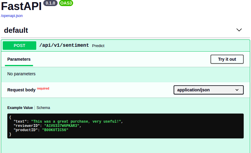
Figure 13-2. API specification and testing provided by FastAPI.
You can run a combination of the sudo docker tag and sudo docker push commands discussed earlier to share the REST API. Your colleague could easily pull this Docker image to run the API and use it to identify unhappy customers by providing their support tickets. In the next blueprint, we will run the Docker image on a cloud provider and make it available on the internet.
Blueprint: Deploying and Scaling Your API Using a Cloud Provider
Deploying machine learning models and monitoring their performance is a complex task and includes multiple tooling options. This is an area of constant innovation that is continuously looking to make it easier for data scientists and developers. There are several cloud providers and multiple ways to deploy and host your API using one of them. This blueprint introduces a simple way to deploy the Docker container we created in the previous blueprint using Kubernetes. Kubernetes is an open source technology that provides functionality to deploy and manage Docker containers to any underlying physical or virtual infrastructure. In this blueprint, we will be using Google Cloud Platform (GCP), but most major providers have support for Kubernetes. We can deploy the Docker container directly to a cloud service and make the REST API available to anyone. However, we choose to deploy this within a Kubernetes cluster since it gives us the flexibility to scale up and down the deployment easily.
You can sign up for a free account with GCP. By signing up with a cloud provider, you are renting computing resources from a third-party provider and will be asked to provide your billing details. During this blueprint, we will stay within the free-tier limit, but it’s important to keep a close track of your usage to ensure that you are not charged for some cloud resources that you forgot to shut down! Once you’ve completed the sign-up process, you can check this by visiting the Billing section from the GCP console. Before using this blueprint, please ensure that you have a Docker image containing the REST API pushed and available in Docker Hub or any other container registry.
Let’s start by understanding how we are going to deploy the REST API, which is illustrated in Figure 13-3. We will create a scalable compute cluster using GCP. This is nothing but a collection of individual servers that are called nodes. The compute cluster shown has three such nodes but can be scaled when needed. We will use Kubernetes to deploy the REST API to each node of the cluster. Assuming we start with three nodes, this will create three replicas of the Docker container, each running on one node. These containers are still not exposed to the internet, and we make use of Kubernetes to run a load balancer service, which provides a gateway to the internet and also redirects requests to each container depending on its utilization. In addition to simplifying our deployment process, the use of Kubernetes ensures that node failures and traffic spikes can be handled by automatically creating additional instances.

Figure 13-3. Kubernetes architecture diagram.
Let’s create a project in GCP that we will use for our deployment. Visit Google Cloud, choose the Create Project option on the top right, and create a project with your chosen name (we choose sentiment-rest-api). Once the project has been created, click the navigation menu on the top left and navigate to the service called Kubernetes Engine, as shown in Figure 13-4. You have to click the Enable Billing link and select the payment account that you set up when you signed up. You can also click the Billing tab directly and set it up for your project as well. Assuming you are using the free trial to run this blueprint, you will not be charged. It will take a few minutes before it gets enabled for our project. Once this is complete, we are ready to proceed with our deployment.
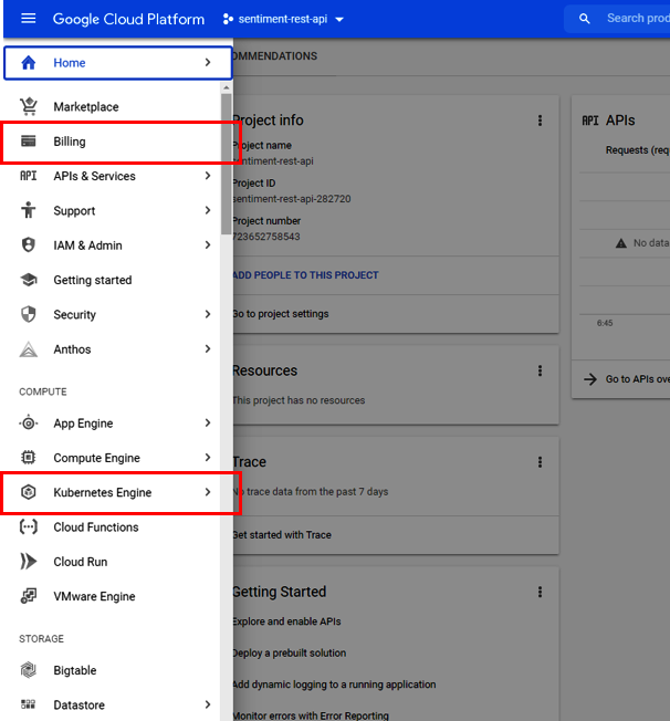
Figure 13-4. Enable Billing in the Kubernetes Engine option in the GCP console.
We can continue to work with Google Cloud Platform using the web console or the command-line tool. While the functionality offered remains the same, we choose to describe the steps in the blueprint with the help of the command-line interface in the interest of brevity and to enable you to copy the commands. Please install the Google Cloud SDK by following the instructions and then use the Kubernetes command-line tool by running:
gcloud components install kubectl
In a new terminal window, we first authenticate our user account by running gcloud auth login. This will open the browser and redirect you to the Google authentication page. Once you have completed this, you won’t be asked for this again in this terminal window. We configure the project and compute zone where we would like to deploy our cluster. Use the project that we just created, and pick a location close to you from all the available options; we chose us-central1-a:
gcloud config set project sentiment-rest-api
gcloud config set compute/zone us-central1-a
Our next step is to create a Google Kubernetes Engine compute cluster. This is the compute cluster that we will use to deploy our Docker containers. Let’s create a cluster with three nodes and request a machine of type n1-standard-1. This type of machine comes with 3.75GB of RAM and 1 CPU. We can request a more powerful machine, but for our API this should suffice:
gcloud container clusters create \  sentiment-app-cluster --num-nodes 3 \
--machine-type n1-standard-1
Every container cluster in GCP comes with HorizontalPodAutoscaling, which takes care of monitoring the CPU utilization and adding machines if required. The requested machines will be provisioned and assigned to the cluster, and once it’s executed, you can verify by checking the running compute instances with gcloud compute instances list:
$ gcloud compute instances list
NAME                                   ZONE           MACHINE_TYPE   STATUS
gke-sentiment-app-cluste-default-pool  us-central1-a  n1-standard-1  RUNNING
gke-sentiment-app-cluste-default-pool  us-central1-a  n1-standard-1  RUNNING
gke-sentiment-app-cluste-default-pool  us-central1-a  n1-standard-1  RUNNING
Now that our cluster is up and running, we will deploy the Docker image we created in the previous blueprint to this cluster with the help of Kubernetes. Our Docker image is available on Docker Hub and is uniquely identified by username/project_name:tag. We give the name of our deployment as sentiment-app by running the following command:
kubectl create deployment sentiment-app --image=textblueprints/sentiment-app:v0.1
Once it has been started, we can confirm that it’s running with the command kubectl get pods, which will show us that we have one pod running. A pod is analogous here to the container; in other words, one pod is equivalent to a running container of the provided image. However, we have a three-node cluster, and we can easily deploy more instances of our Docker image. Let’s scale this to three replicas with the following command:
kubectl scale deployment sentiment-app --replicas=3
You can verify that the other pods have also started running now. Sometimes there might be a delay as the container is deployed to the nodes in the cluster, and you can find detailed information by using the command kubectl describe pods. By having more than one replica, we enable our REST API to be continuously available even in the case of failures. For instance, let’s say one of the pods goes down because of an error; there would be two instances still serving the API. Kubernetes will also automatically create another pod in case of a failure to maintain the desired state. This is also the case since the REST API is stateless and would need additional failure handling in other scenarios.
While we have deployed and scaled the REST API, we have not made it available to the internet. In this final step, we will add a LoadBalancer service called sentiment-app-loadbalancer, which acts as the HTTP server exposing the REST API to the internet and directing requests to the three pods based on the traffic. It’s important to distinguish between the parameter port, which is the port exposed by the LoadBalancer and the target-port, which is the port exposed by each container:
kubectl expose deployment sentiment-app --name=sentiment-app-loadbalancer
--type=LoadBalancer --port 5000 --target-port 5000
If you run the kubectl get service command, it provides a listing of all Kubernetes services that are running, including the sentiment-app-loadbalancer. The parameter to take note of is EXTERNAL-IP, which can be used to access our API. The sentiment-app can be accessed using the link http://[EXTERNAL-IP]:5000/apidocs, which will provide the Swagger documentation, and a request can be made to http://[EXTERNAL-IP]:5000/api/v1/sentiment:
$ kubectl expose deployment sentiment-app --name=sentiment-app-loadbalancer \
--type=LoadBalancer --port 5000 --target-port 5000
service "sentiment-app-loadbalancer" exposed
$ kubectl get service
NAME                         TYPE           CLUSTER-IP    EXTERNAL-IP
kubernetes                   ClusterIP      10.3.240.1    <none>
sentiment-app-loadbalancer   LoadBalancer   10.3.248.29   34.72.142.113
Let’s say you retrained the model and want to make the latest version available via the API. We have to build a new Docker image with a new tag (v0.2) and then set the image to that tag with the command kubectl set image, and Kubernetes will automatically update pods in the cluster in a rolling fashion. This ensures that our REST API will always be available but also deploy the new version using a rolling strategy.
When we want to shut down our deployment and cluster, we can run the following commands to first delete the LoadBalancer service and then tear down the cluster. This will also release all the compute instances you were using:
kubectl delete service sentiment-app-loadbalancer
gcloud container clusters delete sentiment-app-cluster
This blueprint provides a simple way to deploy and scale your machine learning model using cloud resources and does not cover several other aspects that can be crucial to production deployment. It’s important to keep track of the performance of your model by continuously monitoring parameters such as accuracy and adding triggers for retraining. To ensure the quality of predictions, one must have enough test cases and other quality checks before returning a result from the API. In addition, good software design must provide for authentication, identity management, and security, which should be part of any publicly available API.
Blueprint: Automatically Versioning and Deploying Builds
In the previous blueprint, we created the first deployment of our REST API. Consider that you now have access to additional data and retrained your model to achieve a higher level of accuracy. We would like to update our REST API with this new version so that the results of our prediction improve. In this blueprint, we will provide an automated way to deploy updates to your API with the help of GitHub actions. Since the code for this book and also the sentiment-app is hosted on GitHub, it made sense to use GitHub actions, but depending on the environment, you could use other tools, such as GitLab.
We assume that you have saved the model files after retraining. Let’s check in our new model files and make any additional changes to main.py. You can see these additions on the Git repository. Once all the changes are checked in, we decide that we are satisfied and ready to deploy this new version. We have to tag the current state as the one that we want to deploy by using the git tag v0.2 command. This binds the tag name (v0.2) to the current point in the commit history. Tags should normally follow Semantic Versioning, where version numbers are assigned in the form MAJOR.MINOR.PATCH and are often used to identify updates to a given software module. Once a tag has been assigned, additional changes can be made but will not be considered to be part of the already-tagged state. It will always point to the original commit. We can push the created tag to the repository by running git push origin tag-name.
Using GitHub actions, we have created a deployment pipeline that uses the event of tagging a repository to trigger the start of the deployment pipeline. This pipeline is defined in the main.yml file located in the folder .github/workflow/ and defines the steps to be run each time a new tag is assigned. So whenever we want to release a new version of our API, we can create a new tag and push this to the repository.
Let’s walk through the deployment steps:
name: sentiment-app-deploy

on:
  push:
    tags:
      - '*'

jobs:
  build:
    name: build
    runs-on: ubuntu-latest
    timeout-minutes: 10
    steps:
The file starts with a name to identify the GitHub workflow, and the on keyword specifies the events that trigger the deployment. In this case, we specify that only Git push commands that contain a tag will start this deployment. This ensures that we don’t deploy with each commit and control a deployment to the API by using a tag. We can also choose to build only on specific tags, for example, major version revisions. The jobs specifies the series of steps that must be run and sets up the environment that GitHub uses to perform the actions. The build parameter defines the kind of build machine to be used (ubuntu) and a time-out value for the entire series of steps (set to 10 minutes).
Next, we specify the first set of actions as follows:
    - name: Checkout
      uses: actions/checkout@v2

    - name: build and push image
      uses: docker/build-push-action@v1
      with:
        username: ${{ secrets.DOCKER_USERNAME }}
        password: ${{ secrets.DOCKER_PASSWORD }}
        repository: sidhusmart/sentiment-app
        tag_with_ref: true
        add_git_labels: true
        push: ${{ startsWith(github.ref, 'refs/tags/') }}

    - name: Get the Tag Name
      id: source_details
      run: |-
        echo ::set-output name=TAG_NAME::${GITHUB_REF#refs/tags/}
The first step is typically always checkout, which checks out the latest code on the build machine. The next step is to build the Docker container using the latest commit from the tag and push this to the Docker Hub registry. The docker/build-push-action@v1 is a GitHub action that is already available in GitHub Marketplace, which we reuse. Notice the use of secrets to pass in the user credentials. You can encrypt and store the user credentials that your deployment needs by visiting the Settings > Secrets tab of your GitHub repository, as shown in Figure 13-5. This allows us to maintain security and enable automatic builds without any password prompts. We tag the Docker image with the same tag as the one we used in the Git commit. We add another step to get the tag and set this as an environment variable, TAG_NAME, which will be used while updating the cluster.
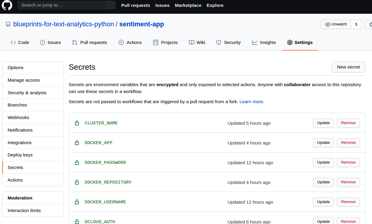
Figure 13-5. Adding credentials to your repository using secrets.
For the deployment steps, we have to connect to our running GCP cluster and update the image that we use for the deployment. First, we have to add PROJECT_ID, LOCATION_NAME, CLUSTER_NAME, and GCLOUD_AUTH to the secrets to enable this action. We encode these as secrets to ensure that project details of our cloud deployments are not stored publicly. You can get the GCLOUD_AUTH by using the provided instructions and adding the values in the downloaded key as the secret for this field.
The next steps for deployment include setting up the gcloud utility on the build machine and using this to get the Kubernetes configuration file:
    # Setup gcloud CLI
    - uses: GoogleCloudPlatform/github-actions/setup-gcloud@master
      with:
        version: '290.0.1'
        service_account_key: ${{ secrets.GCLOUD_AUTH }}
        project_id: ${{ secrets.PROJECT_ID }}

    # Get the GKE credentials so we can deploy to the cluster
    - run: |-
        gcloud container clusters get-credentials ${{ secrets.CLUSTER_NAME }} \
                                           --zone ${{ secrets.LOCATION_ZONE }}
Finally, we update the Kubernetes deployment with the latest Docker image. This is where we use the TAG_NAME to identify the latest release that we pushed in the second step. Finally, we add an action to monitor the status of the rollout in our cluster:
    # Deploy the Docker image to the GKE cluster
    - name: Deploy
      run: |-
        kubectl set image --record deployment.apps/sentiment-app \
                  sentiment-app=textblueprints/sentiment-app:\
                  ${{ steps.source_details.outputs.TAG_NAME }}

    # Verify that deployment completed
    - name: Verify Deployment
      run: |-
        kubectl rollout status deployment.apps/sentiment-app
        kubectl get services -o wide
You can follow the various stages of the build pipeline using the Actions tab of your repository, as shown in Figure 13-6. At the end of the deployment pipeline, an updated version of the API should be available at the same URL and can also be tested by visiting the API documentation.
This technique works well when code and model files are small enough to be packaged into the Docker image. If we use deep learning models, this is often not the case, and creating large Docker containers is not recommended. In such cases, we still use Docker containers to package and deploy our API, but the model files reside on the host system and can be attached to the Kubernetes cluster. For cloud deployments, this makes use of a persistent storage like Google Persistent Disk. In such cases, we can perform model updates by performing a cluster update and changing the attached volume.
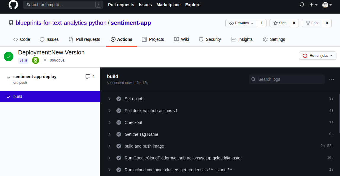
Figure 13-6. GitHub deployment workflow initiated by pushing a Git tag.
Closing Remarks
We introduced a number of blueprints with the aim of allowing you to share the analysis and projects you created using previous chapters in this book. We started by showing you how to create reproducible conda environments that will allow your teammate or a fellow learner to easily reproduce your results. With the help of Docker environments, we make it even easier to share your analysis by creating a complete environment that works regardless of the platform or infrastructure that your collaborators are using. If someone would like to integrate the results of your analysis in their product or service, we can encapsulate the machine learning model into a REST API that can be called from any language or platform. Finally, we provided a blueprint to easily create a cloud deployment of your API that can be scaled up or down based on usage. This cloud deployment can be updated easily with a new version of your model or additional functionality. While adding each layer of abstraction, we make the analysis accessible to a different (and broader) audience and reduce the amount of detail that is exposed.