Chapter 10. Exploring Semantic Relationships with Word Embeddings

The concept of similarity is fundamental to all machine learning tasks. In Chapter 5, we explained how to compute text similarity based on the bag-of-words model. Given two TF-IDF vectors for documents, their cosine similarity can be easily computed, and we can use this information to search, cluster, or classify similar documents.

However, the concept of similarity in the bag-of-words model is completely based on the number of common words in two documents. If documents do not share any tokens, the dot product of the document vectors and hence the cosine similarity will be zero. Consider the following two comments about a new movie, which could be found on a social platform:

“What a wonderful movie.”

“The film is great.”

Obviously, the comments have a similar meaning even though they use completely different words. In this chapter, we will introduce word embeddings as a means to capture the semantics of words and use them to explore semantic similarities within a corpus.

What You’ll Learn and What We’ll Build

For our use case we assume that we are market researchers and want to use texts about cars to better understand some relationships in the car market. Specifically, we want to explore similarities among car brands and models. For example, which models of brand A are most similar to a given model of brand B?

Our corpus consists of the 20 subreddits in the autos category of the Reddit Self-Posts dataset, which was already used in Chapter 4. Each of these subreddits contains 1,000 posts on cars and motorcycles with brands such as Mercedes, Toyota, Ford, and Harley-Davidson. Since those posts are questions, answers, and comments written by users, we will actually get an idea of what these users implicitly consider as being similar.

We will use the Gensim library again, which was introduced in Chapter 8. It provides a nice API to train different types of embeddings and to use those models for semantic reasoning.

After studying this chapter, you will be able to use word embeddings for semantic analysis. You will know how to use pretrained embeddings, how to train your own embeddings, how to compare different models, and how to visualize them. You can find the source code for this chapter along with some of the images in our GitHub repository.

The Case for Semantic Embeddings

In the previous chapters, we used the TF-IDF vectorization for our models. It is easy to compute, but it has some severe disadvantages:

• The document vectors have a very high dimensionality that is defined by the size of the vocabulary. Thus, the vectors are extremely sparse; i.e., most entries are zero.
• It does not work well for short texts like Twitter messages, service comments, and similar content because the probability for common words is low for short texts.
• Advanced applications such as sentiment analysis, question answering, or machine translation require capturing the real meaning of the words to work correctly.

Still, the bag-of-words model works surprisingly well for tasks such as classification or topic modeling, but only if the texts are sufficiently long and enough training data is available. Remember that similarity in the bag-of-words model is solely based on the existence of significant common words.

An embedding, in contrast, is a dense numerical vector representation of an object that captures some kind of semantic similarity. When we talk of embeddings in the context of text analysis, we have to distinguish word and document embeddings. A word embedding is a vector representation for a single word, while a document embedding is a vector representing a document. By document we mean any sequence of words, be it a short phrase, a sentence, a paragraph, or even a long article. In this chapter, we will focus on dense vector representations for words.

Word Embeddings

The target of an embedding algorithm can be defined as follows: given a dimensionality $d$, find vector representations for words such that words with similar meanings have similar vectors. The dimensionality $d$ is a hyperparameter of any word embedding algorithm. It is typically set to a value between 50 and 300.

The dimensions themselves have no predefined or human-understandable meaning. Instead, the model learns latent relations among the words from the text. Figure 10-1 (left) illustrates the concept. We have five-dimensional vectors for each word. Each of these dimensions represents some relation among the words so that words similar in that aspect have similar values in this dimension. Dimension names shown are possible interpretations of those values.

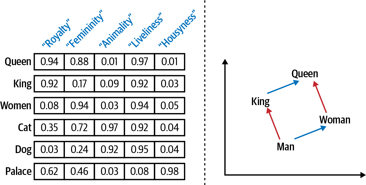
Figure 10-1. Dense vector representations captioning semantic similarity of words (left) can be used to answer analogy questions (right). We gave the vector dimensions hypothetical names like “Royalty” to show possible interpretations.¹

The basic idea for training is that words occurring in similar contexts have similar meanings. This is called the distributional hypothesis. Take, for example, the following sentences describing tesgüino:2

• A bottle of ___ is on the table.
• Everybody likes ___ .
• Don’t have ___ before you drive.
• We make ___ out of corn.

Even without knowing the word tesgüino, you get a pretty good understanding of its meaning by analyzing typical contexts. You could also identify semantically similar words because you know it’s an alcoholic beverage.

Analogy Reasoning with Word Embeddings

What’s really amazing is that word vectors built this way allow us to detect analogies like “queen is to king like woman is to man” with vector algebra (Figure 10-1, right). Let $v\left(w\right)$ be the word embedding for a word $w$. Then the analogy can be expressed mathematically like this:

$$v\left(queen\right)-v\left(king\right)\approx v\left(woman\right)-v\left(man\right)$$

If this approximate equation holds, we can reformulate the analogy as a question: What is to king like “woman” is to “man”? Or mathematically:³

$$v\left(woman\right)+\left[v\left(king\right)-v\left(man\right)\right]\approx ?$$

This allows some kind of fuzzy reasoning to answer analogy questions like this one: “Given that Paris is the capital of France, what is the capital of Germany?” Or in a market research scenario as the one we will explore: “Given that F-150 is a pickup truck from Ford, what is the similar model from Toyota?”

Types of Embeddings

Several algorithms have been developed to train word embeddings. Gensim allows you to train Word2Vec and FastText embeddings. GloVe embeddings can be used for similarity queries but not trained with Gensim. We introduce the basic ideas of these algorithms and briefly explain the more advanced but also more complex contextualized embedding methods. You will find the references to the original papers and further explanations at the end of this chapter.

Word2Vec

Even though there have been approaches for word embeddings before, the work of Tomáš Mikolov at Google (Mikolov et al., 2013) marks a milestone because it dramatically outperformed previous approaches, especially on analogy tasks such as the ones just explained. There exist two variants of Word2Vec, the continuous bag-of-words model (CBOW) and the skip-gram model (see Figure 10-2).

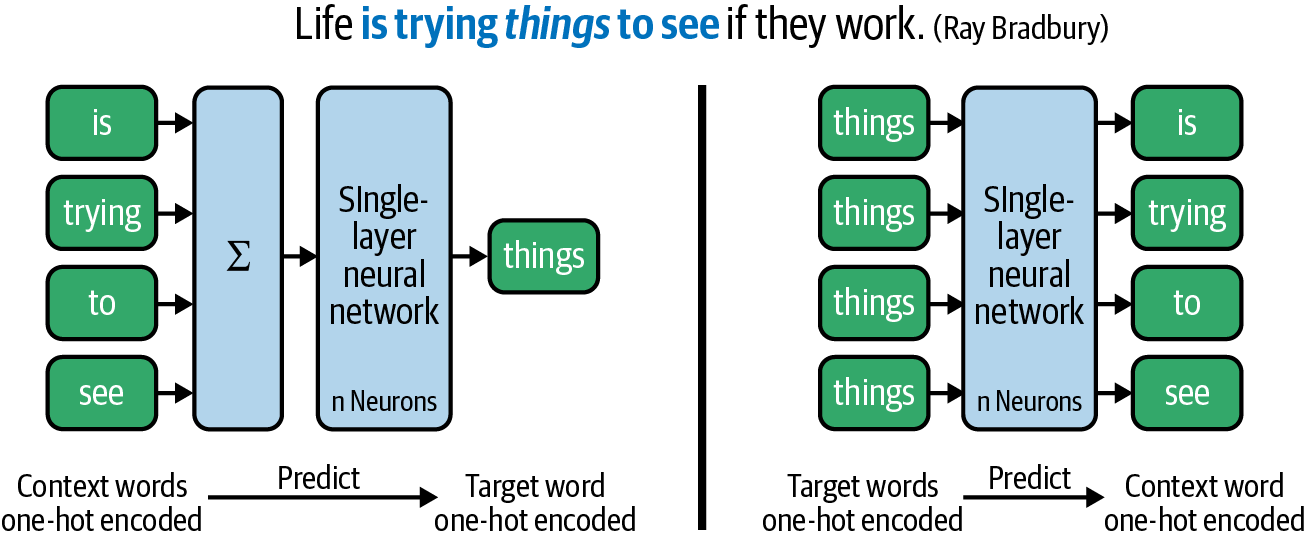
Figure 10-2. Continuous bag-of words (left) versus skip-gram model (right).

Both algorithms use a sliding window over the text, defined by a target word $w_t$ and the size of the context window $c$. In the example, $c=2$, i.e., the training samples consist of the five words $w_{t-2},\cdots ,w_{t+2}$. One such training sample is printed in bold: ... is trying things to see .... In the CBOW architecture (left), the model is trained to predict the target words from their context words. Here, a training sample consists of the sum or average of the one-hot encoded vectors of the context words and the target word as the label. In contrast, the skip-gram model (right) is trained to predict the context words given the target word. In this case, each target word generates a separate training sample for each context word; there is no vector averaging. Thus, skip-gram trains slower (much slower for large window sizes!) but often gives better results for infrequent words.

Both embedding algorithms use a simple single-layer neural network and some tricks for fast and scalable training. The learned embeddings are actually defined by the weight matrix of the hidden layer. Thus, if you want to learn 100-dimensional vector representations, the hidden layer has to consist of 100 neurons. The input and output words are represented by one-hot vectors. The dimensionality of the embeddings and size of the context window $c$ are hyperparameters in all of the embedding methods presented here. We will explore their impact on the embeddings later in this chapter.

GloVe

The GloVe (global vectors) approach, developed in 2014 by Stanford’s NLP group, uses a global co-occurrence matrix to compute word vectors instead of a prediction task (Pennington et al., 2014). A co-occurrence matrix for a vocabulary of size $V$ has the dimensionality $V\times V$. Each cell $(i,j)$ in the matrix contains the number of co-occurrences of the words $w_i$ and $w_j$ based again on a fixed context window size. The embeddings are derived using a matrix factorization technique similar to those used for topic modeling or dimensionality reduction.

The model is called global because the co-occurrence matrix captures global corpus statistics in contrast to Word2Vec, which uses only the local context window for its prediction task. GloVe does not generally perform better than Word2Vec but produces similarly good results with some differences depending on the training data and the task (see Levy et al., 2014, for a discussion).

FastText

The third model we introduce was developed again by a team with Tomáš Mikolov, this time at Facebook (Joulin et al., 2017). The main motivation was to handle out-of-vocabulary words. Both Word2Vec and GloVe produce word embeddings only for words contained in the training corpus. FastText, in contrast, uses subword information in the form of character n-grams to derive vector representations. The character trigrams for fasttext are, for example, fas, ast, stt, tte, tex, and ext. The lengths of n-grams used (minimum and maximum) are hyperparameters of the model.

Any word vector is built from the embeddings of its character n-grams. And that does work even for words previously unseen by the model because most of the character n-grams have embeddings. For example, the vector for fasttext will be similar to fast and text because of the common n-grams. Thus, FastText is pretty good at finding embeddings for misspelled words that are usually out-of-vocabulary.

Deep contextualized embeddings

The semantic meaning of a word often depends on its context. Think of different meanings of the word right in “I am right” and “Please turn right.”4 All three models (Word2Vec, GloVe, and FastText) have just one vector representation per word; they cannot distinguish between context-dependent semantics.

Contextualized embeddings like Embedding from Language Models (ELMo) take the context, i.e., the preceding and following words, into account (Peters et al., 2018). There is not one word vector stored for each word that can simply be looked up. Instead, ELMo passes the whole sentence through a multilayer bidirectional long short-term memory neural network (LSTM) and assembles the vectors for each word from weights of the internal layers. Recent models such as BERT and its successors improve the approach by using attention transformers instead of bidirectional LSTMs. The main benefit of all these models is transfer learning: the ability to use a pretrained language model and fine-tune it for specific downstream tasks such as classification or question answering. We will cover this concept in more detail in Chapter 11.

Blueprint: Using Similarity Queries on Pretrained Models

After all this theory, let’s start some practice. For our first examples, we use pretrained embeddings. These have the advantage that somebody else spent the training effort, usually on a large corpus like Wikipedia or news articles. In our blueprint, we will check out available models, load one of them, and do some reasoning with word vectors.

Loading a Pretrained Model

Several models are publicly available for download.5 We will describe later how to load custom models, but here we will use Gensim’s convenient downloader API instead.

Per the default, Gensim stores models under ~/gensim-data. If you want to change this to a custom path, you can set the environment variable GENSIM_DATA_DIR before importing the downloader API. We will store all models in the local directory models:

import os
os.environ['GENSIM_DATA_DIR'] = './models'

Now let’s take a look at the available models. The following lines transform the dictionary returned by api.info()['models'] into a DataFrame to get a nicely formatted list and show the first five of a total of 13 entries:

import gensim.downloader as api

info_df = pd.DataFrame.from_dict(api.info()['models'], orient='index')
info_df[['file_size', 'base_dataset', 'parameters']].head(5)

	file_size	base_dataset	parameters
fasttext-wiki-news-subwords-300	1005007116	Wikipedia 2017, UMBC webbase corpus and statmt.org news dataset (16B tokens)	{'dimension’: 300}
conceptnet-numberbatch-17-06-300	1225497562	ConceptNet, word2vec, GloVe, and OpenSubtitles 2016	{'dimension’: 300}
word2vec-ruscorpora-300	208427381	Russian National Corpus (about 250M words)	{'dimension’: 300, ‘window_size’: 10}
word2vec-google-news-300	1743563840	Google News (about 100 billion words)	{'dimension’: 300}
glove-wiki-gigaword-50	69182535	Wikipedia 2014 + Gigaword 5 (6B tokens, uncased)	{'dimension’: 50}

We will use the glove-wiki-gigaword-50 model. This model with 50-dimensional word vectors is small in size but still quite comprehensive and fully sufficient for our purposes. It was trained on roughly 6 billion lowercased tokens. api.load downloads the model if required and then loads it into memory:

model = api.load("glove-wiki-gigaword-50")

The file we downloaded actually does not contain a full GloVe model but just the plain word vectors. As the internal states of the model are not included, such reduced models cannot be trained further.

Similarity Queries

Given a model, the vector for a single word like king can be accessed simply via the property model.wv['king'] or even more simply by the shortcut model['king']. Let’s take a look at the first 10 components of the 50-dimensional vectors for king and queen.

v_king = model['king']
v_queen = model['queen']

print("Vector size:", model.vector_size)
print("v_king  =", v_king[:10])
print("v_queen =", v_queen[:10])
print("similarity:", model.similarity('king', 'queen'))

Out:

Vector size: 50
v_king  = [ 0.5   0.69 -0.6  -0.02  0.6  -0.13 -0.09  0.47 -0.62 -0.31]
v_queen = [ 0.38  1.82 -1.26 -0.1   0.36  0.6  -0.18  0.84 -0.06 -0.76]
similarity: 0.7839043

As expected, the values are similar in many dimensions, resulting in a high similarity score of over 0.78. So queen is quite similar to king, but is it the most similar word? Well, let’s check the three words most similar to king with a call to the respective function:

model.most_similar('king', topn=3)

Out:

[('prince', 0.824), ('queen', 0.784), ('ii', 0.775)]

In fact, the male prince is more similar than queen, but queen is second in the list, followed by the roman numeral II, because many kings have been named “the second.”

Similarity scores on word vectors are generally computed by cosine similarity, which was introduced in Chapter 5. Gensim provides several variants of similarity functions. For example, the cosine_similarities method computes the similarity between a word vector and an array of other word vectors. Let’s compare king to some more words:

v_lion = model['lion']
v_nano = model['nanotechnology']

model.cosine_similarities(v_king, [v_queen, v_lion, v_nano])

Out:

array([ 0.784,  0.478, -0.255], dtype=float32)

Based on the training data for the model (Wikipedia and Gigaword), the model assumes the word king to be similar to queen, still a little similar to lion, but not at all similar to nanotechnology. Note, that in contrast to nonnegative TF-IDF vectors, word embeddings can also be negative in some dimensions. Thus, the similarity values range from $+1$ to $-1$.

The function most_similar() used earlier allows also two parameters, positive and negative, each a list of vectors. If $positive=[po{s}_1,\cdots ,po{s}_n]$ and $negative=[ne{g}_1,\cdots ,ne{g}_m]$, then this function finds the word vectors most similar to ${\sum }_{i=1}^{n}po{s}_i-{\sum }_{j=1}^{m}ne{g}_j$.

Thus, we can formulate our analogy query about the royals in Gensim this way:

model.most_similar(positive=['woman', 'king'], negative=['man'], topn=3)

Out:

[('queen', 0.852), ('throne', 0.766), ('prince', 0.759)]

And the question for the German capital:

model.most_similar(positive=['paris', 'germany'], negative=['france'], topn=3)

Out:

[('berlin', 0.920), ('frankfurt', 0.820), ('vienna', 0.818)]

We can also leave out the negative list to find the word closest to the sum of france and capital:

model.most_similar(positive=['france', 'capital'], topn=1)

Out:

[('paris', 0.784)]

It is indeed paris! That’s really amazing and shows the great power of word vectors. However, as always in machine learning, the models are not perfect. They can learn only what’s in the data. Thus, by far not all similarity queries yield such staggering results, as the following example demonstrates:

model.most_similar(positive=['greece', 'capital'], topn=3)

Out:

[('central', 0.797), ('western', 0.757), ('region', 0.750)]

Obviously, there has not been enough training data for the model to derive the relation between Athens and Greece.

Note

Gensim also offers a variant of cosine similarity, most_similar_cosmul. This is supposed to work better for analogy queries than the one shown earlier because it smooths the effects of one large similarity term dominating the equation (Levy et al., 2015). For the previous examples, however, the returned words would be the same, but the similarity scores would be higher.

If you train embeddings with redacted texts from Wikipedia and news articles, your model will be able to capture factual relations like capital-country quite well. But what about the market research question comparing products of different brands? Usually you won’t find this information on Wikipedia but rather on up-to-date social platforms where people discuss products. If you train embeddings on user comments from a social platform, your model will learn word associations from user discussions. This way, it becomes a representation of what people think about a relationship, independent of whether this is objectively true. This is an interesting side effect you should be aware of. Often you want to capture exactly this application specific bias, and this is what we are going to do next. But be aware that every training corpus contains some bias, which may also lead to unwanted side effects (see “Man Is to Computer Programmer as Woman Is to Homemaker”).

Man Is to Computer Programmer as Woman Is to Homemaker

Most state-of-the-art approaches for NLP tasks ranging from classification to machine translation use semantic embeddings for better results. Thus, the quality of the embeddings has a direct impact on the quality of the final model. Unfortunately, machine learning algorithms have the tendency to amplify biases present in the training data. This is also true for word embeddings.

Bolukbasi et al., showed that “even word embeddings trained on Google News articles exhibit female/male gender stereotypes to a disturbing extent.” This is problematic, as a common approach is to use pretrained word embeddings for downstream tasks such as classification. Thus, debiasing training data is a hot topic in research nowadays.

Blueprints for Training and Evaluating Your Own Embeddings

In this section, we will train and evaluate domain-specific embeddings on 20,000 user posts on autos from the Reddit Selfposts dataset. Before we start training, we have to consider the options for data preparation as they always have a significant impact on the usefulness of a model for a specific task.

Data Preparation

Gensim requires sequences of tokens as input for the training. Besides tokenization there are some other aspects to consider for data preparation. Based on the distributional hypothesis, words frequently appearing together or in similar context will get similar vectors. Thus, we should make sure that co-occurrences are actually identified as such. If you do not have very many training sentences, as in our example here, you should include these steps in your preprocessing:

1. Clean text from unwanted tokens (symbols, tags, etc.).
2. Put all words into lowercase.
3. Use lemmas.

All this keeps the vocabulary small and training times short. Of course, inflected and uppercase words will be out-of-vocabulary if we prune our training data according to these rules. This is not a problem for semantic reasoning on nouns as we want to do, but it could be, if we wanted to analyze, for example, emotions. In addition, you should consider these token categories:

Stop words

Stop words can carry valuable information about the context of non-stop words. Thus, we prefer to keep the stop words.

Numbers

Depending on the application, numbers can be valuable or just noise. In our example, we are looking at auto data and definitely want to keep tokens like 328 because it’s a BMW model name. You should keep numbers if they carry relevant information.

Another question is whether we should split on sentences or just keep the posts as they are. Consider the imaginary post “I like the BMW 328. But the Mercedes C300 is also great.” Should these sentences be treated like two different posts for our similarity task? Probably not. Thus, we will treat the list of all lemmas in one user post as a single “sentence” for training.

We already prepared the lemmas for the 20,000 Reddit posts on autos in Chapter 4. Therefore, we can skip that part of data preparation here and just load the lemmas into a Pandas DataFrame:

db_name = "reddit-selfposts.db"
con = sqlite3.connect(db_name)
df = pd.read_sql("select subreddit, lemmas, text from posts_nlp", con)
con.close()

df['lemmas'] = df['lemmas'].str.lower().str.split() # lower case tokens
sents = df['lemmas'] # our training "sentences"

Phrases

Especially in English, the meaning of a word may change if the word is part of a compound phrase. Take, for example, timing belt, seat belt, or rust belt. All of these compounds have different meanings, even though all of them can be found in our corpus. So, it may better to treat such compounds as single tokens.

We can use any algorithm to detect such phrases, for example, spaCy’s detection of noun chunks (see “Linguistic Processing with spaCy”). A number of statistical algorithms also exist to identify such collocations, such as extraordinary frequent n-grams. The original Word2Vec paper (Mikolov et al., 2013) uses a simple but effective algorithm based on pointwise mutual information (PMI), which basically measures the statistical dependence between the occurrences of two words.

For the model that we are now training, we use an advanced version called normalized pointwise mutual information (NPMI) because it gives more robust results. And given its limited value range from $-1$ to $+1$, it is also easier to tune. The NPMI threshold in our initial run is set to a rather low value of 0.3. We choose a hyphen as a delimiter to connect the words in a phrase. This generates compound tokens like harley-davidson, which will be found in the text anyway. The default underscore delimiter would result in a different token:

from gensim.models.phrases import Phrases, npmi_scorer

phrases = Phrases(sents, min_count=10, threshold=0.3,
                  delimiter=b'-', scoring=npmi_scorer)

With this phrase model we can identify some interesting compound words:

sent = "I had to replace the timing belt in my mercedes c300".split()
phrased = phrases[sent]
print('|'.join(phrased))

Out:

I|had|to|replace|the|timing-belt|in|my|mercedes-c300

timing-belt is good, but we do not want to build compounds for combinations of brands and model names, like mercedes c300. Thus, we will analyze the phrase model to find a good threshold. Obviously, the chosen value was too low. The following code exports all phrases found in our corpus together with their scores and converts the result to a DataFrame for easy inspection:

phrase_df = pd.DataFrame(phrases.export_phrases(sents),
                         columns =['phrase', 'score'])
phrase_df = phrase_df[['phrase', 'score']].drop_duplicates() \
            .sort_values(by='score', ascending=False).reset_index(drop=True)
phrase_df['phrase'] = phrase_df['phrase'].map(lambda p: p.decode('utf-8'))

Now we can check what would be a good threshold for mercedes:

phrase_df[phrase_df['phrase'].str.contains('mercedes')]

	phrase	score
83	mercedes benz	0.80
1417	mercedes c300	0.47

As we can see, it should be larger than 0.5 and less than 0.8. Checking with a few other brands like bmw, ford, or harley davidson lets us identify 0.7 as a good threshold to identify compound vendor names but keep brands and models separate. In fact, with the rather stringent threshold of 0.7, the phrase model still keeps many relevant word combinations, for example, street glide (Harley-Davidson), land cruiser (Toyota), forester xt (Subaru), water pump, spark plug, or timing belt.

We rebuild our phraser and create a new column in our DataFrame with single tokens for compound words:

phrases = Phrases(sents, min_count=10, threshold=0.7,
                  delimiter=b'-', scoring=npmi_scorer)

df['phrased_lemmas'] = df['lemmas'].map(lambda s: phrases[s])
sents = df['phrased_lemmas']

The result of our data preparation steps are sentences consisting of lemmas and phrases. We will now train different embedding models and check which insights we can gain from them.

Blueprint: Training Models with Gensim

Word2Vec and FastText embeddings can be conveniently trained by Gensim. The following call to Word2Vec trains 100-dimensional Word2Vec embeddings on the corpus with a window size of 2, i.e., target word ±2 context words. Some other relevant hyperparameters are passed as well for illustration. We use the skip-gram algorithm and train the network in four threads for five epochs:

from gensim.models import Word2Vec

model = Word2Vec(sents,       # tokenized input sentences
                 size=100,    # size of word vectors (default 100)
                 window=2,    # context window size (default 5)
                 sg=1,        # use skip-gram (default 0 = CBOW)
                 negative=5,  # number of negative samples (default 5)
                 min_count=5, # ignore infrequent words (default 5)
                 workers=4,   # number of threads (default 3)
                 iter=5)      # number of epochs (default 5)

This takes about 30 seconds on an i7 laptop for the 20,000 sentences, so it is quite fast. More samples and more epochs, as well as longer vectors and larger context windows, will increase the training time. For example, training 100-dimensional vectors with a context window size of 30 requires about 5 minutes in this setting for skip-gram. The CBOW training time, in contrast, is rather independent of the context window size.

The following call saves the full model to disk. Full model means the complete neural network, including all internal states. This way, the model can be loaded again and trained further:

model.save('./models/autos_w2v_100_2_full.bin')

The choice of the algorithm as well as those hyperparameters have quite an impact on the resulting models. Therefore, we provide a blueprint to train and inspect different models. A parameter grid defines which algorithm variant (CBOW or skip-gram) and window sizes will be trained for Word2Vec or FastText. We could also vary vector size here, but that parameter does not have such a big impact. In our experience, 50- or 100-dimensional vectors work well on smaller corpora. So, we fix the vector size to 100 in our experiments:

from gensim.models import Word2Vec, FastText

model_path = './models'
model_prefix = 'autos'

param_grid = {'w2v': {'variant': ['cbow', 'sg'], 'window': [2, 5, 30]},
              'ft': {'variant': ['sg'], 'window': [5]}}
size = 100

for algo, params in param_grid.items():
    for variant in params['variant']:
        sg = 1 if variant == 'sg' else 0
        for window in params['window']:
            if algo == 'w2v':
                model = Word2Vec(sents, size=size, window=window, sg=sg)
            else:
                model = FastText(sents, size=size, window=window, sg=sg)

            file_name = f"{model_path}/{model_prefix}_{algo}_{variant}_{window}"
            model.wv.save_word2vec_format(file_name + '.bin', binary=True)

As we just want to analyze the similarities within our corpus, we do not save the complete models here but just the plain word vectors. These are represented by the class KeyedVectors and can be accessed by the model property model.wv. This generates much smaller files and is fully sufficient for our purpose.

Warning

Beware of information loss! When you reload models consisting only of the word vectors, they cannot be trained further. Moreover, FastText models lose the ability to derive embeddings for out-of-vocabulary words.

Blueprint: Evaluating Different Models

Actually, it is quite hard to algorithmically identify the best hyperparameters for a domain-specific task and corpus. Thus, it is not a bad idea to inspect the models manually and check how they perform to identify some already-known relationships.

The saved files containing only the word vectors are small (about 5 MB each), so we can load many of them into memory and run some comparisons. We use a subset of five models to illustrate our findings. The models are stored in a dictionary indexed by the model name. You could add any models you’d like to compare, even the pretrained GloVe model from earlier:

from gensim.models import KeyedVectors

names = ['autos_w2v_cbow_2', 'autos_w2v_sg_2',
         'autos_w2v_sg_5', 'autos_w2v_sg_30', 'autos_ft_sg_5']
models = {}

for name in names:
    file_name = f"{model_path}/{name}.bin"
    models[name] = KeyedVectors.load_word2vec_format(file_name, binary=True)

We provide a small blueprint function for the comparison. It takes a list of models and a word and produces a DataFrame with the most similar words according to each model:

def compare_models(models, **kwargs):

    df = pd.DataFrame()
    for name, model in models:
        df[name] = [f"{word} {score:.3f}"
                    for word, score in model.most_similar(**kwargs)]
    df.index = df.index + 1 # let row index start at 1
    return df

Now let’s see what effect the parameters have on our computed models. As we are going to analyze the car market, we check out the words most similar to bmw:

compare_models([(n, models[n]) for n in names], positive='bmw', topn=10)

	autos_w2v_cbow_2	autos_w2v_sg_2	autos_w2v_sg_5	autos_w2v_sg_30	autos_ft_sg_5
1	mercedes 0.873	mercedes 0.772	mercedes 0.808	xdrive 0.803	bmws 0.819
2	lexus 0.851	benz 0.710	335i 0.740	328i 0.797	bmwfs 0.789
3	vw 0.807	porsche 0.705	328i 0.736	f10 0.762	m135i 0.774
4	benz 0.806	lexus 0.704	benz 0.723	335i 0.760	335i 0.773
5	volvo 0.792	merc 0.695	x-drive 0.708	535i 0.755	mercedes_benz 0.765
6	harley 0.783	mercede 0.693	135i 0.703	bmws 0.745	mercedes 0.760
7	porsche 0.781	mercedes-benz 0.680	mercede 0.690	x-drive 0.740	35i 0.747
8	subaru 0.777	audi 0.675	e92 0.685	5-series 0.736	merc 0.747
9	mb 0.769	335i 0.670	mercedes-benz 0.680	550i 0.728	135i 0.746
10	volkswagen 0.768	135i 0.662	merc 0.679	435i 0.726	435i 0.744

Interestingly, the first models with the small window size of 2 produce mainly other car brands, while the model with window size 30 produces basically lists of different BMW models. In fact, shorter windows emphasize paradigmatic relations, i.e., words that can be substituted for each other in a sentence. In our case, this would be brands as we are searching for words similar to bmw. Larger windows capture more syntagmatic relations, where words are similar if they frequently show up in the same context. Window size 5, which is the default, produced a mix of both. For our data, paradigmatic relations are best represented by the CBOW model, while syntagmatic relations require a large window size and are therefore better captured by the skip-gram model. The outputs of the FastText model demonstrate its property that similarly spelled words get similar scores.

Looking for similar concepts

The CBOW vectors with window size 2 are pretty precise on paradigmatic relations. Starting from some known terms, we can use such a model to identify the central terms and concepts of a domain. Table 10-1 shows the output of some similarity queries on model autos_w2v_cbow_2. The column concept was added by us to highlight what kind of words we would expect as output.

Table 10-1. Most similar neighbors for selected words using the CBOW model with window size 2

Word	Concept	Most Similar
toyota	car brand	ford mercedes nissan certify dodge mb bmw lexus chevy honda
camry	car model	corolla f150 f-150 c63 is300 ranger 335i 535i 328i rx
spark-plug	car part	water-pump gasket thermostat timing-belt tensioner throttle-body serpentine-belt radiator intake-manifold fluid
washington	location	oregon southwest ga ottawa san_diego valley portland mall chamber county

Of course, the answers are not always correct with regard to our expectations; they are just similar words. For example, the list for toyota contains not only car brands but also several models. In real-life projects, however, domain experts from the business department can easily identify the wrong terms and still find interesting new associations. But manual curation is definitely necessary when you work with word embeddings this way.

Analogy reasoning on our own models

Now let’s find out how our different models are capable of detecting analogous concepts. We want to find out if Toyota has a product comparable to Ford’s F-150 pickup truck. So our question is: What is to “toyota” as “f150” is to “ford”? We use our function compare_models from earlier and transpose the result to compare the results of wv.most_similar() for different models:

compare_models([(n, models[n]) for n in names],
               positive=['f150', 'toyota'], negative=['ford'], topn=5).T

Out:

	1	2	3	4	5
autos_w2v_cbow_2	f-150 0.850	328i 0.824	s80 0.820	93 0.819	4matic 0.817
autos_w2v_sg_2	f-150 0.744	f-250 0.727	dodge-ram 0.716	tacoma 0.713	ranger 0.708
autos_w2v_sg_5	tacoma 0.724	tundra 0.707	f-150 0.664	highlander 0.644	4wd 0.631
autos_w2v_sg_30	4runner 0.742	tacoma 0.739	4runners 0.707	4wd 0.678	tacomas 0.658
autos_ft_sg_5	toyotas 0.777	toyo 0.762	tacoma 0.748	tacomas 0.745	f150s 0.744

In reality, the Toyota Tacoma is a direct competitor to the F-150 as well as the Toyota Tundra. With that in mind, the skip-gram model with the window size 5 gives the best results.6 In fact, if you exchange toyota for gmc, you get the sierra, and if you ask for chevy, you get silverado as the most similar to this model. All of these are competing full-size pickup trucks. This also works quite well for other brands and models, but of course it works best for those models that are heavily discussed in the Reddit forum.

Blueprints for Visualizing Embeddings

If we explore our corpus on the basis of word embeddings, as we do in this chapter, we are not interested in the actual similarity scores because the whole concept is inherently fuzzy. What we want to understand are semantic relations based on the concepts of closeness and similarity. Therefore, visual representations can be extremely helpful for the exploration of word embeddings and their relations. In this section, we will first visualize embeddings by using different dimensionality reduction techniques. After that, we will show how to visually explore the semantic neighborhood of given keywords. As we will see, this type of data exploration can reveal quite interesting relationships between domain-specific terms.

Blueprint: Applying Dimensionality Reduction

High-dimensional vectors can be visualized by projecting the data into two or three dimensions. If the projection works well, it is possible to visually detect clusters of related terms and get a much deeper understanding of semantic concepts in the corpus. We will look for clusters of related words and explore the semantic neighborhood of certain keywords in the model with window size 30, which favors syntagmatic relations. Thus, we expect to see a “BMW” cluster with BMW terms, a “Toyota” cluster with Toyota terms, and so on.

Dimensionality reduction also has many use cases in the area of machine learning. Some learning algorithms have problems with high-dimensional and often sparse data. Dimensionality reduction techniques such as PCA, t-SNE, or UMAP (see “Dimensionality Reduction Techniques”) try to preserve or even highlight important aspects of the data distribution by the projection. The general idea is to project the data in a way that objects close to each other in high-dimensional space are close in the projection and, similarly, distant objects remain distant. In our examples, we will use the UMAP algorithm because it provides the best results for visualization. But as the umap library implements the scikit-learn estimator interface, you can easily replace the UMAP reducer with scikit-learn’s PCA or TSNE classes.

Dimensionality Reduction Techniques

There are many different algorithms for dimensionality reduction. Frequently used for visualization are PCA, t-SNE, and UMAP.

Principal Component Analysis (PCA) performs a linear projection of the data such that most of the variance in the data points is preserved. Mathematically, it is based on the eigenvectors of the largest eigenvalues of the covariance matrix (the principal components). PCA only takes the global data distribution into account. Independent of local structures, all data points are transformed in the same way. Except for the number of dimensions in the target space (n_components), PCA has no hyperparameters to tune.

Nonlinear algorithms such as t-SNE and UMAP try to balance local and global aspects in the mapping. Thus, different areas of the original space get projected differently dependent on the local data distribution. Both algorithms provide hyperparameters that need to be carefully selected to produce good results. For t-SNE this is the perplexity (roughly the effective number of nearest neighbors of each point). For UMAP you need to specify the size of the local neighborhood (n_neighbors) and in addition the minimum distance of points in the projection (min_dist). t-SNE, published in 2008, is very popular but has some severe limitations. It preserves the local structure much better than the global structure, it does not scale well, and it works practically only for two or three dimensions. UMAP, published in 2018, is faster and retains the global data structure much better.

The following code block contains the basic operations to project the embeddings into two-dimensional space with UMAP, as shown in Figure 10-3. After the selection of the embedding models and the words to plot (in this case we take the whole vocabulary), we instantiate the UMAP dimensionality reducer with target dimensionality n_components=2. Instead of the standard Euclidean distance metric, we use the cosine as usual. The embeddings are then projected to 2D by calling reducer.fit_transform(wv).

from umap import UMAP

model = models['autos_w2v_sg_30']
words = model.vocab
wv = [model[word] for word in words]

reducer = UMAP(n_components=2, metric='cosine', n_neighbors = 15, min_dist=0.1)
reduced_wv = reducer.fit_transform(wv)

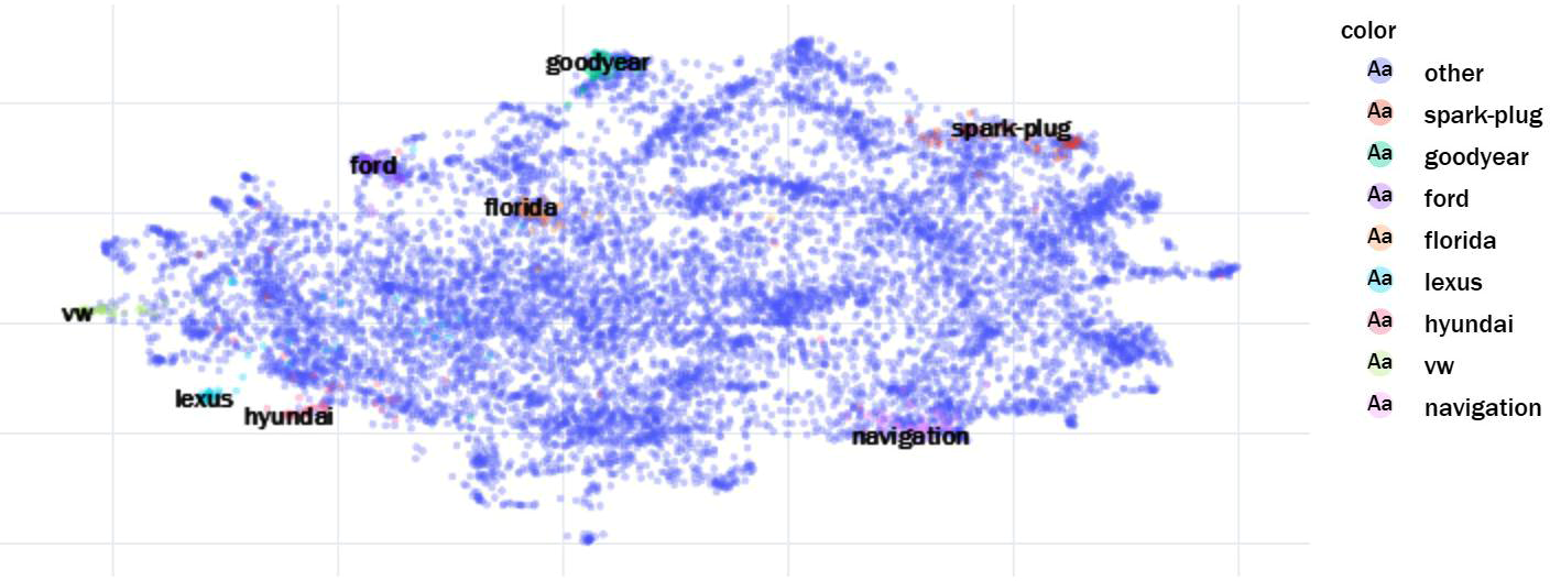
Figure 10-3. Two-dimensional UMAP projections of all word embeddings of our model. A few words and their most similar neighbors are highlighted to explain some of the clusters in this scatter plot.

We use Plotly Express here for visualization instead of Matplotlib because it has two nice features. First, it produces interactive plots. When you hover with the mouse over a point, the respective word will be displayed. Moreover, you can zoom in and out and select regions. The second nice feature of Plotly Express is its simplicity. All you need to prepare is a DataFrame with the coordinates and the metadata to be displayed. Then you just instantiate the chart, in this case the scatter plot (px.scatter):

import plotly.express as px

plot_df = pd.DataFrame.from_records(reduced_wv, columns=['x', 'y'])
plot_df['word'] = words
params = {'hover_data': {c: False for c in plot_df.columns},
          'hover_name': 'word'}

fig = px.scatter(plot_df, x="x", y="y", opacity=0.3, size_max=3, **params)
fig.show()

You can find a more general blueprint function plot_embeddings in the embeddings package in our GitHub repository. It allows you to choose the dimensionality reduction algorithm and highlight selected search words with their most similar neighbors in the low-dimensional projection. For the plot in Figure 10-3 we inspected some clusters manually beforehand and then explicitly named a few typical search words to colorize the clusters.⁷ In the interactive view, you could see the words when you hover over the points.

Here is the code to produce this diagram:

from blueprints.embeddings import plot_embeddings

search = ['ford', 'lexus', 'vw', 'hyundai',
          'goodyear', 'spark-plug', 'florida', 'navigation']

plot_embeddings(model, search, topn=50, show_all=True, labels=False,
                algo='umap', n_neighbors=15, min_dist=0.1)

For data exploration, it might be more interesting to visualize only the set of search words and their most similar neighbors, without all other points. Figure 10-4 shows an example generated by the following lines. Displayed are the search words and their top 10 most similar neighbors:

search = ['ford', 'bmw', 'toyota', 'tesla', 'audi', 'mercedes', 'hyundai']

plot_embeddings(model, search, topn=10, show_all=False, labels=True,
    algo='umap', n_neighbors=15, min_dist=10, spread=25)

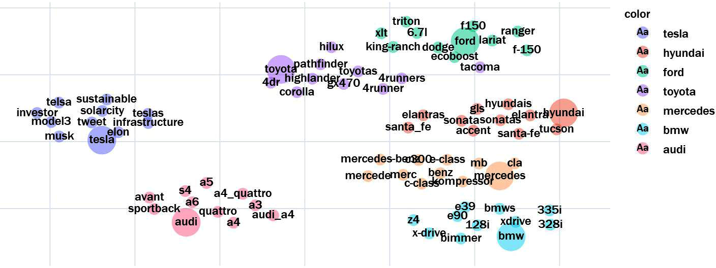
Figure 10-4. Two-dimensional UMAP projection of selected keywords words and their most similar neighbors.

Figure 10-5 shows the same keywords but with many more similar neighbors as a three-dimensional plot. It is nice that Plotly allows you to rotate and zoom into the point cloud. This way it is easy to investigate interesting areas. Here is the call to generate that diagram:

plot_embeddings(model, search, topn=30, n_dims=3,
    algo='umap', n_neighbors=15, min_dist=.1, spread=40)

To visualize analogies such as tacoma is to toyota like f150 is to ford, you should use the linear PCA transformation. Both UMAP and t-SNE distort the original space in a nonlinear manner. Therefore, the direction of difference vectors in the projected space can be totally unrelated to the original direction. Even PCA distorts because of shearing, but the effect is not as strong as in UMAP or t-SNE.

Figure 10-5. Three-dimensional UMAP projection of selected keywords and their most similar neighbors.

Blueprint: Using the TensorFlow Embedding Projector

A nice alternative to a self-implemented visualization function is the TensorFlow Embedding Projector. It also supports PCA, t-SNE, and UMAP and offers some convenient options for data filtering and highlighting. You don’t even have to install TensorFlow to use it because there is an online version available. A few datasets are already loaded as a demo.

To display our own word embeddings with the TensorFlow Embedding Projector, we need to create two files with tabulator-separated values: one file with the word vectors and an optional file with metadata for the embeddings, which in our case are simply the words. This can be achieved with a few lines of code:

import csv

name = 'autos_w2v_sg_30'
model = models[name]

with open(f'{model_path}/{name}_words.tsv', 'w', encoding='utf-8') as tsvfile:
    tsvfile.write('\n'.join(model.vocab))

with open(f'{model_path}/{name}_vecs.tsv', 'w', encoding='utf-8') as tsvfile:
    writer = csv.writer(tsvfile, delimiter='\t',
                        dialect=csv.unix_dialect, quoting=csv.QUOTE_MINIMAL)
    for w in model.vocab:
        _ = writer.writerow(model[w].tolist())

Now we can load our embeddings into the projector and navigate through the 3D visualization. For the detection of clusters, you should use UMAP or t-SNE. Figure 10-6 shows a cutout of the UMAP projection for our embeddings. In the projector, you can click any data point or search for a word and get the first 100 neighbors highlighted. We chose harley as a starting point to explore the terms related to Harley-Davidson. As you can see, this kind of visualization can be extremely helpful when exploring important terms of a domain and their semantic relationship.

Figure 10-6. Visualization of embeddings with TensorFlow Embedding Projector.

Blueprint: Constructing a Similarity Tree

The words with their similarity relations can be interpreted as a network graph in the following way: the words represent the nodes of the graph, and an edge is created whenever two nodes are “very” similar. The criterion for this could be either that the nodes are among their top-n most-similar neighbors or a threshold for the similarity score. However, most of the words in the vicinity of a word are similar not only to that word but also to each other. Thus, the complete network graph even for a small subset of words would have too many edges for comprehensible visualization. Therefore, we start with a slightly different approach and create a subgraph of this network, a similarity tree. Figure 10-7 shows such a similarity tree for the root word noise.

Figure 10-7. Similarity tree of words most similar to noise.

We provide two blueprint functions to create such visualizations. The first one, sim_tree, generates the similarity tree starting from a root word. The second one, plot_tree, creates the plot. We use Python’s graph library networkx in both functions.

Let’s first look at sim_tree. Starting from a root word, we look for the top-n most-similar neighbors. They are added to the graph with the according edges. Then we do the same for each of these newly discovered neighbors, and their neighbors, and so on, until a maximum distance to the root node is reached. Internally, we use a queue (collections.deque) to implement a breadth-first search. The edges are weighted by similarity, which is used later to style the line width:

import networkx as nx
from collections import deque

def sim_tree(model, word, top_n, max_dist):

    graph = nx.Graph()
    graph.add_node(word, dist=0)

    to_visit = deque([word])
    while len(to_visit) > 0:
        source = to_visit.popleft() # visit next node
        dist = graph.nodes[source]['dist']+1

        if dist <= max_dist: # discover new nodes
            for target, sim in model.most_similar(source, topn=top_n):
                if target not in graph:
                    to_visit.append(target)
                    graph.add_node(target, dist=dist)
                    graph.add_edge(source, target, sim=sim, dist=dist)
    return graph

The function plot_tree consists of just a few calls to create the layout and to draw the nodes and edges with some styling. We used Graphviz’s twopi layout to create the snowflake-like positioning of nodes. A few details have been left out here for the sake of simplicity, but you can find the full code on GitHub:

from networkx.drawing.nx_pydot import graphviz_layout

def plot_tree(graph, node_size=1000, font_size=12):

    pos = graphviz_layout(graph, prog='twopi', root=list(graph.nodes)[0])

    colors = [graph.nodes[n]['dist'] for n in graph] # colorize by distance
    nx.draw_networkx_nodes(graph, pos, node_size=node_size, node_color=colors,
                           cmap='Set1', alpha=0.4)
    nx.draw_networkx_labels(graph, pos, font_size=font_size)

    for (n1, n2, sim) in graph.edges(data='sim'):
         nx.draw_networkx_edges(graph, pos, [(n1, n2)], width=sim, alpha=0.2)

    plt.show()

Figure 10-7 was generated with these functions using this parametrization:

model = models['autos_w2v_sg_2']
graph = sim_tree(model, 'noise', top_n=10, max_dist=3)
plot_tree(graph, node_size=500, font_size=8)

It shows the most similar words to noise and their most similar words up to an imagined distance of 3 to noise. The visualization suggests that we created a kind of a taxonomy, but actually we didn’t. We just chose to include only a subset of the possible edges in our graph to highlight the relationships between a “parent” word and its most similar “child” words. The approach ignores possible edges among siblings or to grandparents. The visual presentation nevertheless helps to explore the specific vocabulary of an application domain around the root word. However, Gensim also implements Poincaré embeddings for learning hierarchical relationships among words.

The model with the small context window of 2 used for this figure brings out the different kinds and synonyms of noises. If we choose a large context window instead, we get more concepts related to the root word. Figure 10-8 was created with these parameters:

model = models['autos_w2v_sg_30']
graph = sim_tree(model, 'spark-plug', top_n=8, max_dist=2)
plot_tree(graph, node_size=500, font_size=8)

Figure 10-8. Similarity tree of words most similar to spark-plug’s most similar words.

Here, we chose spark-plug as root word and selected the model with window size 30. The generated diagram gives a nice overview about domain-specific terms related to spark-plugs. For example, the codes like p0302, etc., are the standardized OBD2 error codes for misfires in the different cylinders.

Of course, these charts also bring up some the weaknesses of our data preparation. We see four nodes for spark-plug, sparkplug, spark, and plugs, all of which are representing the same concept. If we wanted to have a single embedding for all of these, we would have to merge the different forms of writing into a single token.

Closing Remarks

Exploring the similar neighbors of certain key terms in domain-specific models can be a valuable technique to discover latent semantic relationships among words in a domain-specific corpus. Even though the whole concept of word similarity is inherently fuzzy, we produced really interesting and interpretable results by training a simple neural network on just 20,000 user posts about cars.

As in most machine learning tasks, the quality of the results is strongly influenced by data preparation. Depending on the task you are going to achieve, you should decide consciously which kind of normalization and pruning you apply to the original texts. In many cases, using lemmas and lowercase words produces good embeddings for similarity reasoning. Phrase detection can be helpful, not only to improve the result but also to identify possibly important compound terms in your application domain.

We used Gensim to train, store, and analyze our embeddings. Gensim is very popular, but you may also want to check possibly faster alternatives like (Py)Magnitude or finalfusion. Of course, you can also use TensorFlow and PyTorch to train different kinds of embeddings.

Today, semantic embeddings are fundamental for all complex machine learning tasks. However, for tasks such as sentiment analysis or paraphrase detection, you don’t need embeddings for words but for sentences or complete documents. Many different approaches have been published to create document embeddings (Wolf, 2018; Palachy, 2019). A common approach is to compute the average of the word vectors in a sentence. Some of spaCy’s models include word vectors in their vocabulary and allow the computation of document similarities based on average word vectors out of the box. However, averaging word vectors only works reasonably well for single sentences or very short documents. In addition, the whole approach is limited to the bag-of-words idea where the word order is not considered.

State-of-the-art models utilize both the power of semantic embeddings and the word order. We will use such a model in the next chapter for sentiment classification.

Further Reading

• Bolukbasi, Tolga, Kai-Wei Chang, James Zou, Venkatesh Saligrama, and Adam Kalai. Man Is to Computer Programmer as Woman Is to Homemaker? Debiasing Word Embeddings. 2016. https://arxiv.org/abs/1607.06520.

• Joulin, Armand, Edouard Grave, Piotr Bojanowski, and Tomáš Mikolov. Bag of Tricks for Efficient Text Classification. 2017. https://www.aclweb.org/anthology/E17-2068.

• Levy, Omer, Yoav Goldberg, and Ido Dagan. Improving Distributional Similarity with Lessons Learned from Word Embeddings. https://www.aclweb.org/anthology/Q15-1016.

• McCormick, Chris. Word2Vec Tutorial. http://mccormickml.com/2016/04/19/word2vec-tutorial-the-skip-gram-model and http://mccormickml.com/2017/01/11/word2vec-tutorial-part-2-negative-sampling.

• Mikolov, Tomáš, Kai Chen, Greg Corrado, and Jeffrey Dean. Efficient Estimation of Word Representations in Vector Space. 2013. https://arxiv.org/abs/1301.3781.

• Mikolov, Tomáš, Ilya Sutskever, Kai Chen, Greg Corrado, and Jeffrey Dean. Distributed Representations of Words and Phrases and Their Compositionality. 2013. https://arxiv.org/abs/1310.4546.

• Palachy, Shay. Beyond Word Embedding: Key Ideas in Document Embedding. https://www.kdnuggets.com/2019/10/beyond-word-embedding-document-embedding.html.

• Pennington, Jeffrey, Richard Socher, and Christopher Manning. Glove: Global Vectors for Word Representation. 2014. https://nlp.stanford.edu/pubs/glove.pdf.

• Peters, Matthew E., Mark Neumann, Mohit Iyyer, et al. Deep contextualized word representations. 2018. https://arxiv.org/abs/1802.05365.

• Wolf, Thomas. The Current Best of Universal Word Embeddings and Sentence Embeddings. 2018. https://medium.com/huggingface/universal-word-sentence-embeddings-ce48ddc8fc3a.

¹ Inspired by Adrian Colyer’s “The Amazing Power of Word Vectors” blog post.

² This frequently cited example originally came from the linguist Eugene Nida in 1975.

³ Jay Alammar’s blog post entitled “The Illustrated Word2Vec” gives a wonderful visual explanation of this equation.

⁴ Words having the same pronunciation but different meanings are called homonyms. If they are spelled identically, they are called homographs.

⁵ For example, from RaRe Technologies and 3Top.

⁶ If you run the code yourself, the results may be slightly different than the ones printed in the book because of random initialization.

⁷ You’ll find the colorized figures in the electronic versions and on GitHub.