Chapter 14. Search Engine
In Chapter 13 we discussed how to organize the knowledge we extract from text so that humans and expert systems can utilize it. Most people do not interact with data via graphs, though—especially text data. People generally want to search and retrieve the text. In Chapter 6, we introduced the basic concepts of information retrieval. We learned how to process text as well as how to calculate TF.IDF. In this chapter, we will build an actual search application.
The first thing we need to think about is what problem we are trying to solve. Rather than contrive a specific use case, let’s try and build an application that others can use to solve specific tasks. We want to build a tool that users can use to create a customized search.
We will need our application to do a few different things:
- Process text data
- Index the processed text
- Query the index
- Label search results to measure and improve the search experience
We used fictional scenarios in Chapters 12 and 13. Let’s see if we can make a tool that will actually be useful to us. We are the users here. This exercise will be useful because it is not uncommon that you will need to build tools for your own use.
Problem Statement and Constraints
What is the problem we are trying to solve?
We want to be able to build custom search engines that we can improve over time. We want this to be as reusable as possible. So we will want to build some abstractions into our application.
What constraints are there?
We will start with documents that have a title and text. Optionally, they can also contain other attributes—for example, categories, authors, and keywords. We want to be able to improve our search results without needing to re-index all the data. Also, we need to be able to label document-query pairs in order to improve our search engine.
How do we solve the problem with the constraints?
We need to consider multiple parts. First, we will process the text with Spark NLP and index it into Elasticsearch directly with Spark. We will build a special query that will utilize the fields of our documents. We will log the queries and the selection for each query.
Plan the Project
We will break this into chunks like in our previous project. This project will rely on organizing multiple open source technologies.
- Build processing and indexing script (Spark NLP, Elasticsearch)
- Customize query function
- Label document-query pairs (doccano)
For the first three steps, we will be using the Simple English Wikipedia data set. This is a good data set to use because it is not too large to work with on a personal machine, as the English Wikipedia would be. The benefit of using a wiki for this is that we will not require special knowledge to evaluate search results.
Design the Solution
In any real-world scenario, the code for the first two parts would need to be customized. What we can do is separate out the specialized code. This will allow us to reutilize the tools more easily in the future.
We will build an indexing script. First, this will parse and prepare the data for indexing. These are specialized steps that will need to be reimplemented for different data sources. The script will index the data. This is a more general piece of code. We will then build a query function that will allow the user to use different fields of the indexed documents in their query. Finally, we will look at labeling search results. The output of this can be used to improve the indexing script or to potentially implement a machine-learning–based ranker.
Implement the Solution
Before beginning the implementation, follow the appropriate instructions for installing Elasticsearch. You could also consider using the Elasticsearch Docker.
Once Elasticsearch is running, we can start to load and process the text.
import json
import re
import pandas as pd
import requests
import sparknlp

from pyspark.ml import Pipeline
from pyspark.sql import SparkSession, Row
from pyspark.sql.functions import lit, col

import sparknlp
from sparknlp import DocumentAssembler, Finisher
from sparknlp.annotator import *
packages = [
    'JohnSnowLabs:spark-nlp:2.2.2',
    'com.databricks:spark-xml_2.11:0.6.0',
    'org.elasticsearch:elasticsearch-spark-20_2.11:7.4.2'

]

spark = SparkSession.builder \
    .master("local[*]") \
    .appName("Indexing") \
    .config("spark.driver.memory", "12g") \
    .config("spark.jars.packages", ','.join(packages)) \
    .getOrCreate()
Loading and parsing the data will need to be specialized for different data sets. We should make sure that the output contains at least a text field, and a title field. You can include other fields that can be used to augment the search. For example, you could add the categories to the data. This allows for faceted searching, which is another way to say that you are filtering your results based on them having some property or facet.
# Loading the data - this will need to be specialized
df = spark.read\
    .format('xml')\
    .option("rootTag", "mediawiki")\
    .option("rowTag", "page")\
    .load("simplewiki-20191020-pages-articles-multistream.xml.bz2")\
    .repartition(200)\
    .persist()
# Selecting the data - this will need to be specialized
df = df.filter('redirect IS NULL').selectExpr(
    'revision.text._VALUE AS text',
    'title'
).filter('text IS NOT NULL')
# you must output a DataFrame that has a text field and a
# title field
Now that we have our data, let’s use Spark NLP to process it. This is similar to how we’ve processed data previously.
assembler = DocumentAssembler()\
    .setInputCol('text')\
    .setOutputCol('document')
tokenizer = Tokenizer()\
    .setInputCols(['document'])\
    .setOutputCol('tokens')
lemmatizer = LemmatizerModel.pretrained()\
    .setInputCols(['tokens'])\
    .setOutputCol('lemmas')
normalizer = Normalizer()\
    .setCleanupPatterns([
        '[^a-zA-Z.-]+',
        '^[^a-zA-Z]+',
        '[^a-zA-Z]+$',
    ])\
    .setInputCols(['lemmas'])\
    .setOutputCol('normalized')\
    .setLowercase(True)
finisher = Finisher()\
    .setInputCols(['normalized'])\
    .setOutputCols(['normalized'])

nlp_pipeline = Pipeline().setStages([
    assembler, tokenizer,
    lemmatizer, normalizer, finisher
]).fit(df)
processed = nlp_pipeline.transform(df)
Now, let’s select the fields we are interested in. We will be indexing the text, the title, and the normalized data. We want to store the actual text so that we can show it to the user. This may not always be the case, however. In federated search, you are combining data stored in different indices, and perhaps in other kinds of data stores, and searching it all at once. In federated search, you do not want to copy the data you will serve. Depending on how you are combining the search across data stores, you may need to copy some processed form of data. In this case, everything will be in Elasticsearch. We will search the title text and the normalized text. Think of these fields as helping with two different metrics. If a query matches a title, it is very likely a relevant document, but there are many queries for which the document is relevant that will not match with the title. Searching the normalized text will improve recall, but we still want title matches to affect the ranking more.
processed = processed.selectExpr(
    'text',
    'title',
    'array_join(normalized, " ") AS normalized'
)
Now we can index the DataFrame as is. We will pass the data directly to Elasticsearch. There are many options when creating an Elasticsearch index, so you should check out the API for Elasticsearch.
processed.write.format('org.elasticsearch.spark.sql')\
    .save('simpleenglish')
We can check what indices are available with the following cURL command.
! curl "http://localhost:9200/_cat/indices?v"
health status index         uuid                   pri rep docs.count docs.deleted store.size pri.store.size
yellow open   simpleenglish jVeJPRyATKKzPPEnuUp3ZQ   1   1     220858            0      1.6gb          1.6gb
It looks like everything is there. We can now query the index using the REST API. In order to query our index, we need to choose which fields we’ll query. Notice the fields that we list. The initial weights of the fields are guessed. As we learn how our users query the data, we can tune the weights.
headers = {
    'Content-Type': 'application/json',
}

params = (
    ('pretty', ''),
)

data = {
    "_source": ['title'],
    "query": {
        "multi_match": {
            "query": "data",
            "fields": ["normalized^1", "title^10"]
        },
    }
}

response = requests.post(
    'http://localhost:9200/simpleenglish/_search',
    headers=headers, params=params, data=json.dumps(data))

response.json()
{'took': 32,
 'timed_out': False,
 '_shards': {'total': 1, 'successful': 1, 'skipped': 0, 'failed': 0},
 'hits': {'total': {'value': 9774, 'relation': 'eq'},
  'max_score': 54.93799,
  'hits': [{'_index': 'simpleenglish',
    '_type': '_doc',
    '_id': '13iVYG4BfVJ3yetiTdZJ',
    '_score': 54.93799,
    '_source': {'title': 'Data'}},
   {'_index': 'simpleenglish',
    '_type': '_doc',
    '_id': '13iUYG4BfVJ3yeti720D',
    '_score': 45.704754,
    '_source': {'title': 'Repository (data)'}},
   ...
   {'_index': 'simpleenglish',
    '_type': '_doc',
    '_id': 'eHmWYG4BfVJ3yetiIs2m',
    '_score': 45.704754,
    '_source': {'title': 'Data collection'}}]}}
Now, let’s build our query function. The fields argument is expected to be a list of tuples of field names and boosts. Boosts are essentially weights that are applied to the scores returned from the index for different fields.
def query_index(query, fields=None, size=10):
    data = spark.createDataFrame([(text,)], ('text',))
    row = nlp_pipeline.transform(data).first()
    query = row['normalized'][0]

    if fields is None:
        fields = [('normalized', 1), ('title', 10)]

    headers = {
    'Content-Type': 'application/json',
    }
    params = (
        ('pretty', ''), ('size', size)
    )
    data = {
        "_source": ['title'],
        "query": {
            "multi_match": {
                "query": query,
                "fields": ['{}^{}'.format(f, b) for f, b in fields]
            },
        }
    }
    response = requests.post(
        'http://localhost:9200/simpleenglish/_search',
        headers=headers, params=params,
        data=json.dumps(data)).json()

    return [(r['_source']['title'], r['_score'])
            for r in response['hits']['hits']]
Now let’s build our set, which we will label. Let’s query the index for “Language.”
language_query_results = query_index('Language', size=13)
language_query_results
[('Language', 72.923416),
 ('Baure language', 60.667435),
 ('Luwian language', 60.667435),
 ('Faroese language', 60.667435),
 ('Aramaic language', 60.667435),
 ('Gun language', 60.667435),
 ('Beary language', 60.667435),
 ('Tigrinya language', 60.667435),
 ('Estonian language', 60.667435),
 ('Korean language', 60.667435),
 ('Kashmiri language', 60.667435),
 ('Okinawan language', 60.667435),
 ('Rohingya language', 60.667435)]
Returning articles about actual languages is a very reasonable result for the query “Language.”
We will need to make sure that we export the information necessary for our labeling, namely title and text. If your data has extra fields that you think will be relevant to judgments, you should modify the exported fields to include them. We will be creating documents for labeling. These documents will contain the query, the title, the score, and the text.
language_query_df = spark.createDataFrame(
    language_query_results, ['title', 'score'])

docs = df.join(language_query_df, ['title'])

docs = docs.collect()
docs = [r.asDict() for r in docs]

with open('lang_query_results.json', 'w') as out:
    for doc in docs:
        text = 'Query: Language\n'
        text += '=' * 50 + '\n'
        text += 'Title: {}'.format(doc['title']) + '\n'
        text += '=' * 50 + '\n'
        text += 'Score: {}'.format(doc['score']) + '\n'
        text += '=' * 50 + '\n'
        text += doc['text']
        line = json.dumps({'text': text})
        out.write(line + '\n')
Now that we have created the data we will need to label, let’s start using doccano. Doccano is a tool built to help in NLP labeling. It allows for document classification labeling (for tasks like sentiment analysis), segment labeling (for tasks like NER), and sequence-to-sequence labeling (for tasks like machine translation). You can set up this service locally or launch it in a docker. Let’s look at launching it in a docker.
First, we will pull the image.
docker pull chakkiworks/doccano
Next, we will run a container.
docker run -d --rm --name doccano \
  -e "ADMIN_USERNAME=admin" \
  -e "ADMIN_EMAIL=admin@example.com" \
  -e "ADMIN_PASSWORD=password" \
  -p 8000:8000 chakkiworks/doccano
If you plan on using doccano to have other people label, you should consider changing the admin credentials.
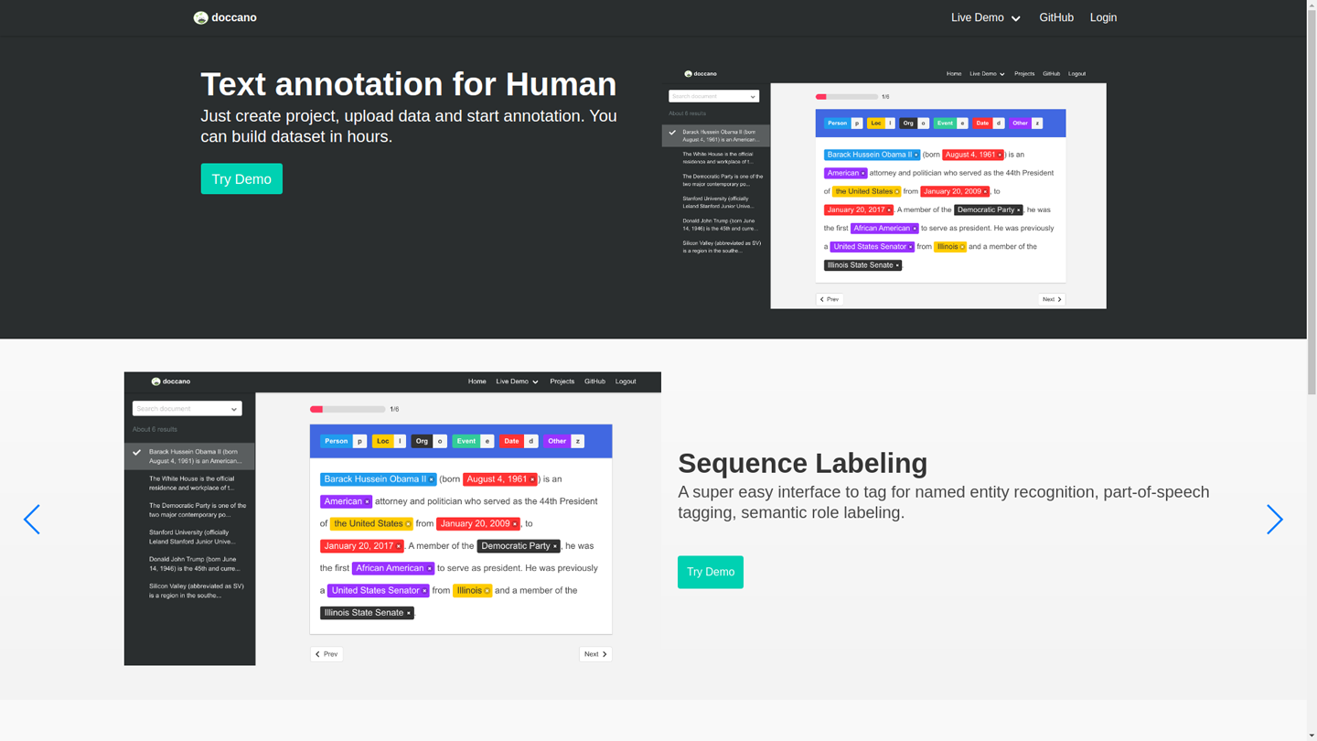
Once you have started the container, go to localhost:8000 (or whichever port you chose if you modified the -p argument). You should see the page in Figure 14-1.

Figure 14-1. Doccano landing page
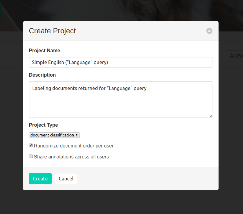
Click on the login and use the credentials from the docker run command. Then click “Create Project.” Here, in Figure 14-2, the project fields are filled out.

Figure 14-2. Creating a project in doccano
Next, click on “Select a file”, and navigate to the location lang_query_results.json created previously. This will add the documents for labeling to the project.
After this, click on “Labels,” and click “New label.” I added three, “relevant,” “partially relevant,” and “not relevant.” In the underlying data, these labels will be represented by the order in which you created them. For example, if you created “relevant,” “partially relevant,” and “not relevant” their representation will be 1, 2, 3, respectively.
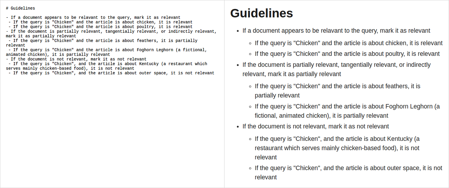
I think it is a good idea to write guidelines for labeling tasks, even if you are the one doing the labeling. This will help you think about how you want your data labeled. Figuring it out as you go can lead to inconsistencies.
Figure 14-3 is an example of the guidelines I created for this example task.

Figure 14-3. Guidelines in doccano
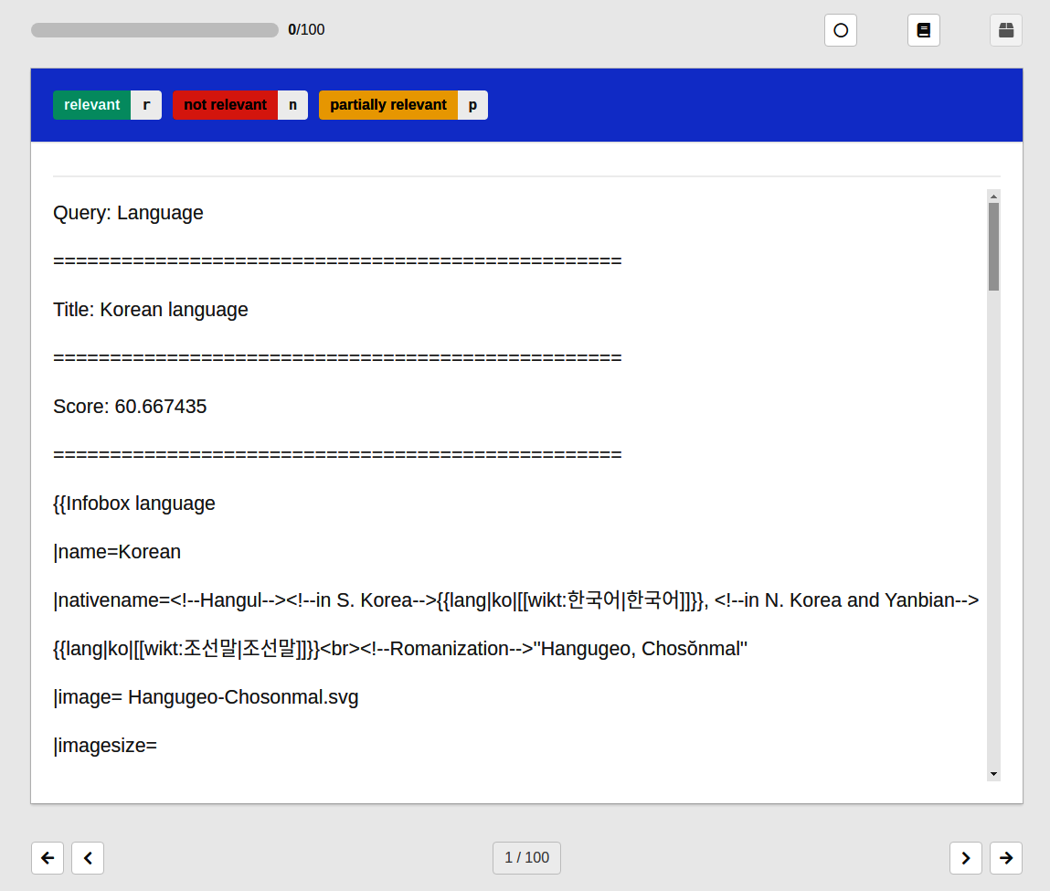
Now we are ready to begin labeling. Click on “Annotate Data,” and begin labeling. Figure 14-4 is a screenshot of the labeling page.

Figure 14-4. Doccano labeling
Once you are finished, you can click on “Edit Data,” which will take you back to the project page. From here, you can export the data by clicking “Export Data.” You can export as JSON lines or as CSV. We won’t be using this data, however, because labeling enough query-document pairs to improve the ranking would take some time.
Test and Measure the Solution
Now that we have created an index and have looked at how we can use doccano to label, we can talk about how we can measure our solution. This is a different scenario than most applications, since this tool will be used for organizing and retrieving documents for us—we are the customers.
Model-Centric Metrics
When measuring an index, there are many possible metrics. Primarily, we want the best ranking. One way to measure ranking is through recall and precision, which is similar to binary classification problems. The problem is that if we return a hundred documents, recall and precision will not tell us about the order they are in. For that, we need ranking metrics. One of the most popular kinds of metrics is Normalized Discounted Cumulative Gain (NDCG). To explain this, we need to build to it. First, let’s define gain. In this context, the gain is the information in the text. We use the relevancy of the document as gain. Cumulative gain is the sum of the gain up to a chosen cutoff. Up until this point there is nothing about rank, so we discount the gain the more we descend the list. We will need to reduce the gain using the rank. We use the logarithm of the rank so that the discount more strongly separates the items early in the list than those later in the list. The last part is the normalization. It is much easier to report a metric if it is between 0 and 1. So we need to determine the ideal discounted cumulative gain. If you cannot calculate it directly, you can estimate it assuming that all documents above the cutoff are relevant. Now let’s look at the actual metric.
Now, we can quantify how well our index works. Even if you are building a tool for yourself, it is important to quantify the quality of data-driven applications. Humans are the ultimate source of truth, but we are also fickle and moody. Using metrics can help make our evaluations dependable.
Review
When you are working on your own, reviewing is more difficult. If you have someone who is willing to help you review the work, they can provide a vital outside perspective. You want to value the time of your volunteer, so you should prepare a demo. More in-depth reviews are a more onerous request, so you can’t depend on being able to get a code review from a volunteer.
So how can we check for quality without assistance? We must put more effort into testing and documentation. This creates another problem—the increased effort in pursuit of quality can cause you to lose steam. This means that you should use such projects as an opportunity to set reasonable goals and milestones.
Conclusion
Information retrieval is a rich field of study. This chapter can serve as a starting point for you to delve into that field. The other important thing emphasized in this chapter is the value of projects built for yourself. In data science, it is often hard to find a professional opportunity to learn a new technique. Building a project for your own purpose can be a great opportunity to expand your collection of skills.
In Chapter 15, we will learn about building a model that works interactively with the user.